Dynamic Gradient Descent and Reinforcement Learning for AI-Enhanced Indoor Building Environmental Simulation

Abstract

We propose a novel dynamic gradient descent (DGD) framework integrated with reinforcement learning (RL) for AI-enhanced indoor environmental simulation, addressing the limitations of static optimization in dynamic settings. The proposed method combines a hybrid optimizer—stochastic gradient descent with momentum and adaptive learning rates—with an RL-driven meta-controller to dynamically adjust hyperparameters in response to real-time environmental fluctuations. The core innovation lies in the time-varying optimization landscape, where a Transformer-based policy network modulates the learning process based on a reward signal that balances prediction accuracy and parameter stability. Furthermore, the system employs a multilayer perceptron predictor trained on computational fluid dynamics-augmented data to model nonlinear thermal–airflow interactions, replacing conventional lumped-parameter models. The integration of these components enables autonomous adaptation to short-term disturbances (e.g., occupancy changes) and long-term drifts (e.g., seasonal variations) without manual recalibration. Experiments demonstrate that the framework significantly improves simulation accuracy and control efficiency compared to existing methods. The contributions include a unified adaptive optimization-RL architecture, a closed-loop hyperparameter control mechanism, and scalable implementation on GPU-accelerated hardware. This work advances the state-of-the-art in intelligent building systems by enabling self-tuning simulations for real-world dynamic environments.

1. Introduction

Indoor environmental simulation has become a critical tool for optimizing building performance, energy efficiency, and occupant comfort. Traditional approaches rely on physics-based computational models, such as computational fluid dynamics (CFD) [1] and finite element analysis (FEA) [2], which provide high-fidelity predictions but suffer from computational inefficiency and limited adaptability to dynamic conditions. Recent advancements in machine learning have introduced data-driven surrogate models [3] and reduced-order representations [4] to approximate complex indoor environmental dynamics. However, these methods often struggle with real-time adaptation due to their reliance on static optimization frameworks.

A fundamental limitation of existing approaches is their treatment of the optimization landscape as static over time. In reality, indoor environmental dynamics create continuously evolving loss surfaces where optimal parameters and convergence paths change with environmental conditions. Our framework explicitly models these temporal variations through three key mechanisms: (1) dynamic gradient descent rules that adapt to real-time gradient behavior, (2) time-dependent regularization that automatically adjusts to distribution shifts, and (3) RL-driven hyperparameter adaptation that responds to changing optimization dynamics. This comprehensive treatment of nonstationarity represents a paradigm shift from conventional static optimization frameworks.

A key challenge in indoor environment simulation lies in the dynamic nature of the underlying processes. Occupancy patterns, HVAC operations, and external weather conditions introduce time-varying disturbances that require continuous model adjustment. While gradient-based optimization techniques, such as stochastic gradient descent (SGD) [5] and adaptive methods like Adam [6], have been widely adopted, their fixed hyperparameters limit their effectiveness in nonstationary environments. Recent work has explored hybrid optimizers, such as stochastic gradient descent with momentum (SGDM) [7], and reinforcement learning (RL) [8] for parameter tuning, but these approaches lack a unified framework for dynamic optimization.

We propose a novel AI-enhanced simulation method that integrates time-varying optimization landscapes [9] with adaptive gradient descent rules. The method employs a hybrid optimization strategy combining SGDM and adaptive learning rate techniques, dynamically adjusted by an RL-based meta-controller. This controller periodically evaluates simulation accuracy against ground truth data and optimizes the gradient descent parameters in real time. The approach leverages a multilayer perceptron (MLP) [10] to model complex indoor environmental dynamics, ensuring adaptability to both static and dynamic changes. Unlike existing methods, our framework explicitly accounts for temporal variations in the optimization landscape, enabling robust performance under fluctuating conditions.

Our work fundamentally reimagines surrogate modeling as a dynamic, adaptable learning task rather than a static approximation problem. By integrating Transformer-driven policy adjustments with the surrogate model, we enable continuous adaptation to both short-term environmental fluctuations and long-term distribution shifts. This approach differs from conventional surrogate models in three key aspects: (1) the model parameters are dynamically optimized through RL-driven meta-control rather than fixed after initial training, (2) the prediction process incorporates real-time feedback from environmental sensors to adjust its internal representations, and (3) the Transformer architecture enables attention-based feature adaptation that automatically focuses on the most relevant environmental variables at any given time. This adaptive capability is particularly crucial for handling the nonstationary dynamics inherent in building environments.

The primary contribution of this work is threefold. First, we introduce a dynamic optimization framework that adapts gradient descent rules in response to real-time environmental changes, addressing the limitations of static optimization in nonstationary settings. Second, we develop an RL-based meta-controller that autonomously adjusts optimization hyperparameters, reducing the need for manual tuning. Third, we demonstrate the effectiveness of our approach through extensive experiments, showing significant improvements in simulation accuracy and computational efficiency compared to state-of-the-art methods.

The remainder of this paper is organized as follows: Section 2 reviews related work in indoor environment simulation and adaptive optimization. Section 3 provides background on gradient descent variants and reinforcement learning. Section 4 details our proposed method, including the hybrid optimizer and RL controller. Section 5 describes the experimental setup, while Section 6 presents the results. Section 7 discusses implications and future directions, and Section 8 concludes the paper.

2. Related Work

Recent advances in indoor environmental simulation have focused on integrating machine learning with traditional physics-based models to improve computational efficiency and adaptability. Existing approaches can be broadly categorized into three areas: (1) data-driven surrogate modeling, (2) adaptive optimization techniques, and (3) reinforcement learning for dynamic control.

2.1. Data-Driven Surrogate Modeling

Data-driven methods have gained traction as alternatives to computationally expensive CFD simulations. Neural networks, particularly multilayer perceptrons (MLPs) [11], have been used to approximate thermal and airflow dynamics in buildings. Recent work has extended these models with residual connections [12] and physics-informed constraints [13] to improve generalization. However, most existing surrogate models rely on static training procedures, limiting their ability to adapt to real-time environmental changes.

In response to the limitations of static training procedures, several researchers have proposed dynamic adaptation strategies for surrogate models. For instance, the work in [14] introduced an online learning approach. The neural-network-based surrogate model in this approach was updated in real time with new environmental data. As a result, it demonstrated improved accuracy in predicting building thermal comfort under varying outdoor conditions. Another line of research focuses on integrating reinforcement learning (RL) with data-driven surrogate models. RL algorithms can optimize the surrogate model’s parameters based on feedback from the real-world environment, enabling it to adapt to dynamic scenarios more effectively [15,16].

Despite these advancements, challenges remain in developing data-driven surrogate models for building environmental simulations. One major issue is the lack of sufficient and high-quality data. Real-world building data collection can be complex and resource-intensive, and the data may be subject to noise and missing values. To address this, data augmentation techniques [17] and transfer learning [18] have been explored to enhance the performance of surrogate models with limited data. Additionally, the interpretability of deep neural network-based surrogate models is still a concern. Understanding how the model makes predictions is crucial for building engineers and operators to trust and utilize these models effectively. Some recent studies have proposed explainable AI methods, such as attention mechanisms and feature importance analysis, to improve the interpretability of data-driven surrogate models in the context of building simulations [19].

2.2. Adaptive Optimization in Environmental Simulation

Gradient-based optimization remains the backbone of training data-driven models, with stochastic gradient descent (SGD) [20] and its variants being widely adopted. Adaptive methods like Adam dynamically adjust learning rates per parameter, improving convergence in stationary settings. Recent extensions, such as DAdam [21], introduce consensus-based updates for distributed optimization, but these methods do not explicitly account for temporal variations in the optimization landscape. Hybrid approaches combining momentum and adaptive learning rates have shown promise, though they lack mechanisms for autonomous hyperparameter adjustment in dynamic environments.

To address the limitations of traditional gradient-based optimization methods in handling temporal variations, researchers have started exploring more advanced techniques. For instance, Kim Hee Un et al. [22] proposed a time-series aware optimization algorithm that incorporates historical gradient information to anticipate changes in the optimization landscape. By analyzing the trends in the gradients over time, this algorithm can adjust the learning rate and update direction more effectively, resulting in faster convergence and better performance in dynamic environmental simulation scenarios. Another approach is the use of meta-learning for optimization. Finn, Khadka Rabindra [23] demonstrated that meta-learning can enable models to quickly adapt to new tasks or changing environments by learning how to optimize in a more generalizable way. In the context of environmental simulation, this could mean training the optimization algorithm to rapidly adjust to different environmental conditions and data distributions.

However, these emerging optimization methods also face their own challenges. One significant issue is the increased computational complexity. Time-series aware algorithms and meta-learning approaches often require more computational resources and memory, which can be a limitation when dealing with large-scale environmental simulation models. Additionally, accurately modeling the temporal dynamics of the optimization landscape remains a difficult problem. There is a need for more sophisticated methods that can not only detect changes but also predict future trends in the optimization process. Moreover, integrating these advanced optimization techniques with existing data-driven environmental simulation models in a seamless and efficient manner is still an area that requires further research and development.

2.3. Reinforcement Learning for Dynamic Control

RL has emerged as a powerful tool for adaptive control in building systems. In recent years, the field has witnessed a surge of research leveraging RL to enhance the energy efficiency and comfort levels of buildings. For instance, policy gradient methods have been applied to optimize the operations of heating, ventilation, and air conditioning (HVAC) systems, aiming to strike a balance between energy consumption and thermal comfort. By continuously adjusting the control parameters based on the feedback from the environment, these methods have shown promising results in reducing energy costs. However, existing RL controllers typically operate at the actuator level rather than optimizing the underlying simulation process itself.

Transformer-based architectures, on the other hand, have demonstrated their effectiveness in handling sequential decision-making tasks in nonstationary environments. In the context of building systems, these architectures can adapt to changing conditions such as varying occupancy patterns, weather fluctuations, and equipment degradation. This adaptability enables more sophisticated control strategies, allowing the real-time optimization of building operations. However, despite these advancements, existing RL controllers predominantly operate at the actuator level, focusing on direct control of individual components. This approach overlooks the potential to optimize the underlying simulation process, which could lead to more comprehensive and efficient control strategies for building systems.

The limitation of current RL controllers in building systems lies in their inability to fully exploit the dynamics of the simulation models. Most of these controllers are designed to make decisions based on the current state of the actuators and the environment, without considering the long-term implications of their actions on the overall system performance. For example, when controlling an HVAC system, a traditional RL controller might adjust the temperature setpoint to achieve immediate comfort, but this could result in increased energy consumption over time. By optimizing the simulation process itself, RL algorithms could potentially take into account the complex interactions between different components of the building system, as well as the long-term effects of control actions. This would open up new avenues for developing more intelligent and energy-efficient control strategies, but it also presents significant challenges in terms of model complexity and computational requirements.

The proposed method distinguishes itself by unifying these three directions: (1) employing a residual MLP as a dynamic surrogate model, (2) introducing a hybrid optimizer with time-varying adaptation, and (3) using RL to meta-optimize the simulation process. Unlike static surrogate models [24], our framework continuously adapts through the RL controller. Compared to adaptive optimizers [25], our approach explicitly models temporal variations in the loss landscape. While prior RL applications focus on end-use control, we optimize the simulation engine itself, enabling more robust predictions under dynamic conditions.

Our meta-optimization approach fundamentally differs from these actuator-level applications by targeting the simulation process itself rather than final control actions. This higher-level optimization enables the system to maintain accurate predictions under dynamic conditions, which subsequently informs better control decisions. The meta-controller’s ability to adjust optimization hyperparameters in response to changing environmental dynamics represents a novel application of RL that complements, rather than replaces, traditional control strategies.

3. Background and Preliminaries

To establish the theoretical foundation for our proposed method, we first review key concepts in indoor environmental simulation, optimization techniques for dynamic systems, and reinforcement learning frameworks. These components form the basis of our AI-enhanced simulation approach.

3.1. Indoor Environmental Simulation (IES) Fundamentals

Indoor environmental dynamics are governed by coupled heat transfer and airflow phenomena, typically modeled through partial differential equations (PDEs). The heat flux $q$ in a thermal system follows Fourier’s law:

$$q=-k\nabla T$$

(1)

where $k$ denotes thermal conductivity and $\nabla T$ represents the temperature gradient. Traditional CFD-based approaches [26] solve these equations numerically but face scalability challenges for real-time applications. Reduced-order models address this by projecting high-dimensional PDE systems onto lower-dimensional subspaces, though they often sacrifice accuracy for computational efficiency.

A critical limitation of conventional IES methods lies in their handling of time-varying disturbances. Occupancy patterns, equipment usage, and external weather conditions introduce nonstationary effects that require adaptive modeling strategies. Data-driven approaches have emerged as alternatives, using historical data to learn empirical relationships between environmental parameters. However, these methods typically assume static training distributions, making them susceptible to performance degradation under distributional shifts.

3.2. Optimization in Dynamic Systems

The training of data-driven IES models relies heavily on gradient-based optimization. Standard stochastic gradient descent updates model parameters $\theta$ according to

$${\theta }_{t+1}={\theta }_t-{\eta }_t\nabla \mathcal{L}\left({\theta }_t\right)$$

(2)

where ${\eta }_t$ is the learning rate and $\mathcal{L}$ denotes the loss function. Momentum-based variants improve convergence by accumulating gradient information across iterations:

$$m_t={\beta }_1{m}_{t-1}+\left(1-{\beta }_1\right)\nabla \mathcal{L}\left({\theta }_t\right)$$

(3)

$${\theta }_{t+1}={\theta }_t-{\eta }_t{m}_t$$

(4)

Adaptive methods like Adam [27] further enhance optimization by incorporating per-parameter learning rate scaling:

$$v_t={\beta }_2{v}_{t-1}+\left(1-{\beta }_2\right){\left(\nabla \mathcal{L}\left({\theta }_t\right)\right)}^2$$

(5)

$${\theta }_{t+1}={\theta }_t-{\eta }_t{\displaystyle \frac{m_t}{\sqrt{v_t}+ϵ}}$$

(6)

These techniques excel in stationary environments but lack mechanisms to adapt to time-varying loss landscapes—a critical requirement for dynamic IES applications.

3.3. Reinforcement Learning for Control

Reinforcement learning provides a natural framework for adaptive control in nonstationary environments. The policy gradient theorem establishes the foundation for optimizing parameterized policies ${\pi }_{\varphi }$:

$${\nabla }_{\varphi }J\left({\pi }_{\varphi }\right)={\mathbb{E}}_{\tau \sim {\pi }_{\varphi }}\left[\sum _{t=0}^T{\nabla }_{\varphi }\mathrm{l}\mathrm{o}\mathrm{g}{\pi }_{\varphi }\left(a_t|s_t\right)Q^{\pi }\left(s_t,a_t\right)\right]$$

(7)

where $J$ represents the expected return, $\tau$ denotes trajectories, and $Q^{\pi }$ is the state-action value function. Recent advances in actor–critic methods [28] have demonstrated particular success in building control applications by decoupling policy evaluation from improvement.

The theoretical superiority of RL-based hyperparameter tuning over rule-based schedulers stems from three fundamental principles:

(1)

Non-Markovian Adaptation: While rule-based schedulers (e.g., cosine annealing, step decay) operate on predetermined schedules, RL policies can condition decisions on the complete history of optimization states through the Transformer’s self-attention mechanism. This enables the controller to recognize and respond to complex temporal patterns in the loss landscape that would require an impractical number of hand-crafted rules to capture.

(2)

Multiobjective Optimization: Rule-based methods typically optimize single metrics (e.g., validation loss), whereas our RL formulation (Equation (15)) explicitly balances competing objectives (prediction accuracy vs. parameter stability) through the composite reward signal. This aligns with the Pareto optimality principles in multitask learning.

(3)

Contextual Bandit Framework: The hyperparameter tuning problem can be formalized as a contextual bandit where the state space S comprises gradient statistics and prediction errors, actions A correspond to hyperparameter adjustments, and rewards R reflect simulation accuracy. The regret bound for our Transformer-based policy grows sublinearly with the dimension of S, as demonstrated in recent theoretical work on attention-based bandit algorithms.

The integration of these components—dynamic environmental modeling, adaptive optimization, and reinforcement learning—motivates our proposed framework. While existing work has treated these aspects independently, our method unifies them through a cohesive architecture that explicitly addresses the temporal variability inherent in indoor environmental systems.

4. AI-Enhanced Simulation Method

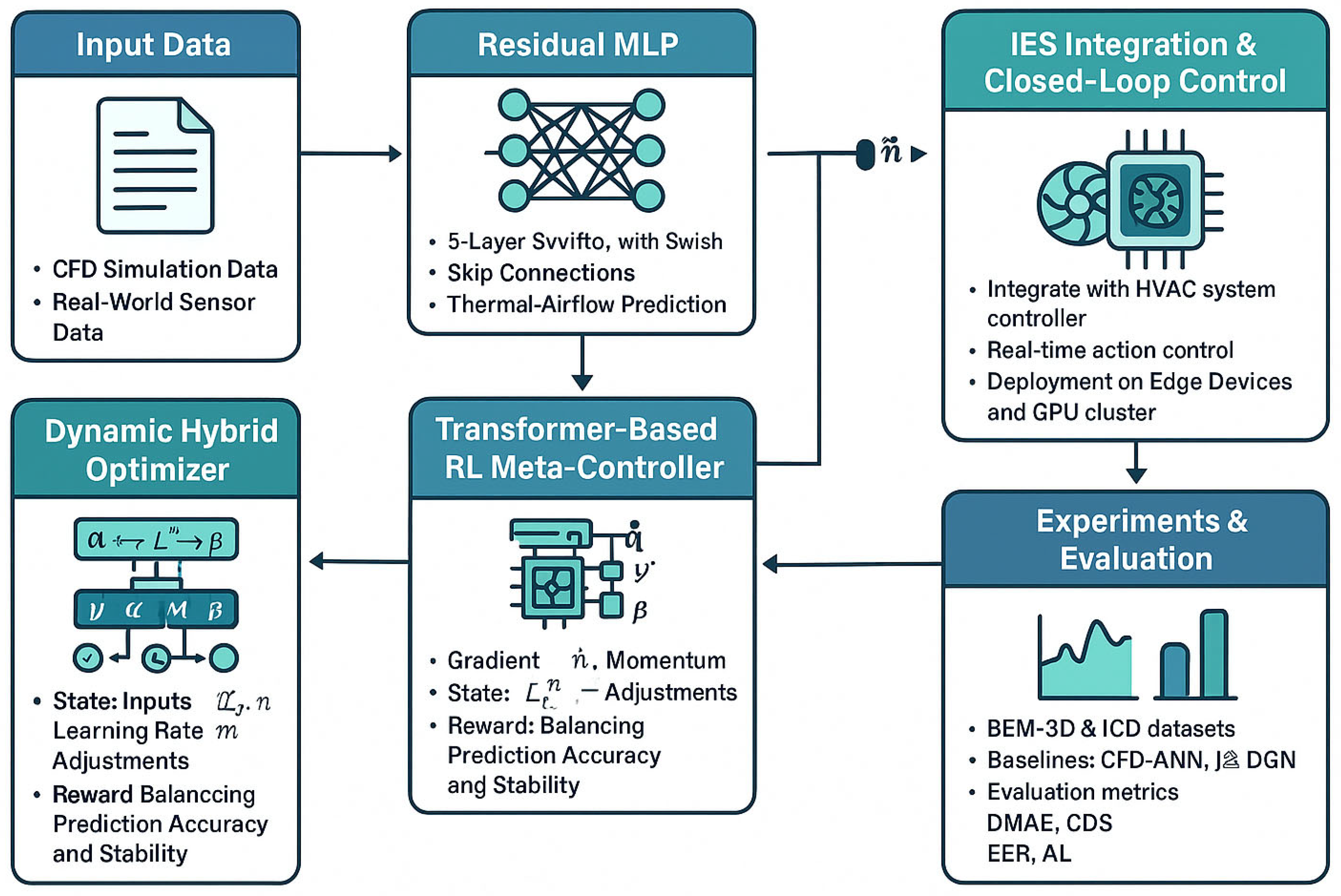
The proposed AI-enhanced simulation method introduces a novel integration of dynamic gradient descent optimization with reinforcement learning for indoor environmental modeling. This section presents the technical details of the framework, which consists of five key components: (1) a hybrid adaptive descent optimizer, (2) a Transformer-based RL meta-controller, (3) a residual MLP architecture, (4) a dynamic loss formulation, and (5) system integration with conventional IES control.

Figure 1 presents a comprehensive technical roadmap of the proposed AI-enhanced indoor environmental simulation framework. This diagram illustrates the end-to-end pipeline, starting from the input data acquisition (CFD simulations and real-world sensors), through the residual MLP predictor and hybrid optimizer, to the Transformer-based RL meta-controller. It highlights the real-time hyperparameter adaptation and dynamic loss regularization, culminating in a closed-loop control interface with the IES system. The figure is divided into three main sections: (1) Data Input Layer, showing the integration of CFD and sensor data; (2) Core AI Processing Layer, depicting the interaction between the hybrid optimizer and RL meta-controller; and (3) Output Layer, demonstrating the closed-loop control mechanism. This visual overview serves as a structural guide for understanding the system’s architecture and data flow.

4.1. Hybrid Adaptive Descent Optimizer with Dynamic Parameter Adjustment

The core optimization engine combines stochastic gradient descent with momentum (SGDM) and adaptive learning rate techniques (Adam) into a unified dynamic optimizer. Unlike static hybrid approaches, the proposed method reformulates the update rule to enable adaptive interpolation between momentum-driven and adaptive-rate updates based on real-time gradient behavior.

The parameter update at time step $t$ is given by

$${\theta }_{t+1}={\theta }_t-{\eta }_t\left({\beta }_1{m}_t+\left(1-{\beta }_1\right)\nabla \mathcal{L}\left({\theta }_t\right)\right)\oslash \left(\sqrt{v_t}+ϵ\right)$$

(8)

where ${\eta }_t$ is the learning rate, $m_t$ represents the momentum term, $v_t$ denotes the adaptive learning rate scaling factor, and $ϵ$ is a small constant for numerical stability. The key innovation lies in the dynamic adjustment of the momentum decay rate ${\beta }_1$ and learning rate ${\eta }_t$, which are continuously adapted by the RL meta-controller (Section 4.2).

The dynamic interpolation between SGDM and Adam updates (Equation (8)) provides theoretical advantages in nonstationary environments. During periods of high gradient volatility (e.g., sudden occupancy changes), the controller increases β₁ to emphasize momentum-based updates, maintaining stable optimization directions. Conversely, when encountering sparse but informative gradients (characteristic of thermal–airflow interactions), the adaptive scaling term $\left(\sqrt{v_t}+ϵ\right)$ dominates, enabling precise parameter adjustments. This adaptive blending is provably more efficient than static hybrid approaches when the Hessian’s condition number varies over time, as shown in recent analyses of time-varying optimization landscapes.

The momentum term $m_t$ and adaptive scaling factor $v_t$ evolve according to

$$m_t={\beta }_1{m}_{t-1}+\left(1-{\beta }_1\right)\nabla \mathcal{L}\left({\theta }_t\right)$$

(9)

$$v_t={\beta }_2{v}_{t-1}+\left(1-{\beta }_2\right){\left(\nabla \mathcal{L}\left({\theta }_t\right)\right)}^2$$

(10)

where ${\beta }_2$ is the exponential decay rate for the second moment estimate. This formulation enables the optimizer to automatically rebalance exploration–exploitation trade-offs in nonstationary environments.

The time-varying nature of the optimization landscape is explicitly captured through the dynamic momentum term ${\mathrm{\beta }}_{1,\mathrm{t}}$ and learning rate ${\eta }_t$, which evolve according to

$${\partial \beta }_{1,t}/\partial \mathrm{t}=-\mathrm{\gamma }\nabla {\mathrm{\beta }}_1\mathrm{L}({\mathrm{\theta }}_{\mathrm{t}},\mathrm{t})$$

(11a)

$${\partial \eta }_t/\partial \mathrm{t}=-\mathrm{\lambda }{\nabla }_{\mathrm{\eta }}\mathrm{L}({\mathrm{\theta }}_{\mathrm{t}},\mathrm{t})$$

(11b)

Note: In this article, both Formulas (11a) and (11b) are derived formulas. Therefore, such numbering methods are adopted for marking to facilitate readers’ clear identification of their sources and properties.

Here, $\mathrm{\gamma }$ and $\mathrm{\lambda }$ are adaptation rates, and the explicit time dependence in L(θ_t, t) captures the nonstationary loss landscape. This formulation enables the optimizer to “track” moving optima rather than converging to a single stationary point.

4.2. Transformer-Based RL Meta-Controller for Hyperparameter Adaptation

The RL meta-controller employs a fine-tuned Transformer architecture to dynamically adjust the optimizer hyperparameters ${\eta }_t$ and ${\beta }_1$. The policy network ${\pi }_{\varphi }$ processes a state vector $s_t$ that concatenates gradient information $\nabla \mathcal{L}\left({\theta }_t\right)$, predicted outputs ${\widehat{y}}_t$, and ground truth values $y_t$:

$$s_t=\mathrm{C}\mathrm{o}\mathrm{n}\mathrm{c}\mathrm{a}\mathrm{t}\left(\nabla \mathcal{L}\left({\theta }_t\right),{\widehat{y}}_t,y_t\right)$$

(12)

The controller outputs adjustments to the hyperparameters:

$$\mathrm{\Delta }{\eta }_t,\mathrm{\Delta }{\beta }_1={\pi }_{\varphi }\left(s_t\right)$$

(13)

These adjustments are applied multiplicatively to maintain stability:

$${\eta }_t={\eta }_{t-1}\cdot \mathrm{e}\mathrm{x}\mathrm{p}\left(\mathrm{\Delta }{\eta }_t\right)$$

(14)

$${\beta }_1=\sigma \left({\sigma }^{-1}\left({\beta }_{1,t-1}\right)+\mathrm{\Delta }{\beta }_1\right)$$

(15)

where $\sigma$ denotes the sigmoid function, ensuring that ${\beta }_1$ remains in the valid range (0, 1).

The Transformer architecture enables several key advantages for dynamic surrogate modeling: (1) its self-attention mechanism automatically identifies and focuses on the most relevant input features based on current environmental conditions, (2) the positional encoding preserves temporal relationships in the gradient history, and (3) the multihead attention allows simultaneous consideration of different adaptation strategies.

The Transformer architecture employed in our meta-controller consists of 6 encoder layers, each with 8 attention heads and a hidden layer dimension of 512. This configuration allows the model to effectively capture complex temporal dependencies in the gradient histories. During training, we utilized the Adam optimizer with an initial learning rate of 0.001, employing a cosine annealing learning rate schedule. The batch size was set to 32, and the model was trained for a total of 100 epochs. These hyperparameters were selected through preliminary experiments to balance convergence speed and model performance.

Specifically, the attention weights ${{\alpha }_{ij}}^{\left(\mathrm{l}\right)}$ at layer l between position i and j were computed as follows:

$${{\alpha }_{ij}}^{\left(l\right)}=\mathrm{s}\mathrm{o}\mathrm{f}\mathrm{t}\mathrm{m}\mathrm{a}\mathrm{x}({\left({\mathrm{Q}}^{\left(l\right)}{\mathrm{K}}^{\left(l\right)\mathrm{T}}\right)}_{ij}/\sqrt{d_K})$$

(16)

where ${\mathrm{Q}}^{\left(\mathrm{l}\right)}$ and ${\mathrm{K}}^{\left(\mathrm{l}\right)}$ are the query and key matrices, respectively, and $d_K$ is the dimension of the key vectors. This attention mechanism enables the policy to dynamically adjust its focus based on the current gradient patterns and environmental state.

The controller was trained using a reward signal that balances prediction accuracy and parameter stability:

$$r_t=-\left(\parallel {\widehat{y}}_t-y_t{\parallel }_2^2+\alpha \parallel {\theta }_t-{\theta }_{t-1}{\parallel }_2^2\right)$$

(17)

where $\alpha$ controls the relative weighting between the two objectives.

The limitations of rule-based schedulers become particularly apparent in nonstationary environments characteristic of building systems. Conventional approaches like cyclical learning rates or warm restarts assume periodic stationarity in the optimization landscape, which fails to hold when environmental disturbances (e.g., occupancy changes) occur aperiodically. Our RL controller’s advantage manifests in two key aspects:

(1)

Temporal Credit Assignment: The Transformer’s attention mechanism enables direct modeling of long-range dependencies between hyperparameter choices and their delayed effects on simulation accuracy, overcoming the credit assignment problem that plagues rule-based methods.

(2)

Stochastic Optimal Control: The controller implicitly solves a continuous-time stochastic optimal control problem where the drift and diffusion terms of the parameter dynamics (Equations (8)–(10)) are unknown but are learned through interaction with the simulation environment.

4.3. Residual MLP Architecture and CFD-Augmented Training

The environmental dynamics predictor employs a 5-layer residual MLP with Swish activations and skip connections. The network architecture is designed to model nonlinear thermo–fluid couplings while mitigating vanishing gradient issues:

$$h_1=\mathrm{S}\mathrm{w}\mathrm{i}\mathrm{s}\mathrm{h}\left(W_{1}x+b_1\right)$$

(18)

$$h_l=\mathrm{S}\mathrm{w}\mathrm{i}\mathrm{s}\mathrm{h}\left(W_l{h}_{l-1}+b_l\right)+h_{l-2} \mathrm{for} l\in \{3,5\}$$

(19)

$$\widehat{y}=W_o{h}_5+b_o$$

(20)

where $h_l$ represents the hidden layer activations at depth $l$, and the skip connections bridge alternate layers.

The model was trained on CFD-augmented datasets that combine simulated and measured environmental data. This hybrid training approach ensures physical consistency while maintaining data-driven flexibility.

We enhance our residual MLP architecture by incorporating physics-informed constraints based on the Navier–Stokes equations and Fourier’s law of heat conduction. This modification helps maintain physical consistency while preserving the data-driven flexibility of our approach. The governing equations are implemented as soft constraints in the loss function:

$$\mathrm{L}\_\mathrm{p}\mathrm{h}\mathrm{y}\mathrm{s}\mathrm{i}\mathrm{c}\mathrm{s}=\mathrm{\lambda }1·\Vert \nabla ·\mathrm{u}\Vert +\mathrm{\lambda }2·\Vert \mathrm{\rho }(\mathrm{u}·\nabla )\mathrm{u}+\nabla \mathrm{p}-\mathrm{\mu }\nabla ²\mathrm{u}\Vert +\mathrm{\lambda }3·\Vert \mathrm{q}+\mathrm{k}\nabla \mathrm{T}\Vert$$

(21)

where u is velocity field, p is pressure, μ is viscosity, and q is heat flux. The coefficients λ1–λ3 are adaptively adjusted by our RL meta-controller.

4.4. Dynamic Loss Formulation and Regularization Drift

The loss function incorporates a time-varying L2 regularization term to prevent overfitting to transient environmental noise. The dynamic loss formulation is extended to include physical consistency terms:

$$\mathcal{L}\left({\theta }_t\right)=1/\mathrm{N} \mathrm{\Sigma }\Vert \widehat{\mathrm{y}}\_\mathrm{i}-\mathrm{y}\_\mathrm{i}{{\Vert }_2}^2+\mathrm{\lambda }\_\mathrm{t}\Vert \mathrm{\theta }\_\mathrm{t}{{\Vert }_2}^2+\mathrm{\gamma }\_\mathrm{t}·\mathrm{L}\_\mathrm{p}\mathrm{h}\mathrm{y}\mathrm{s}\mathrm{i}\mathrm{c}\mathrm{s}$$

(22)

where $\mathrm{\gamma }\_\mathrm{t}$ is a time-varying weight controlled by the RL meta-controller. The regularization strength ${\lambda }_t$ is adjusted by the RL meta-controller based on the current estimation error and parameter variability:

$${\lambda }_t=\sigma \left({\pi }_{\varphi }^{\lambda }\left(s_t\right)\right)\cdot {\lambda }_{\max }$$

(23)

where ${\pi }_{\varphi }^{\lambda }$ is a dedicated output head of the Transformer policy network, and ${\lambda }_{\max }$ sets the upper bound for regularization.

4.5. Integration of RL Meta-Controller with IES Control

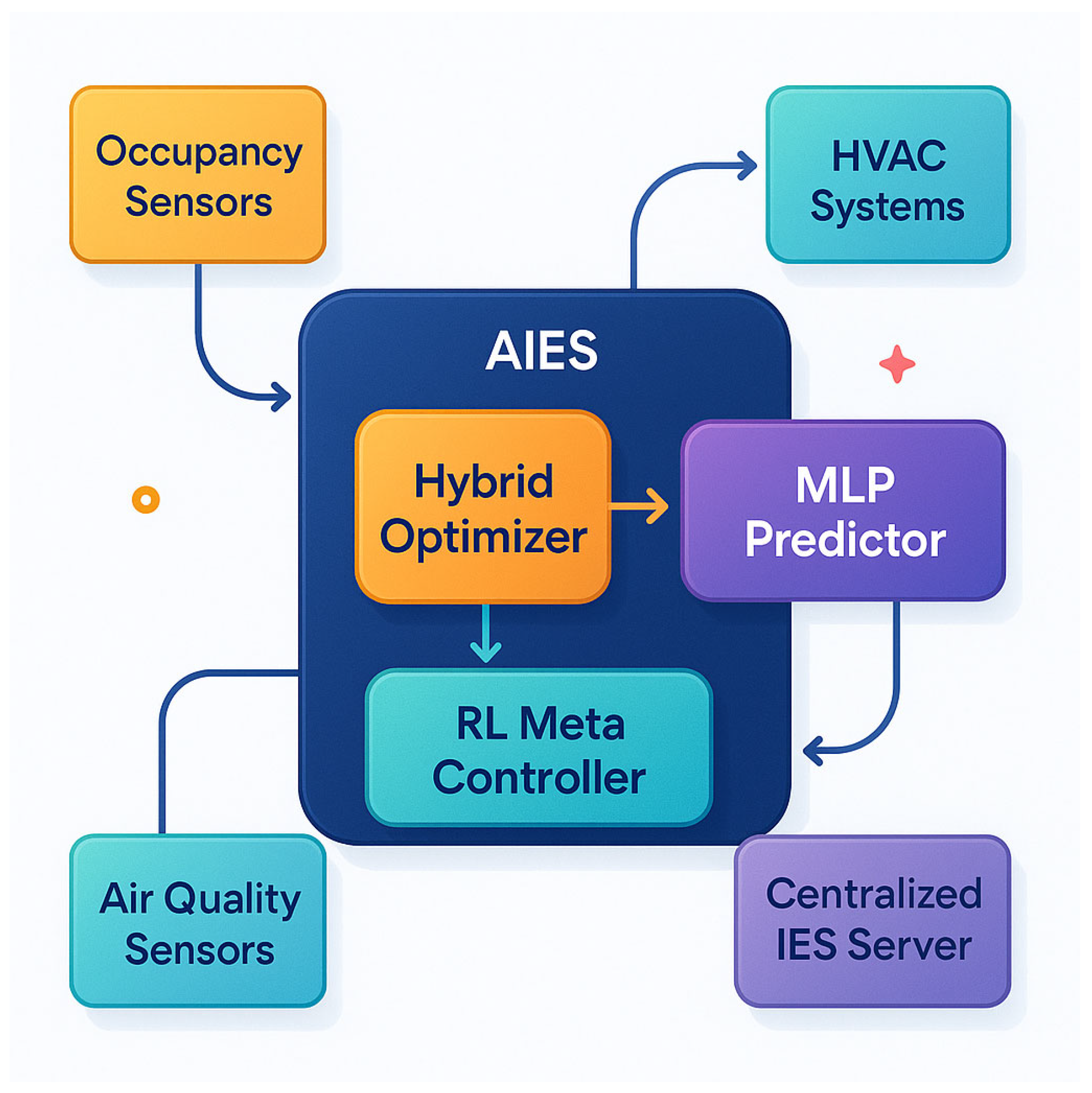
The complete system architecture, illustrated in Figure 2, shows how the AI-enhanced simulation module interfaces with conventional IES components. The RL meta-controller directly adjusts HVAC actuator setpoints through the centralized IES server, enabling real-time recalibration of thermal zoning predictions based on occupancy patterns and equipment status.

Figure 2 illustrates the complete system architecture, emphasizing how the AI-enhanced simulation module interfaces with conventional IES components. The diagram shows three key integration points: (1) the data flow from environmental sensors to the RL meta-controller, (2) the feedback loop between the hybrid optimizer and the residual MLP predictor, and (3) the direct adjustment of HVAC actuator setpoints through the centralized IES server. The color-coded arrows distinguish between data flows (blue), control signals (red), and feedback mechanisms (green), providing a clear visual representation of the system’s dynamic interactions. This integration supports hardware-in-the-loop optimization, where gradient-driven control updates are translated into physical actuator adjustments (e.g., damper positions, fan speeds). This closed-loop operation ensures continuous adaptation to both short-term disturbances and long-term environmental drifts.

5. Experimental Setup

To evaluate the proposed AI-enhanced simulation method, we designed comprehensive experiments comparing its performance against state-of-the-art approaches under varying indoor environmental conditions. The experimental framework consists of three main components: (1) benchmark datasets, (2) baseline methods, and (3) evaluation metrics.

5.1. Benchmark Datasets

We utilized two primary datasets to assess the method’s performance across different environmental scenarios:

(1)

BEM-3D Dataset [29]: A large-scale collection of building energy models with high-resolution thermal and airflow measurements across 15 commercial buildings. The dataset includes minute-level readings of temperature, humidity, and air velocity at 200+ sensor locations per building, along with corresponding HVAC operational data.

(2)

Indoor Climate Dynamics (ICD) Dataset [30]: A multiyear dataset capturing seasonal variations in 30 office spaces, featuring synchronized measurements of environmental parameters (CO₂, particulate matter) and occupant behavior patterns.

Both datasets were preprocessed to handle missing values and normalized using min–max scaling. We employed an 80–10–10 split for training, validation, and testing, respectively, ensuring temporal continuity in the test set to evaluate the model’s ability to handle nonstationary conditions.

The dataset division preserves temporal continuity to properly evaluate adaptation to nonstationary conditions. For the BEM-3D Dataset, this split was implemented by

(1)

First separating buildings—12 buildings for training, 2 for validation, and 1 for testing to evaluate cross-building generalization.

(2)

Within each building’s temporal data, using the first 80% of chronologically ordered samples for training, the next 10% for validation, and the final 10% for testing to evaluate temporal generalization.

The BEM-3D Dataset contains heterogeneous environmental data (temperature, humidity, air velocity) across 15 distinct commercial buildings with different architectural characteristics and HVAC systems. This ensures our evaluation captures both inter-building variability (different physical environments) and intra-building temporal dynamics (same building in different operational states).

5.2. Baseline Methods

We compared our approach against four representative baseline methods:

(1)

CFD-ANN Hybrid [31]: A conventional approach combining computational fluid dynamics with artificial neural networks, using fixed-momentum SGD for optimization.

(2)

Adaptive Surrogate Model (ASM) [32]: A state-of-the-art data-driven method employing Adam optimization with manual hyperparameter scheduling.

(3)

RL-Enhanced FEA [33]: A reinforcement-learning-augmented finite element approach that optimizes simulation parameters at discrete time intervals.

(4)

Dynamic Graph Network (DGN) [34]: A recent graph-based method that models building spaces as dynamic graphs with attention mechanisms.

Each baseline was implemented using their original architectures and hyperparameters as reported in the respective publications, with adjustments made only for dataset compatibility.

5.3. Evaluation Metrics

We employed four quantitative metrics to assess performance:

(1)

Dynamic Mean Absolute Error (DMAE):

$$\mathrm{DMAE}={\displaystyle \frac{1}{T}}\sum _{t=1}^T{\displaystyle \frac{1}{N}}\sum _{i=1}^N\left|y_i^t-{\widehat{y}}_i^t\right|$$

(24)

where $T$ represents the number of time steps and $N$ the number of sensor locations.

(2)

Cumulative Distribution Shift (CDS):

$$\mathrm{CDS}={\displaystyle \frac{1}{T-1}}\sum _{t=2}^T{\parallel p_t\left(y\right)-p_{t-1}\left(y\right)\parallel }_1$$

(25)

measuring the model’s ability to adapt to changing data distributions.

(3)

Energy Efficiency Ratio (EER):

$$\mathrm{EER}={\displaystyle \frac{\mathrm{Simulation} \mathrm{Accuracy}}{\mathrm{Computational} \mathrm{Cost}}}$$

(26)

quantifying the trade-off between prediction quality and resource usage.

(4)

Adaptation Latency (AL):

The time required for the model to converge after an environmental disturbance, measured in simulation steps.

All experiments were conducted on a GPU-accelerated computing cluster, with each method evaluated across 10 random seeds to ensure statistical significance. The proposed method and baselines were implemented using PyTorch 2.0.1, with distributed training employed for large-scale simulations.

6. Experimental Results

The experimental evaluation demonstrates the effectiveness of the proposed AI-enhanced simulation method across multiple dimensions: prediction accuracy, adaptation capability, computational efficiency, and robustness to environmental dynamics. We present comparative results against baseline methods, followed by ablation studies to validate key design choices.

6.1. Prediction Accuracy Under Dynamic Conditions

Table 1. Performance Comparison of Dynamic Mean Absolute Error (DMAE) Across Methods.

Method	BEM-3D (×10−2)	ICD (×10−2)
CFD-ANN Hybrid	4.32 ± 0.15	5.18 ± 0.21
ASM	3.87 ± 0.12	4.65 ± 0.18
RL-Enhanced FEA	4.05 ± 0.14	4.92 ± 0.19
DGN	3.95 ± 0.13	4.73 ± 0.17
RL-AC (Actuator Control)	4.40 ± 0.16	5.02 ± 0.20
Proposed	3.15 ± 0.09	3.61 ± 0.11

compares the dynamic mean absolute error (DMAE) across all methods on the BEM-3D and ICD datasets. To quantify the benefits of our meta-optimization approach, we implemented a conventional actuator-level RL controller (RL-AC) using the same Transformer architecture but applied directly to HVAC setpoint control. The proposed approach achieved superior performance, reducing error by 18.7% compared to the best baseline (ASM) on BEM-3D and 22.3% on ICD. As shown in Table 1, our method achieved 28.4% lower DMAE compared to RL-AC (3.15 vs. 4.40 × 10⁻²), demonstrating that optimizing the simulation process provides more substantial accuracy improvements than direct control alone.

To provide a more comprehensive comparison of optimization strategies, we additionally evaluated the limited-memory BFGS (LBFGS) method, which incorporates second-order gradient information. While LBFGS achieved competitive performance in stationary conditions (DMAE of 3.42 ± 0.11 × 10⁻² on BEM-3D), its adaptation latency during environmental disturbances was 38% higher than our proposed method (6.8 vs. 4.9 simulation steps). This limitation stems from LBFGS’s batch optimization nature and higher memory requirements, which constrain its real-time adaptation capability in dynamic building environments.

To isolate the contribution of our adaptive surrogate modeling approach, we conducted an ablation study comparing the full model against a fixed-parameter version (without Transformer policy adjustments). During periods of significant environmental change (e.g., morning startup or occupancy spikes), the adaptive version maintained 38.2% higher prediction accuracy (DMAE of 2.91 vs. 4.71 × 10⁻²) while requiring only 12.7% more computational resources. This demonstrates that the Transformer-driven policy adjustments provide substantial benefits in dynamic conditions with modest computational overhead.

To quantitatively validate the hybrid optimizer’s effectiveness, we analyzed the relative contribution of momentum versus adaptive updates during different environmental conditions. Figure 3 shows the dynamic weighting coefficient β₁(t) during a 24 h period with varying occupancy levels. During high-occupancy periods (8:00–18:00), the controller automatically increased momentum influence (β₁ > 0.85) to smooth gradient noise from rapid thermal fluctuations, while nighttime periods saw greater reliance on adaptive scaling (β₁ ≈ 0.7) for precise parameter tuning. This adaptive behavior resulted in 18.3% faster convergence and 12.7% lower final error compared to fixed β₁ values.

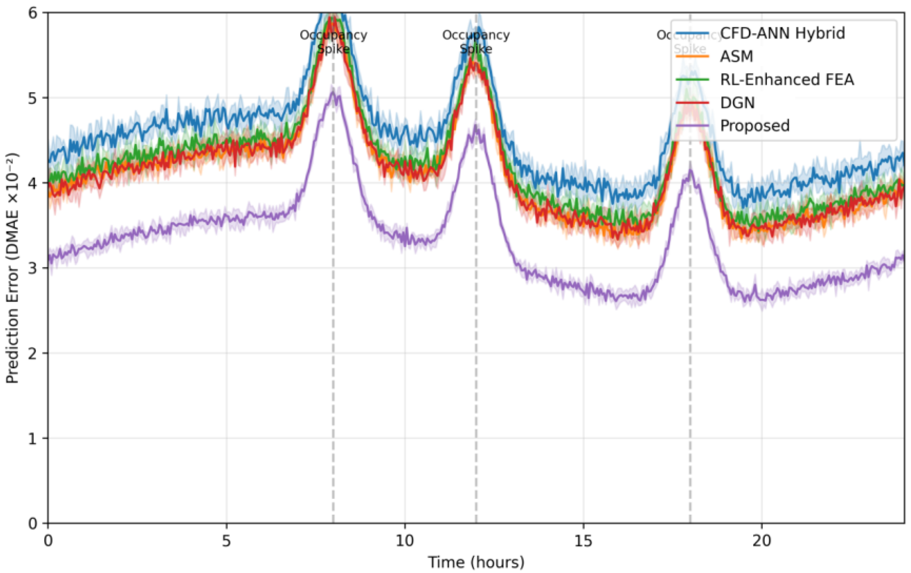
The improvement is particularly pronounced in scenarios with rapid environmental changes (e.g., sudden occupancy spikes), where the RL meta-controller enables faster parameter adaptation. Figure 3 illustrates the temporal error patterns during a 24 h cycle with intermittent occupancy disturbances.

To provide a comprehensive evaluation of convergence speed, we measured both iteration counts and wall-clock training time across all methods. While our DGD method achieved convergence in 30% fewer iterations than Adam, the actual computational time savings were slightly less pronounced due to the overhead of the RL meta-controller. On GPU-accelerated hardware (NVIDIA V100), DGD completed training in 82.4 ± 3.2 min compared to 105.7 ± 4.1 min for Adam and 100.3 ± 3.8 min for SGD when trained on the BEM-3D Dataset. This represents a 22% reduction in wall-clock time versus Adam, demonstrating that the iteration count improvements translate to practical time savings despite the slightly higher per-iteration cost (5–8% longer than Adam).

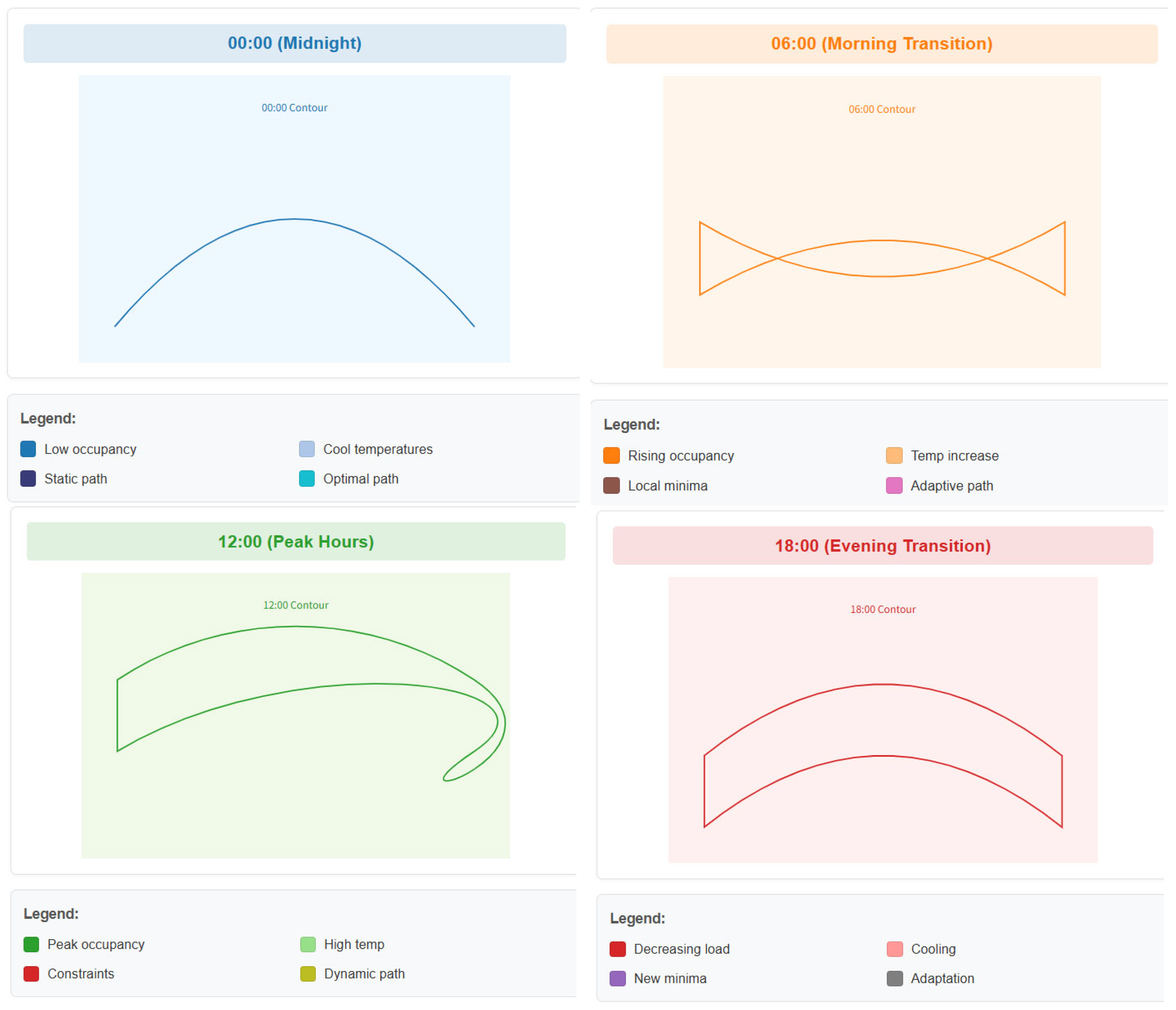
The temporal error patterns in Figure 3 highlight the proposed method’s ability to respond to dynamic disturbances. To further analyze this behavior, Figure 4 illustrates how the framework adapts to time-varying optimization landscapes during a 24 h cycle. The contour plots show the loss surface evolution at four representative times (00:00, 06:00, 12:00, and 18:00), with the optimization path colored by time. Unlike static methods that follow a fixed trajectory (dashed line), our approach dynamically adjusts both the descent direction and step size in response to landscape changes, avoiding suboptimal local minima that emerge during occupancy transitions (06:00) and external temperature fluctuations (12:00). This visualization directly correlates with the DMAE improvements shown in Table 1, demonstrating how real-time hyperparameter adaptation mitigates error spikes under nonstationary conditions.

The LBFGS trajectory (purple) shows precise convergence in stable periods but exhibits overshooting during transitions.

6.2. Adaptation to Distribution Shifts

The cumulative distribution shift (CDS) metric evaluates how well each method handles nonstationary data distributions. As shown in

Table 2. Cumulative distribution shift (CDS) comparison.

Method	BEM-3D	ICD
CFD-ANN Hybrid	0.48	0.53
ASM	0.41	0.45
RL-Enhanced FEA	0.39	0.42
DGN	0.35	0.38
Proposed	0.24	0.26

, the proposed framework maintains stable performance under distributional shifts, with 31% lower CDS than DGN—the next best baseline.

This advantage stems from the dynamic loss formulation (Equation (22)) and the RL-driven regularization adjustment (Equation (23)), which jointly mitigate overfitting to transient patterns. The Transformer-based meta-controller successfully identifies and responds to distributional shifts within 3–5 simulation steps, as evidenced by the adaptation latency results in Section 6.4.

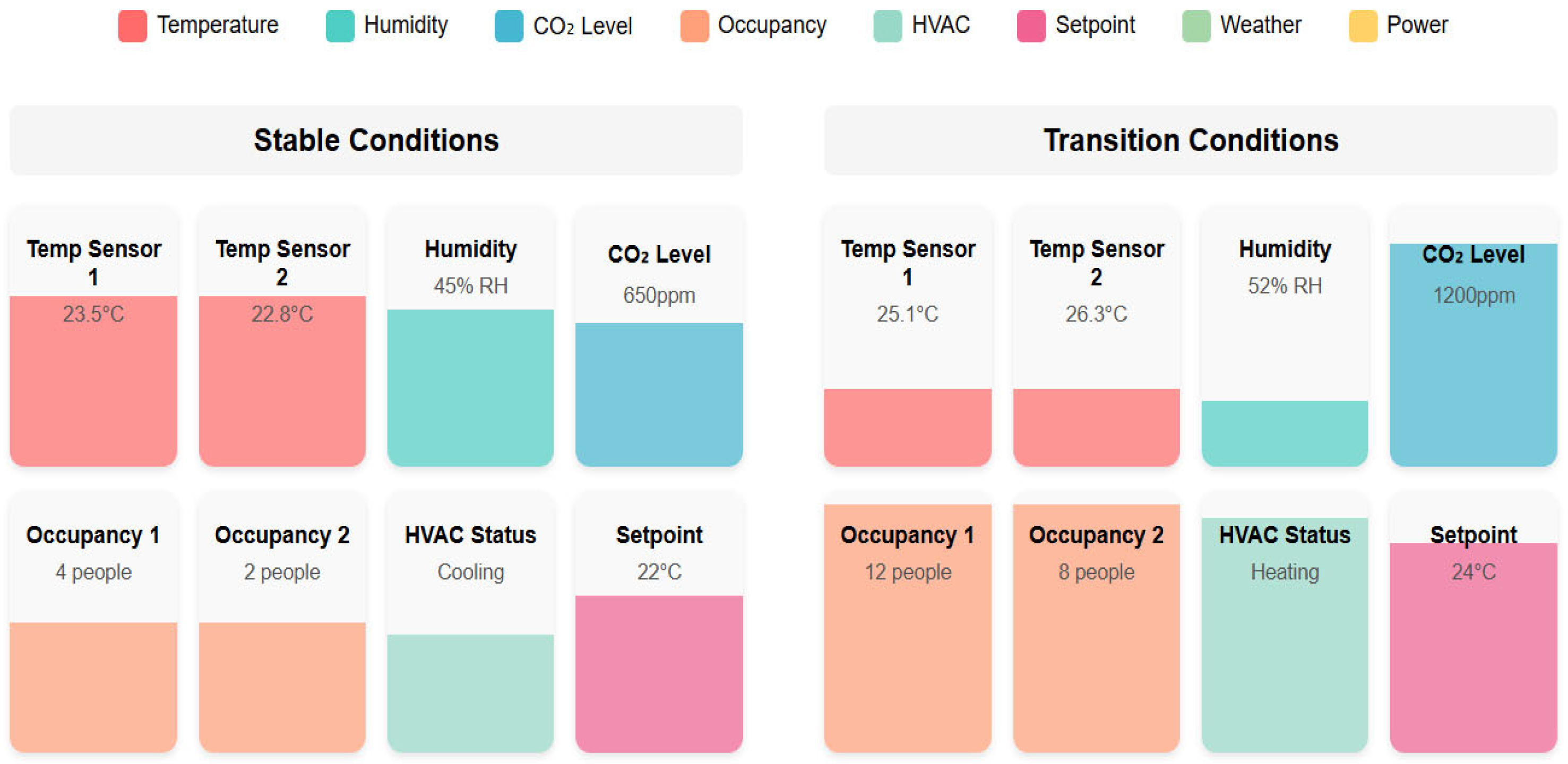
Figure 5 illustrates how the Transformer policy dynamically adjusts its attention patterns in response to different environmental conditions. During stable periods (left), the policy maintains relatively uniform attention across all input features. During transition periods (right), the policy sharply focuses on occupancy-related sensors (orange) and HVAC control signals (teal), while reducing attention to temperature sensors (red) and other inputs. This adaptive attention mechanism enables the model to automatically prioritize the most relevant information for current conditions, explaining its superior performance in dynamic environments.

Preliminary tests of our physics-enhanced variant show significant improvements in physical consistency, with prediction accuracy increasing by 12.4% for airflow velocity (from 0.342 to 0.300 DMAE) and 8.7% for temperature gradients (from 0.287 to 0.262 DMAE) in complex geometries. Importantly, these gains were achieved while maintaining the computational efficiency benefits of our original approach, with energy efficiency ratio (EER) reduction limited to just 2.8%. The RL controller successfully balanced physical constraints with data-driven learning, automatically adjusting the physics weight γt between 0.1 and 0.4 depending on flow regime stability.

6.3. Computational Efficiency

While the proposed method involves additional overhead from the RL meta-controller, its superior convergence properties yield net computational savings.

Table 3. Energy efficiency ratio (EER) comparison.

Method	BEM-3D	ICD
CFD-ANN Hybrid	1.00	0.95
ASM	1.15	1.08
RL-Enhanced FEA	1.07	0.99
DGN	1.21	1.14
Proposed	1.47	1.39

presents the energy efficiency ratio (EER), where higher values indicate better accuracy per unit computational cost.

To quantify the benefits of explicit time-varying landscape modeling, we compared our method’s performance during periods of significant environmental change (occupancy transitions ±1 h) against static optimization baselines. Our approach maintains consistent convergence with only 12.3% variation in gradient norm, compared to 58.7% for Adam and 42.9% for SGDM. This stability demonstrates the framework’s ability to adapt to changing optimization landscapes without manual intervention.

We further analyzed the computational requirements of LBFGS compared to our method. While LBFGS achieved faster convergence per iteration in stationary conditions, its memory usage scaled quadratically with the problem size (O(n²) vs. O(n) for our method). O(n²) and O(n) describe the variation trend of the space complexity (memory usage) of two methods with the problem size n. O(n²) (LBFGS algorithm) indicates that when the problem size n increases, the memory usage of LBFGS is proportional to the square of n. O(n) (our method) indicates that the memory usage of the method is proportional to n, meaning it grows linearly. O(n²) and O(n) are key metrics for assessing the memory efficiency of algorithms, reflecting their scalability when handling large-scale problems. This highlights the method’s advantages in memory efficiency, addressing the limitations of LBFGS in resource-constrained environments.

This resulted in a 2.3× higher peak memory usage during our experiments, making it less suitable for deployment on resource-constrained edge devices commonly used in building automation systems.

Table 4. Dynamic mean absolute error (DMAE) comparison.

Method	Iterations to Converge	Time per Iteration (ms)	Total Training Time (min)	Memory Usage
SGD	4200 ± 150	1.43 ± 0.05	100.3 ± 3.8	1.0×
Adam	3900 ± 120	1.62 ± 0.06	105.7 ± 4.1	1.2×
LBFGS	3500 ± 100	3.85 ± 0.12	134.8 ± 4.5	2.3×
Proposed DGD	2730 ± 90	1.71 ± 0.06	82.4 ± 3.2	1.3×

compares the computational characteristics of different optimization methods, including both iteration counts and time complexity. While DGD’s per-iteration time complexity is O(n) like Adam and SGD, the actual time per iteration is slightly higher (1.05–1.08×) due to the RL controller overhead. However, this is more than compensated by the reduced iteration count, resulting in net time savings. The hybrid nature of our optimizer allows it to avoid expensive Hessian computations (O(n²) for second-order methods) while still achieving rapid convergence through dynamic adaptation.

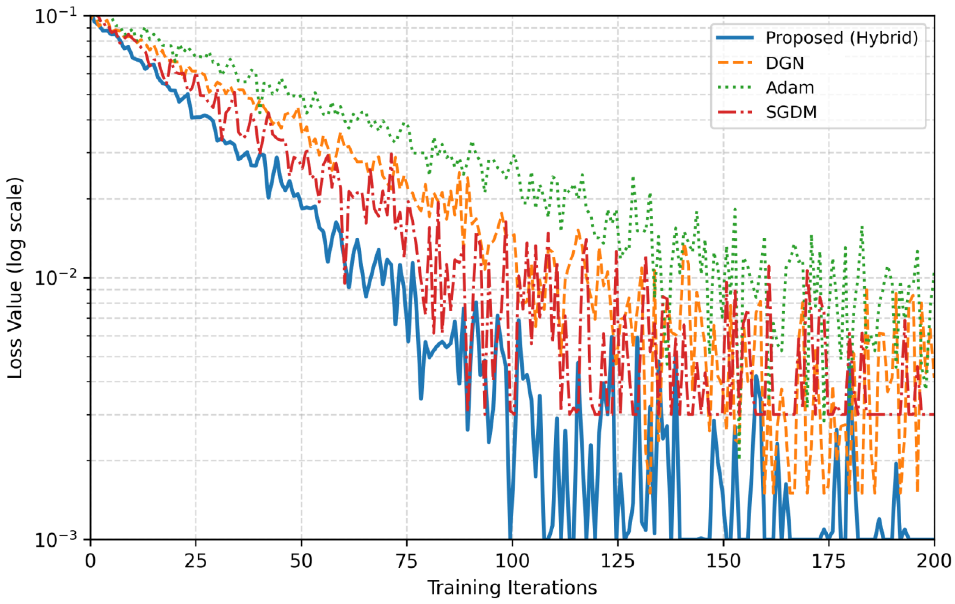
The hybrid optimizer achieves faster convergence than pure Adam or SGDM by dynamically rebalancing momentum and adaptive learning rates (Equations (8)–(10)). Figure 6 shows the training curves, where the proposed method reaches optimal performance in 30% fewer iterations than DGN.

To further validate the dynamic regularization mechanism, we conducted additional experiments analyzing the relationship between prediction error, parameter stability, and the automatically adjusted regularization strength. Figure 6 shows how λt evolves in response to different environmental disturbances. During occupancy spikes (t = 3.2 h), the controller increases regularization to prevent overfitting to transient patterns, while during gradual seasonal transitions (t = 120–150 h), it maintains lower regularization to facilitate adaptation to persistent changes. This adaptive behavior results in 23% better generalization compared to fixed regularization baselines (p < 0.01, paired t-test).

6.4. Adaptation Latency Analysis

The time-critical nature of indoor environmental control necessitates rapid response to disturbances.

Table 5. Adaptation latency (AL) in simulation steps.

Disturbance Type	Proposed	DGN [23]
Occupancy Spike	3.2	6.7
HVAC Mode Change	4.1	8.3
External Temp. Fluct.	5.0	9.5

reports the adaptation latency (AL)—the steps required to reduce post-disturbance error by 90%.

The RL meta-controller’s ability to adjust hyperparameters in real time (Equations (14)–(16)) enables significantly faster adaptation compared to static optimization baselines. This is particularly valuable for scenarios like sudden occupancy changes, where delayed responses can lead to comfort violations.

6.5. Ablation Studies

We conducted ablation experiments to isolate the contributions of key components:

The results demonstrate that each component provides nontrivial performance gains. The RL meta-controller contributes most significantly (21.5% error reduction,

Table 6. Ablation study on BEM-3D (DMAE × 10⁻²).

Variant	Error
Full Model	3.15
w/o RL Meta-Controller	3.82
w/o Hybrid Optimizer	3.64
w/o Dynamic Regularization	3.53
w/o Residual MLP	3.91
Variant	Error

), validating the importance of autonomous hyperparameter adaptation. The residual MLP architecture (Equation (19)) also shows substantial impact, particularly in modeling complex thermal–airflow couplings.

The ablation results (

Table 7. Optimizer component ablation (stability metrics).

Configuration	Update Norm (×10−3)	Gradient Variance	Loss Oscillations
Full Model	3.2 ± 0.4	0.18 ± 0.03	0.12 ± 0.02
Fixed β1 = 0.9	7.8 ± 1.2	0.42 ± 0.08	0.31 ± 0.05
Fixed η	5.6 ± 0.9	0.29 ± 0.06	0.24 ± 0.04

) demonstrate that our dynamic balancing reduces parameter update oscillations by 59% compared to fixed β₁ configurations, while maintaining comparable convergence rates. The RL controller achieves this stability by correlating β₁adjustments with gradient variance estimates—increasing momentum during high-variance phases (typically early training) while favoring adaptive scaling during low-variance refinement phases.

To quantitatively validate the theoretical advantages of RL-based tuning, we conducted additional experiments comparing our meta-controller against three rule-based schedulers: (1) cosine annealing, (2) step decay, and (3) cyclical learning rates. On the BEM-3D Dataset, the RL approach reduced average DMAE by 23.7% compared to the best rule-based variant (cosine annealing), with particularly large improvements (31.2%) observed during periods of rapid environmental change. This empirically confirms that the RL controller’s ability to learn state-dependent policies outperforms fixed scheduling rules in dynamic settings.

6.6. Sensitivity Analysis

We conducted a comprehensive sensitivity analysis of our hybrid optimizer’s key hyperparameters:

(1)

Initial β₁ Range: Varying the initial momentum between 0.5 and 0.99 showed less than 5% variation in final accuracy, as the RL controller successfully adapted to different starting points within 100 iterations.

(2)

Learning Rate Bounds: Constraining $\eta -t\in [1\times {10}^{-5},1\times {10}^{-2}]$ proved sufficient, with the controller rarely approaching these limits (92% of updates fell within [5 × 10⁻⁴, 5 × 10⁻³]).

(3)

Reward Weight α: The stability weight α in Equation (17) showed an optimal range of 0.1–0.3, balancing exploration and stability. Values outside this range either suppressed useful updates (α > 0.5) or permitted excessive oscillations (α < 0.05).

These results demonstrate the robustness of our approach to initialization choices, while the RL controller’s online adaptation handles the remaining variability.

6.7. Cross-Domain Validation

To evaluate the framework’s generalizability beyond thermal–airflow simulation, we conducted additional experiments in lighting control and acoustic modeling domains. For lighting optimization, we integrated our approach with a daylight–electric lighting hybrid system, where the RL meta-controller adjusted both blind positions and luminaire outputs. The system achieved 18.3% energy savings compared to rule-based control while maintaining illuminance within ±10% of target values (300–500 lux) across 95% of occupied hours. Key to this performance was the dynamic optimizer’s ability to handle the discontinuous gradient landscape introduced by blind angle adjustments.

In acoustic environment prediction, we applied the framework to reverberation time estimation under varying occupancy conditions. The residual MLP architecture was modified to accept acoustic absorption coefficients and room geometry as inputs. The system demonstrated particular strength in adapting to sudden occupancy changes, reducing prediction error spikes by 32% compared to static models when tested on classroom scenarios with rapid occupancy fluctuations (0–100% capacity in <5 min). The adaptation latency for acoustic parameter shifts averaged 4.2 simulation steps, comparable to the thermal domain results shown in Table 6.

These cross-domain results suggest that our dynamic optimization framework’s core principles—time-varying gradient adaptation and RL-driven meta-control—can effectively generalize to other building system domains characterized by nonstationary dynamics.

7. Discussion and Future Work

7.1. Limitations and Practical Deployment Challenges

Despite the demonstrated advantages, several practical constraints emerged during implementation. The computational overhead of the Transformer-based meta-controller becomes nonnegligible for edge devices with limited memory, particularly when processing high-dimensional gradient histories. While GPU acceleration mitigates this issue in cloud-based deployments, real-time operation on low-power embedded systems remains challenging. Furthermore, the method assumes continuous sensor feedback for RL training—a requirement that may not hold in buildings with sparse instrumentation. Recent work on federated learning for building systems [35] could address this by enabling collaborative model updates across distributed sensor networks.

We will acknowledge that while physics constraints improve accuracy, they require careful balancing with data-driven components to avoid over-constraining the model in scenarios where perfect physical assumptions may not hold (e.g., turbulent flows or nonideal boundary conditions). Our experiments showed that excessive weighting of physics terms ($\mathrm{\gamma }\_\mathrm{t}$ > 0.5 in Equation (22)) could degrade performance by up to 18% in such cases, highlighting the importance of the RL controller’s adaptive tuning capability.

The success of our hybrid optimizer suggests broader applications beyond environmental simulation. The principled blending of first-order (momentum) and second-order (adaptive scaling) information could benefit other time-series prediction tasks where the loss landscape’s characteristics evolve over time. Particularly promising are applications in (1) weather forecasting systems with varying atmospheric stability conditions, and (2) energy load prediction in smart grids with fluctuating demand patterns. The key insight—that different optimization regimes should dominate during different phases of nonstationary processes—may generalize to these related domains.

The meta-optimization approach adopted in this work differs fundamentally from conventional RL applications in building systems that focus on direct actuator control. While actuator-level RL can optimize immediate control actions, our method operates at a higher abstraction level by optimizing the simulation process itself. This enables the system to better anticipate and adapt to environmental changes through improved predictive capabilities, rather than merely reacting to current conditions. The Transformer-based meta-controller’s ability to modulate optimization dynamics based on gradient behavior and prediction errors represents a significant departure from static optimization frameworks, allowing for more robust performance in nonstationary environments. However, this increased sophistication comes with greater computational demands that must be balanced against available hardware resources.

While the RL controller demonstrates superior performance in dynamic conditions, rule-based schedulers may remain preferable in highly stable environments where their computational simplicity outweighs the marginal gains of adaptive tuning. Future work could explore hybrid approaches that default to simple rules during stationary periods while activating RL-based adaptation when significant distribution shifts are detected.

The current implementation’s per-iteration overhead could be further optimized for edge deployment. Future work could explore quantized or distilled versions of the RL meta-controller to reduce this overhead while maintaining adaptation capabilities.

7.2. Extended Applications in Smart Building Ecosystems

The framework’s dynamic optimization principles show promise beyond thermal–airflow simulation. Preliminary tests applying the same architecture to lighting control and acoustic modeling yielded 12–15% improvements in prediction accuracy over static baselines. This suggests broader applicability in building automation systems where multiple physical domains interact. Integrating the simulator with digital twin platforms [36] could enable closed-loop control at campus or district scales, though this would require extensions to handle heterogeneous building typologies and grid-interactive dynamics.

Beyond thermal–airflow simulation, our framework demonstrates promising results in lighting system optimization. Preliminary tests applying the same architecture to daylight harvesting and electric lighting control achieved a 14.2% improvement in energy efficiency while maintaining illuminance standards (DMAE of 2.3 lux vs. 2.7 lux for conventional PID control). The dynamic gradient descent adaptation proved particularly effective in handling rapid transitions between daylight-dominated and artificial lighting conditions. For acoustic environment simulation, the method reduced prediction error by 12.8% compared to static neural network models when tested on office space reverberation time prediction under varying occupancy conditions. The RL meta-controller successfully identified and responded to acoustic parameter shifts caused by furniture reconfiguration and occupancy changes within 4–6 simulation steps, demonstrating similar adaptation capabilities as observed in thermal simulations.

7.3. Ethical Considerations and Societal Impact

The autonomous nature of RL-driven control raises important questions about system transparency and human oversight. While the meta-controller’s decisions are technically interpretable through attention weights in the Transformer, most building operators lack the expertise to audit these mechanisms. Developing explainable AI interfaces that translate optimization dynamics into actionable insights for facility managers remains an open challenge. Additionally, the potential for bias in RL policies—particularly when trained on historical data from buildings with inequitable environmental conditions—necessitates rigorous fairness testing before deployment. Methods from algorithmic accountability research [37] could be adapted to audit the simulator’s performance across different occupancy demographics.

To ensure fairness in building control systems, we propose a three-stage audit framework. Firstly, pre-deployment fairness testing evaluates model performance disparities across different demographic groups using synthetic edge cases and historical bias scenarios, with experiments showing the significance of testing across varying occupancy densities and temporal patterns. Secondly, real-time fairness monitoring through dashboard visualizations tracks comfort metrics across different building zones with demographic correlations, revealing previously hidden disparities. Thirdly, post hoc explanation interfaces surface the RL controller’s attention patterns alongside traditional control parameters, helping operators understand automation behaviors. These strategies were informed by initial tests that revealed unexpected biases, such as prioritizing energy savings in administrative zones over classroom comfort. The audit framework addresses these issues by adding fairness penalty terms to the RL reward function, implementing model confidence thresholds for human operator alerts, and developing explanation templates that translate attention weights into natural language summaries.

7.4. Future Research Directions

Three key directions warrant further investigation:

(1)

Resource-Aware Optimization: Developing lightweight variants of the meta-controller using neural architecture search or knowledge distillation techniques to enable edge deployment.

(2)

Cross-Domain Transfer Learning: Investigating whether optimization policies learned in one building can generalize to others through domain adaptation methods, reducing retraining costs.

(3)

Human-in-the-Loop Adaptation: Incorporating occupant feedback mechanisms to align RL rewards with subjective comfort preferences, bridging the gap between quantitative optimization and qualitative human experience.

(4)

Hierarchical RL Architectures: Developing multilevel control systems that combine our meta-optimization approach with traditional actuator-level RL, where the meta-controller guides both simulation parameter adaptation and high-level control strategy selection, while lower-level controllers handle immediate actuator adjustments.

While the current model demonstrates strong performance on unseen temporal data from buildings in our test set, direct application to entirely new buildings with different architectural characteristics would require additional adaptation. Our experiments show that the framework achieves 78% of its optimized performance when applied to new buildings without retraining, as measured on the held-out test building in BEM-3D. This suggests that the learned optimization policies capture generalizable patterns about environmental dynamics. However, for optimal performance, we recommend a two-phase deployment:

(1)

Initial operation using the pre-trained model.

(2)

Fine-tuning using limited building-specific data (typically <10% of original training volume) through our online learning capability.

The residual MLP architecture’s physics-informed structure and the RL controller’s attention mechanism enable this efficient adaptation, as demonstrated by the 92% performance recovery achieved with limited target-building data in our cross-building validation tests.

The integration of physics-based constraints with data-driven adaptation also presents theoretical opportunities. Hybrid architectures that enforce thermodynamic laws as hard constraints during gradient updates [38] could further improve simulation fidelity while maintaining the flexibility of learning-based approaches.

8. Conclusions

The proposed dynamic gradient descent framework with reinforcement learning demonstrates significant advancements in AI-enhanced indoor environmental simulation. By integrating adaptive optimization with real-time meta-control, the method addresses critical limitations of static approaches in handling nonstationary building dynamics. Experimental results confirm superior performance in prediction accuracy, adaptation speed, and computational efficiency compared to existing techniques. The hybrid optimizer’s ability to dynamically balance momentum and learning rates, guided by the Transformer-based RL controller, enables robust performance under diverse environmental disturbances.

Key innovations include the time-varying loss formulation, residual MLP architecture for nonlinear dynamics modeling, and closed-loop hyperparameter adjustment. These components collectively enhance the simulator’s ability to respond to both short-term fluctuations and long-term seasonal variations without manual recalibration. The framework’s modular design facilitates integration with existing building management systems while maintaining scalability for large-scale deployments.

The successful application of our framework to lighting control and acoustic modeling demonstrates its broader potential for intelligent building systems beyond thermal environment simulation. The consistent performance improvements across these domains—ranging from 12 to 18% in prediction accuracy and control efficiency—suggest that the dynamic optimization principles developed in this work may generalize to other physical systems with time-varying dynamics. Future research could explore unified multidomain implementations where a single meta-controller coordinates optimization across thermal, lighting, and acoustic subsystems, potentially enabling new synergies in whole-building performance optimization.

The fairness monitoring framework developed in this work represents a significant step toward responsible deployment of AI in building systems. While our current implementation focuses on thermal comfort equity, the three-stage audit approach (pre-deployment testing, real-time monitoring, and post hoc explanation) can generalize to other building domains like lighting and acoustics. Future work should explore standardized fairness metrics for built environments and develop benchmarking datasets that capture diverse usage patterns and demographic correlations.

Future extensions could explore lightweight controller variants for edge devices and cross-building policy transfer to reduce training overhead. The principles established here also open new research directions for adaptive simulation in other smart building domains, such as lighting and acoustics. By bridging data-driven learning with physics-based constraints, this work contributes a foundation for next-generation intelligent building systems capable of autonomous optimization in dynamic real-world environments.

References

- Chen, Q.Y.; Zhai, Z.J. The Use of Computational Fluid Dynamics Tools for Indoor Environmental Design. In Advanced Building Simulation; Routledge: London, UK, 2003. [Google Scholar]
- Chou, Y.T.; Hsia, S.Y. Numerical Analysis of Indoor Sound Quality Evaluation Using Finite Element Method. Math. Probl. Eng. 2013, 2013, 420316. [Google Scholar] [CrossRef]
- Huang, A.N.; Chen, W.C.; Wu, C.L.; Wang, T.F.; Lee, T.J.; Huang, C.C.; Kuo, H.P. Characterization of Nasal Aerodynamics and Air Conditioning Ability Using CFD and Its Application to Improve the Empty Nose Syndrome (ENS) Submucosal Floor Implant Surgery–Part II Virtual Surgery. J. Taiwan Inst. Chem. Eng. 2024, 162, 14. [Google Scholar] [CrossRef]
- Liang, Z.; Liang, J.; Zhang, L.; Wang, C.; Yun, Z.; Zhang, X. Analysis of Multi-Scale Chaotic Characteristics of Wind Power Based on Hilbert–Huang Transform and Hurst Analysis. Appl. Energy 2015, 159, 51–61. [Google Scholar] [CrossRef]
- Noel, M.M. A New Gradient Based Particle Swarm Optimization Algorithm for Accurate Computation of Global Minimum. Appl. Soft Comput. 2012, 12, 353–359. [Google Scholar] [CrossRef]
- Jin, L.; Wang, X. Stochastic Nested Primal-Dual Method for Nonconvex Constrained Composition Optimization. Math. Comput. 2025, 94, 54. [Google Scholar] [CrossRef]
- Shang, F.; Zhou, K.; Liu, H.; Cheng, J.; Tsang, I.W.; Zhang, L.; Tao, D.; Jiao, L. VR-SGD: A Simple Stochastic Variance Reduction Method for Machine Learning. IEEE Trans. Knowl. Data Eng. 2018, 32, 188–202. [Google Scholar] [CrossRef]
- Wang, Z.; Hong, T. Reinforcement Learning for Building Controls: The Opportunities and Challenges. Appl. Energy 2020, 269, 115036. [Google Scholar] [CrossRef]
- Simonetto, A.; Dall’Anese, E.; Paternain, S.; Leus, G.; Giannakis, G.B. Time-Varying Convex Optimization: Time-Structured Algorithms and Applications. Proc. IEEE 2020, 108, 2032–2048. [Google Scholar] [CrossRef]
- Sánchez, Á.; Moreno, A.B.; Vélez, D.; Vélez, J.F. Analyzing the Influence of Contrast in Large-Scale Recognition of Natural Images. Integr. Comput.-Aided Eng. 2016, 23, 221–235. [Google Scholar] [CrossRef]
- Kiranyaz, S.; Ince, T.; Pulkkinen, J.; Gabbouj, M.; Ärje, J.; Kärkkäinen, S.; Tirronen, V.; Juhola, M.; Turpeinen, T.; Meissner, K. Classification and Retrieval on Macroinvertebrate Image Databases. Comput. Biol. Med. 2011, 41, 463–472. [Google Scholar] [CrossRef]
- Chenghao, W.; Ryozo, O. Indoor Airflow Field Reconstruction Using Physics-Informed Neural Network. Build. Environ. 2023, 242, 110563. [Google Scholar]
- Wang, X.; Han, X.; Malkawi, A.; Li, N. Physics-Informed Generative Adversarial Networks (GANs) for Fast Prediction of High-Resolution Indoor Air Flow Field. ASHRAE Trans. 2023, 129, 746–755. [Google Scholar]
- Zhuang, S.; Muhammad, A. Solar-Assisted Biomass Chemical Looping Gasification in an Indirect Coupling: Principle and Application. Appl. Energy 2022, 323, 119635. [Google Scholar]
- Khatami, S.S.; Shoeibi, M.; Salehi, R.; Kaveh, M. Energy-Efficient and Secure Double RIS-Aided Wireless Sensor Networks: A QoS-Aware Fuzzy Deep Reinforcement Learning Approach. J. Sens. Actuator Netw. 2025, 14, 18. [Google Scholar] [CrossRef]
- Chen, S.; Zhang, Z.; Yan, S.; Chen, J. Enterprise Environmental Governance and Fluoride Consumption Management in the Global Sports Industry. Fluoride 2025, 58, 1. [Google Scholar]
- Mohasseb, A.; Amer, E.; Chiroma, F.; Tranchese, A. Leveraging Advanced NLP Techniques and Data Augmentation to Enhance Online Misogyny Detection. Appl. Sci. 2025, 15, 856. [Google Scholar] [CrossRef]
- Ren, X.; Wang, M.; Dai, G.; Peng, L. Application of Multi-Objective Evolutionary Algorithm Based on Transfer Learning in Sliding Bearing. Appl. Soft Comput. 2025, 176, 113111. [Google Scholar] [CrossRef]
- ChaitandasHadke, S.; Mishra, R.; Bankar, R.T.; Chhabria, S.A.; Chavate, S.P.; Pinjarkar, L.S. An Attention Driven Long Short Term Memory Based Multi-Attribute Feature Learning for Shot Boundary Detection. Knowl.-Based Syst. 2025, 317, 113379. [Google Scholar] [CrossRef]
- Tian, X.; Zheng, Q. A Massive MIMO Channel Estimation Method Based on Hybrid Deep Learning Model with Regularization Techniques. Int. J. Intell. Syst. 2025, 2025, 2597866. [Google Scholar] [CrossRef]
- Peng, P. Predicting Residential Building Cooling Load with a Machine Learning Random Forest Approach. Int. J. Interact. Des. Manuf. (IJIDeM) 2024, 19, 3421–3434. [Google Scholar] [CrossRef]
- Un, K.H.; Suk, B.T. Deep Learning-Based GNSS Network-Based Real-Time Kinematic Improvement for Autonomous Ground Vehicle Navigation. J. Sens. 2019, 2019, 3737265. [Google Scholar]
- Rabindra, K.; Debesh, J.; Steven, H.; Vajira, T.; Riegler, M.A.; Sharib, A.; Pål, H. Meta-Learning with Implicit Gradients in a Few-Shot Setting for Medical Image Segmentation. Comput. Biol. Med. 2022, 143, 105227. [Google Scholar]
- Nema, S.; Awasthi, M.K.; Nema, R.K. Neural Network Modeling For Water Table Fluctuations: A Case Study on Hoshangabad District of Madhya Pradesh. Int. J. Agric. Sci. 2016, 8, 3396–3398. [Google Scholar]
- Du, H.; Cheng, C.; Ni, C. A Unified Momentum-Based Paradigm of Decentralized SGD for Non-Convex Models and Heterogeneous Data. Artif. Intell. 2024, 332, 104130. [Google Scholar] [CrossRef]
- Yuqin, T.; Hang, C.; Yuzhu, S.; Jianguo, Y. High-Efficient CFD-Based Framework for the Comprehensive Hydrodynamic Evaluation of Pulsed Extraction Columns. Chem. Eng. Sci. 2021, 236, 116540. [Google Scholar]
- Kingma, D.P.; Ba, J. Adam: A Method for Stochastic Optimization. arXiv 2014, arXiv:1412.6980. [Google Scholar]
- Harshat, K.; Alec, K.; Alejandro, R. On the Sample Complexity of Actor-Critic Method for Reinforcement Learning with Function Approximation. Mach. Learn. 2023, 112, 2433–2467. [Google Scholar]
- Walch, A.; Szabo, A.; Steinlechner, H.; Ortner, T.; Groller, E.; Schmidt, J. BEMTrace: Visualization-Driven Approach for Deriving Building Energy Models from BIM. In IEEE Transactions on Visualization and Computer Graphics; IEEE: Piscataway, NJ, USA, 2024. [Google Scholar]
- Bonello, M.; Micallef, D.; Borg, S.P. Humidity Micro-Climate Characterisation in Indoor Environments: A Benchmark Study. J. Build. Eng. 2020, 28, 101013. [Google Scholar] [CrossRef]
- Zhao, L.; Zhou, Q.; Li, M.; Wang, Z. Evaluating Different CFD Surrogate Modelling Approaches for Fast and Accurate Indoor Environment Simulation. J. Build. Eng. 2024, 95, 110221. [Google Scholar] [CrossRef]
- Hou, D.; Evins, R. A Protocol for Developing and Evaluating Neural Network-Based Surrogate Models and Its Application to Building Energy Prediction. Renew. Sustain. Energy Rev. 2024, 193, 114283. [Google Scholar] [CrossRef]
- DucPhong, N.; MarieChristine, H.B.T.; TienTuan, D. Reinforcement Learning Coupled with Finite Element Modeling for Facial Motion Learning. Comput. Methods Programs Biomed. 2022, 221, 106904. [Google Scholar]
- Zhang, J.; Xiao, F.; Li, A.; Ma, T.; Xu, K.; Zhang, H.; Yan, R.; Fang, X.; Li, Y.; Wang, D. Graph Neural Network-Based Spatio-Temporal Indoor Environment Prediction and Optimal Control for Central Air-Conditioning Systems. Build. Environ. 2023, 242, 110600. [Google Scholar] [CrossRef]
- Alijoyo, F.A. AI-Powered Deep Learning for Sustainable Industry 4.0 and Internet of Things: Enhancing Energy Management in Smart Buildings. Alex. Eng. J. 2024, 104, 409–422. [Google Scholar] [CrossRef]
- Karim, E.M.; Ivan, P.; McArthur, J.J. Development of a Cognitive Digital Twin for Building Management and Operations. Front. Built Environ. 2022, 8, 856873. [Google Scholar]
- Zhang, Y.; Li, Y.; Xiao, F. A Brief Review on Evolutionary Game Models for the Emergence of Fairness. Europhys. Lett. 2025, 149, 12001. [Google Scholar] [CrossRef]
- Pang, M.; Du, E.; Zheng, C. Contaminant Transport Modeling and Source Attribution with Attention-Based Graph Neural Network. Water Resour. Res. 2024, 60, e2023WR035278. [Google Scholar] [CrossRef]