Building Fire Location Predictions Based on FDS and Hybrid Modelling

Abstract

With the goal of addressing the difficulty of rapidly identifying the source of fire in commercial buildings, this study builds a numerical fire model based on the fire dynamics simulator (FDS) and combines it with a hybrid model to predict the location of a fire source. Different scenarios were built to simulate the spatial and temporal distributions of key parameters such as temperature, smoke, and CO concentration during the fire process. Combining convolutional neural networks (CNNs) and support vector machines (SVMs) for prediction, the fire-source location prediction model with temperature, smoke, and CO concentration as feature quantities was constructed, and the hyperparameters affecting the model accuracy and generalisation were optimised by the Crested Porcupine Optimizer (CPO) algorithm. The experimental results show that the positioning error of this method under the building plane is less than 0.95 m, the mean absolute error (MAE) is within 0.35, and the root-mean-square error (RMSE) is within 0.41, which are 43% and 82% higher than the unoptimised model, respectively. The localisation accuracy of the fire-source room is 97.61%. In addition, the model’s anti-interference performance was tested under various extreme conditions. The results show that the proposed model can ensure the accurate location of a fire source and can provide information in emergencies.

1. Introduction

With the acceleration of global urbanisation, buildings are becoming increasingly large and structurally complex, and fire, as a common disaster, poses a serious threat to the safe management of buildings and the lives and property of people [1,2,3]. After a fire occurs, timely and accurate location of the fire source is the key to effectively extinguishing the fire and reducing casualties and property damage [4,5]. Rapid and accurate identification of the position of the fire source can curb the spread of fire, optimise the evacuation path, and enhance rescue efficiency [6]. However, with the increase in building scale and the diversity of fire propagation paths, it has been difficult to meet the needs of modern building fire emergency response using traditional fire-source localisation methods [7]. Such traditional fire-source location methods mainly include empirical judgement methods, methods based on data analysis, and thermal imaging technology [8]. The empirical method is the most traditional and easiest way to locate a fire source. Firefighters judge the possible location of the fire source by the fire scene (e.g., the direction of the fire spread, the direction of smoke flow, the area where the fire occurred, etc.). However, due to the complex environment of fire scenes, it is difficult to accurately determine the location of the fire source by intuition or experience, and it is dangerous for the rescuers. The method based on data analysis mainly involves analysing data from sensors such as smoke detectors, temperature sensors, and flame detectors (e.g., smoke concentration, temperature change, etc.), and combining them with the response of the fire alarm system to preliminarily determine the location of the fire source. However, in complex building structures, data from a single sensor often cannot provide accurate fire-source localisation, and it may be affected by factors such as the building environment and sensor layout, leading to localisation errors. Problems such as large positioning delay and weak anti-interference ability are common in complex building environments, making it difficult to meet the real-time demands of dynamic fire scenarios [9]. Thermal imaging technology determines the location of the fire source by measuring the thermal radiation in the fire area [10]. In the event of a fire, the fire source usually emits a large amount of heat, and this heat will cause the temperature of the surrounding environment to rise abnormally. Thermal imagers are able to capture these areas of temperature abnormality, thus helping to determine the location of the fire source. However, there are limitations to their accuracy and reliability due to the diffusion of heat and interference signals from other heat sources within the building.

Currently, there are methods for calculating fire risk in international standards, such as BS EN 13501-2:2023; Fire classification of construction products and building elements and ISO 16732-1:2012; Fire safety engineering. Fire risk assessment-General under the European Standard System, NFPA 551; Guide for the Evaluation of Fire Risk Assessments under the U.S. Standard System, and SFPE’s “Fire Protection Engineering Handbook”, etc. [11,12,13]. The NFPA can use event tree analysis (ETA) and fault tree analysis (FTA) in combination with an expert method for constructing a fire progression pathway. SFPE provides a quantitative risk calculation model based on Fire Dynamics Simulation (FDS). Methods for calculating fire risk can be categorised into three types: quantitative analysis, qualitative assessment, and mixed methods. Quantitative analysis methods can use event tree analysis, which starts from the initial fire source and simulates branching paths such as flame spread, smoke diffusion, and personnel response in a time series to calculate the probability of each node. The risk matrix approach and the checklist approach can be used in qualitative assessment, and mixed methods may use dynamic risk assessment based on machine learning, combining historical data to optimise risk thresholds. In addition, methods vary in different scenarios, such as individual risk calculation in public buildings and potential risk calculation in industrial facilities [14,15,16].

In fire research, the advantages of the traditional experiments described above are that they can demonstrate the fire development process more intuitively, with high data reliability, and can provide specific quantitative descriptions of fire characteristics. The experimental study simulates the whole process of a building fire, uses monitoring equipment to explore the relationship between key factors such as fire occurrence and smoke dispersion, and then obtains actual data for theoretical analysis. However, experimental research also has some limitations, mainly in the following areas:

• The high cost of the experiment. Fire experiments are often destructive and require actual buildings to reproduce the fire process, and especially for large buildings, this is more expensive. In addition, the actual source of the fire and its uncertainty, the slightest carelessness, will lead to danger.
• The experimental scene is difficult to reproduce. Due to the many uncertainties involved in the fire process, real fire situations are usually dynamic and complex. Even under the same experimental conditions, it is difficult to achieve accurate reproduction of the whole fire process.
• Narrow coverage of experimental research. Experimental studies cannot cover all possible fire scenarios, and their scope of application is somewhat limited. It is difficult to conduct comprehensive coverage of each fire condition, especially for experiments involving larger-scale buildings or extreme fire conditions.

Although experimental studies play an irreplaceable role in fire science research, they are limited by high cost, non-repeatability, and limitations in the settings of working conditions. The emergence of computer numerical simulation provides more possibilities for fire research and is becoming more and more important in modern building fire research. Numerical simulation can not only predict fire behaviour efficiently and cost-effectively but also provide flexible experimental design under various assumptions, thus making up for the shortcomings of traditional experimental research and promoting the development of fire science research.

As a result, this paper employs Revit technology combined with the fire dynamics simulator (FDS) to construct a fire database [17,18]. The combination of numerical simulation and a hybrid modelling approach can reduce the cost of installation and maintenance of hardware, wiring, and manpower in a fire detection system, and the data from numerical simulation and fire experiments is compared and analysed to ensure feasibility [19]. Combined with the data-driven approach, the model can be trained with a large amount of data to enable it to make accurate predictions of the location of the fire source.

Kevin modelled tunnel fires based on FDS and compared them with full-size tunnel experiments [20]. Bin proposed a Gaussian model and a multi-artificial fish school fusion algorithm to predict the location of the fire source in tunnel fires and carried out two extensive tunnel fire experiments [21]. Prabhash studied emergency passenger evacuation strategies using double-decker trains as simulation objects [22]. Liu simultaneously estimated the location of the fire source and its characteristics by applying a particle swarm optimisation technique to the multi-fire source identification problem [23]. Kou used a gated recurrent unit (GRU) to estimate the ignition chamber location for steady-state fires in multi-room buildings and compared it with a traditional recurrent neural network (RNN) approach [24]. Wu built a large database of tunnel fires and trained the data using the LSTM algorithm to improve the accuracy of ignition source localisation for tunnel fires [25]. F.L. used FDS and FEA to analyse RC structures subjected to temperature fields [26]. There are also intelligent methods, such as multi-method fusion prediction [27,28]. Yu combined various optimisation algorithms on the basis of the CNN model to form a novel hybrid framework, which not only realised the strength prediction of cement mortar in a sulphate environment but also applied to the research into the identification of automatic defects in a bridge deck [29,30].

In summary, it can be seen that FDS has demonstrated its excellent adaptability and flexibility in various types of building fire simulation, not only in accurately simulating the spread of fire and smoke distribution in a variety of building environments, but also in integrating with a variety of software platforms to form a powerful simulation and analysis system. However, the above studies mostly incorporate fire-source localisation in small-space planar scenarios such as tunnels and multi-modal buildings; the model has limitations in complex large-space environments and lacks a high degree of dimensionality awareness. In addition, the research is insufficient to verify the model’s generalisation and robustness in extreme situations, and the model’s ability to generalise across scenarios is limited by the absence of testing in extreme scenarios, such as high-temperature interferences and sensor failures in the building.

With the above analysis, this study aims to develop a prediction method based on FDS [31] and hybrid modelling [32] for enabling fire-source localisation in large commercial buildings. A building fire-source localisation system was constructed by deeply integrating geometric data from BIM, multi-physics field data from FDS simulation, and machine-learning methods [33]. Numerical simulations were validated by single-chamber fire experiments to demonstrate the realistic feasibility of numerical simulations. On this basis, a high realistic numerical simulation dataset was constructed. For model parameter selection, the CPO algorithm was introduced to achieve simultaneous optimisation of key parameters of the CNN-SVM using the dynamic neighbourhood search strategy of the porcupine defence mechanism to avoid local optima [34]. A hybrid CPO-CNN-SVM model was constructed to achieve high-precision fire location. The CPO-CNN-SVM model was also tested for its performance in various aspects to verify its adaptability and stability in complex and extreme environments. The contributions of the study are mentioned below:

• Numerical fire simulation validation was carried out to ensure the authenticity of the exogenous dataset and the feasibility of the experiment.
• Numerical models of real fires were constructed based on numerical simulations of fires, and the grid independence test was carried out to determine the optimal grid size by using the nested grid method. Numerical models were built to simulate various complex working conditions.
• The CPO-CNN-SVM fire-source localisation model was constructed, which is a hybrid model that incorporates the feature extraction advantages of CNN, and the Crested Porcupine Optimizer optimisation algorithm optimises the CNN-SVM hyperparameters to avoid unnecessary searching in the solution space and enhance the model performance.
• The CPO-CNN-SVM model was experimented with under multiple operating conditions (18 fire location scenarios), and the results show that the model performs well in terms of fire-source localisation.

This study aims to utilise FDS numerical simulation combined with machine-learning methods to achieve an accurate location of fire sources in commercial buildings. Through numerical simulation to circumvent the risk of real fire experiments, a variety of conventional working conditions and extreme conditions were simulated, and the robustness of the model was verified. The accurate and fast prediction of 2D position coordinates of the fire source for reference in fire rescue was realised. In addition to this, the model predictions were extended from fire-source coordinates to fire-source room localisation. FDS preset fires were used to generate training data to establish physical associations between combustion patterns and spatial features. Different locations and structures in each room generated unique temperature propagation patterns, forming differentiated timing features. The machine-learning model learned generalised mapping from temperature timings to room identifiers that can be directly applied to new buildings after training.

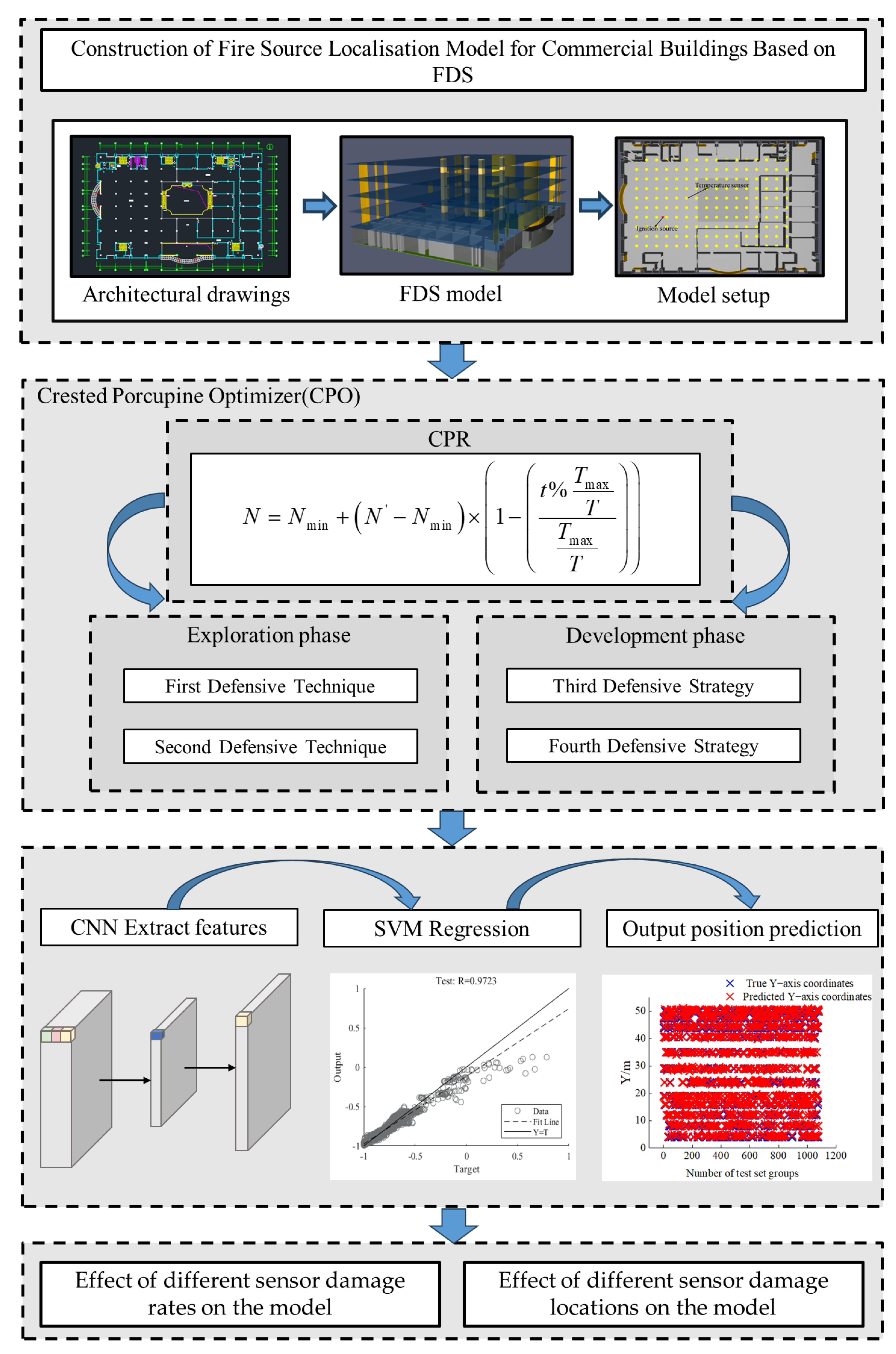
Figure 1 illustrates the technical route of this paper. The remainder of the paper is organised as follows: Section 2 presents the numerical simulation validation and modelling of commercial building fires; Section 3 describes the study of fire-source location modelling in commercial buildings; Section 4 presents the results of fire-source location prediction as well as the analysis of the model’s immunity to interference; and Section 5 gives the conclusions of the paper.

2. Numerical Simulation Validation and FDS Modelling

This paper simulates a retail atrium mall located in Dongguan City, Guangdong Province. Referring to the International Code of Building Classification ICC I-CODE IBC-2021, commercial buildings belong to the category of public buildings, but with special characteristics. Commercial buildings are mainly used for commodity trading, service provision, or business activities. Compared with schools, hospitals and other public buildings, they pay more attention to profitability and efficiency of crowd gathering. This retail mall is characterised by a special spatial structure, generally with a large open space. Commodity concentration leads to combustible distribution, which has certain characteristics. Holiday traffic causes an instantaneous surge. The layout of the floors is basically the same, except for the first floor. The third floor is the main location where experiments and data collection were conducted for this paper.

2.1. Single-Room Fire Verification

Numerical simulations have the advantage of low installation and maintenance costs and can be modelled in three dimensions based on the original drawings of the building and the properties of the main components. The purpose of their validation is to demonstrate the reliability of the fire dynamics simulation and to verify the correctness of the obtained data in cases where it is not possible to carry out real fire experiments to scale or in full size. The combination of numerical simulation and hybrid machine-learning models trained on a large amount of data allows for obtaining accurate results for temperature field analysis and fire location prediction.

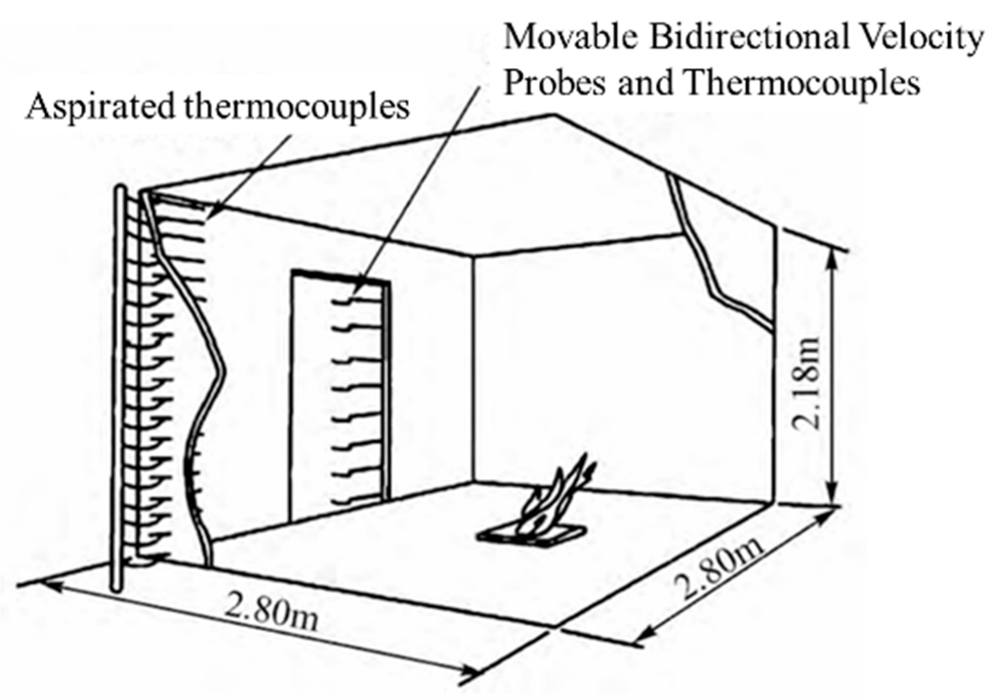
To ensure the realism of the training data, the simulation results of the numerical model were validated in this study in multiple steps. Steckler conducted a single-room fire test in 1982, in which comprehensive and detailed measurements of room temperature, doorway temperature, and doorway air flow rate were made for different fire-source locations and heat release rates, and the experimental room measured 2.8 m × 2.8 m × 2.13 m and contained a 1.83 × 0.74 m doorway as its vent. The room door dimensions, fire-source location, and heat release rate had a series of variations in the experiment, as shown in Figure 2 [35].

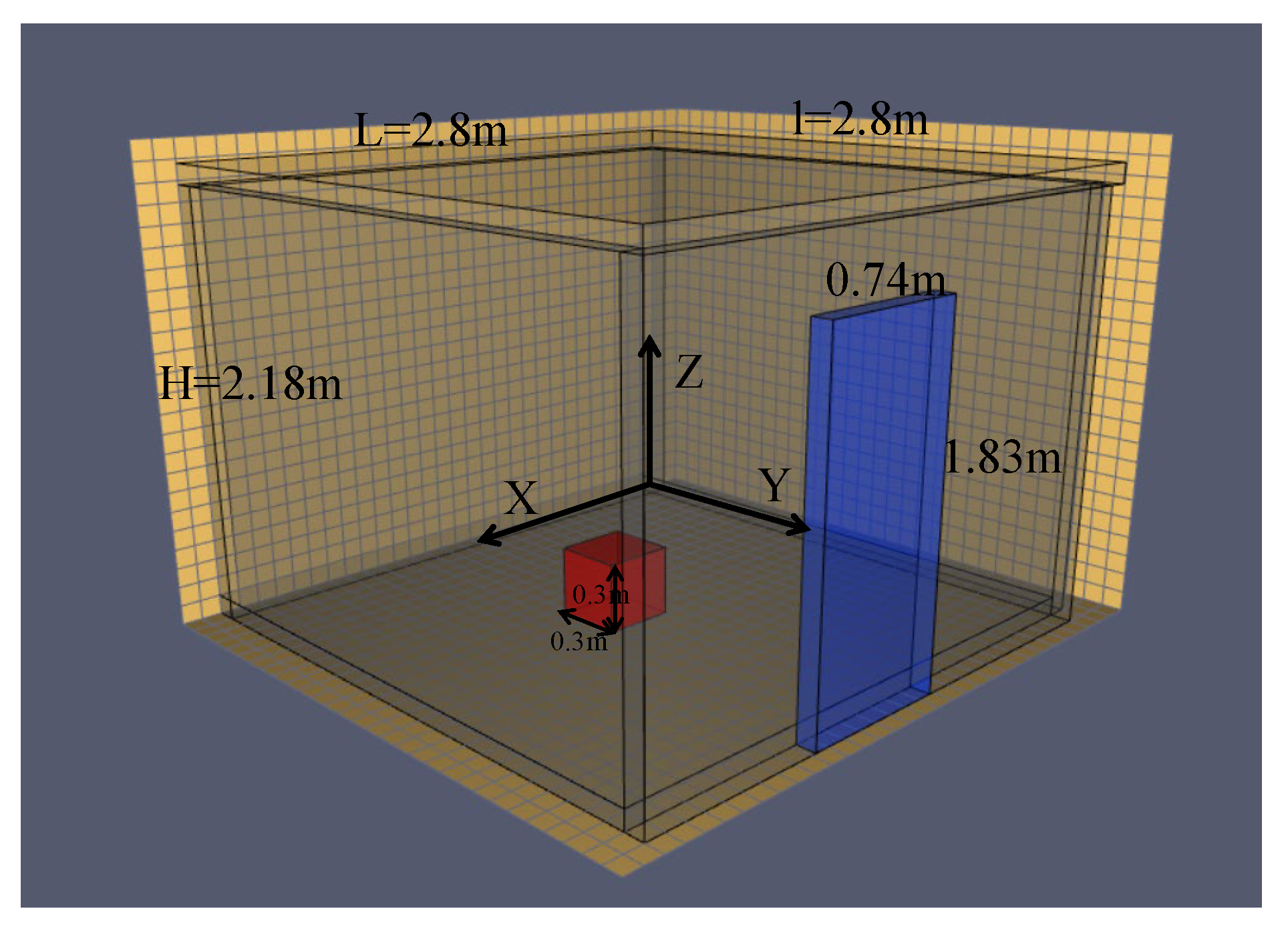
The power of the fire source was variously measured at 31.6 kW, 62.9 kW, 105.3 kW, and 158 kW. The size of the doorway opening varied from 0.24 to 0.99 m, and the height of the doorway was 1.83 m. Two-dimensional bi-directional velocity probes and bare-wire thermocouple arrays were arranged at the doorway to measure the flow velocity and temperature of the air at the doorway, with the vertical spacing of 0.114 m, where the first measurement point was 0.057 m from the floor. At the same time, to measure the temperature distribution at the corners of the room, a series of variations of the fire-source location and heat release rate were performed. To measure the temperature distribution at the corners of the room, a row of inhalation thermocouples was set up at the corners of the room, with thermocouple measurement points 0.305 m from each side wall, and a total of 19 thermocouples containing a thermocouple tree placed next to the front wall. The wall setup of the simulated room walls and ceiling was carried out based on the experimental description. The minimum grid size was 0.01 m, and the maximum was 0.05 m. The total grid size was 1.37 million, and the test room was connected to the outside space through a ‘door’ at an ambient temperature of 28 °C. The walls and ceiling were set up with ceramic fibre insulation boards to create quasi-steady state conditions. There were many kinds of working conditions because the fire-source location, fire-source heat release rate, and door opening size varied in the test. For this paper, we mainly simulated four working conditions in the test, and their parameter setting is shown in

Table 1. Parameter setting for different working conditions.

Working Condition	Location of Fire Source	Heat Release Rate/kW	Opening for Ventilation
1	A	62.9	Door: 1.83 m high and 0.74 m wide
2	B	105.3	Door: 1.83 m high and 0.74 m wide
3	C	62.9	Window: 0.92 m high, 0.74 m wide
4	A	31.6	Door: 1.83 m high and 0.74 m wide

. The corresponding FDS model of working condition 1 is shown in Figure 3, and the fire-source position and vent setting for each working condition are shown in Figure 4 and Figure 5.

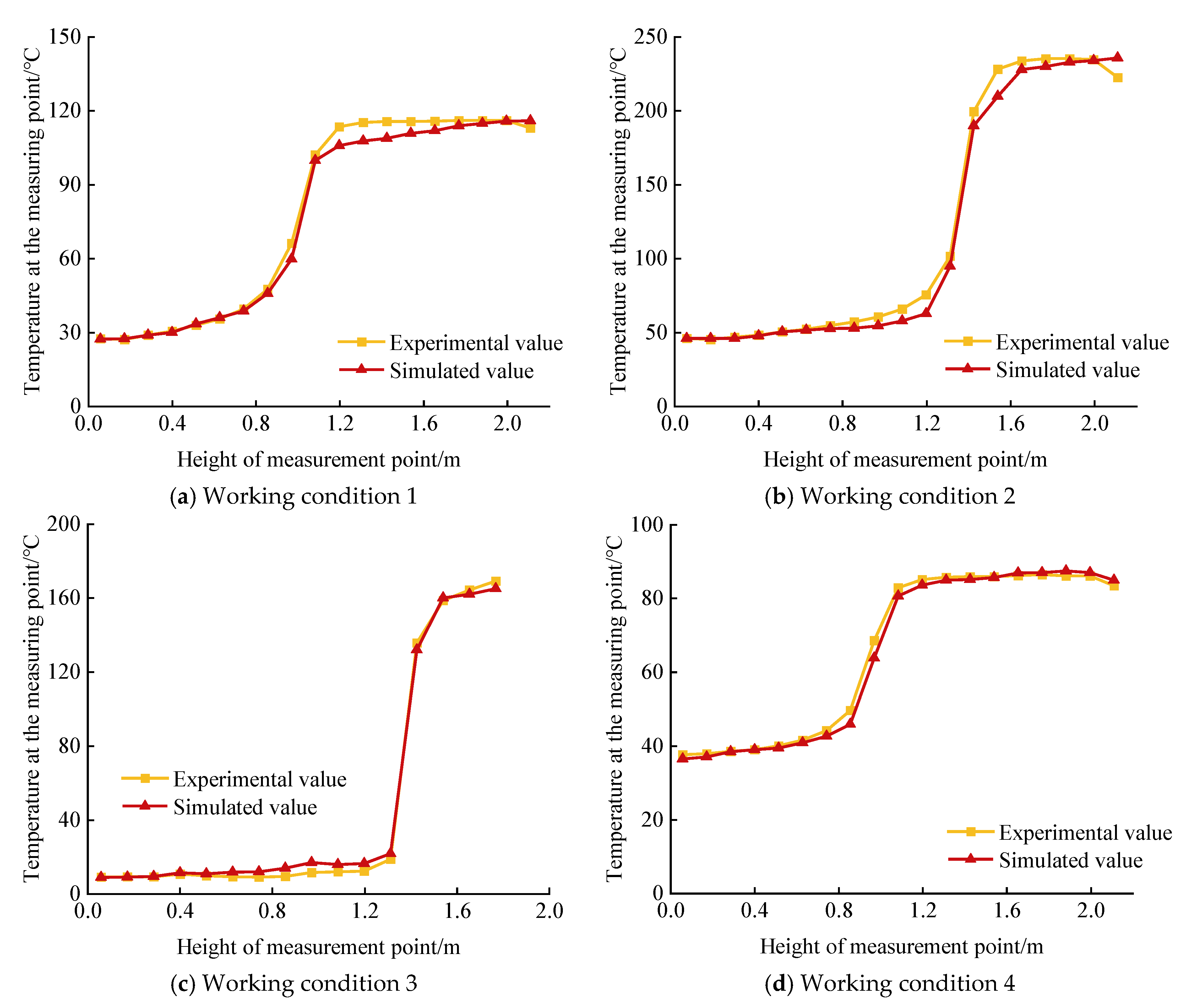
As the fire source will reach a steady state after ignition for a period of time, the temperature and velocity of the measurement point will also tend to level off after the fire source reaches a steady state; for example, in case 1, the temperature and velocity of the measurement point in the middle of the room door will reach the steady state after 50–80 s. To ensure that the simulation results are in the steady state, this paper selects the simulation results after 100 s and takes the average of the simulation results from 100–200 s as the final simulation result. The simulation results are compared and analysed with the test values. The comparison between the simulated and experimental values is shown in Figure 6.

From the analysis results of the Steckler fire test, it can be seen that the air temperature at the middle of the room and door and the temperature at the corners of the room obtained from the FDS simulation are closer to the test results, both in terms of trend and value, and in the case of the location of the fire source, the rate of heat release from the fire source and the dimensions of the ventilation openings are constantly changing.

2.2. Numerical Simulation of Commercial Building Fires

After obtaining the original drawings of the building, we set the floor heights, wall positions, and vent dimensions (e.g., window and door opening widths and heights) according to the design dimensions on a floor-by-floor basis and built the model in Pyrosim 2019 to generate a three-dimensional building geometric structure. At the same time, we set up various parameters and analysis indexes, including floor height, building dimensions, vent dimensions, etc.; defined the fire resistance level and thermophysical parameters of walls, floors, and other components; input the heat release rate (HRR) curves and the coordinates of the fire-source location; and optimised the meshing scheme. Finally, we compared the consistency of the model dimensions with the design drawings for simulation.

The model used a buoyant smoke plume model defined by dimensionless equations. Formula (1) is an expression for the characteristic diameter of the fire source:

$$D^{*}={\left({\displaystyle \frac{\stackrel{·}{Q}}{{\beta }_{\infty }{c}_p{T}_{\infty }\sqrt{g}}}\right)}^{{\displaystyle \frac{2}{5}}}$$

(1)

where $\stackrel{•}{Q}$ is the total release rate, kW; ${\beta }_{\infty }$ is the ambient air density, taken as 1.204 kg/m³; $C_P$ is the ambient air specific heat, taken as 1.00 kJ/(kg$\cdot$K); $T_{\infty }$ is the ambient air temperature, taken as 273.15 K; and $g$ is the gravitational acceleration, taken as 9.81 m/s².

In the simulation process, the region outside the grid range cannot be visualised. Moreover, computation accuracy and efficiency are impacted by gridding precision. Tests conducted by the National Institute of Standards and Technology (NIST) have demonstrated that the hat the ratio of $D^{\ast }$ and mesh size is close to the real effect for simulations in the range of 4–16 [36].

After creating a BIM model from the source designs, we imported it into Pyrosim, setting floor heights, building measurements, vent sizes, and others to generate a 3D building model. At the same time, we created surface properties, including walls, floors, tables, and chairs. According to the Chinese “GB50222-2017; Code for Fire Protection of Interior Decoration Design of Buildings”, walls and stairs are made of C30 concrete with a density of 2425 kg/m³, ceilings are made of gypsum with a density of 930 kg/m³, and floors are made of ceramic tiles with a thermal conductivity of 1.2 W/(m·K) and a density of 2400 kg/m³ [37]. The fire source was defined as “Burner”. The combustion reaction was a polyurethane reaction. The initial environmental conditions were set at 20 °C, with 40% relative humidity and standard atmospheric pressure. Figure 7 shows a plan view of the model. The building contains escalators, accessible elevators, freight elevators, and straight elevators. The main study is on the third floor of the building, which contains a total of 14 stores, with a rental area on the left and a sales area on the right. During the simulation, the accuracy of mesh delineation directly affected the simulation accuracy and calculation volume. If the grid were too large, the simulation results would be rough and not reflect the change characteristics of key parameters; as the grid size decreases, the simulation results become closer to the actual value. However, the reduction would lead to an increase in the number of grids and a longer simulation time. When the mesh is refined to a certain degree, the simulation accuracy is not as obvious as when the mesh size is reduced, but it greatly increases the operation burden. Therefore, it is important to perform a grid independence test (grid sensitivity analysis). That is to say, the mesh is gradually encrypted from coarse to fine until no obvious difference can be seen between the two results.

2.2.1. Fire Simulation

In the fire safety design of commercial buildings, the presence of various combustible materials inside the building is considered. Ceiling jets can be divided into two modes: one is a weak plume-driven ceiling jet triggered by the smoke plume touching the roof, and the other is a strong plume-driven ceiling jet caused by the flames violently hitting the roof. When the heat release rate is lower and smaller or the fire source is farther away from the ceiling, the flame height is often lower than the vertical distance between the two, which would activate a weak plume-driven ceiling jet; however, if the heat release rate is larger or the fire source is closer to the ceiling, the flame will directly impact the ceiling, which would activate a strong plume-driven ceiling jet. Whether or not the flame hits the ceiling depends on the ratio of the flame height L to the roof height H. L is usually estimated using Heskestad’s flame height formula [38]. The $t^2$ growth fire model established by Heskestad is typically representative, which is developed by establishing a linear relationship between the rate of power release from the fire source and the square of the burning time, as shown in Formula (2).

$$Q=a{t}^2$$

(2)

where Q is the maximum release rate (kW), t is the time (s), and a is the fire growth coefficient (kW/s²). The value of a is used to define four $t^2$ standard fires: slow, medium, fast, and very fast [39]. The respective fire growth coefficients are 0.00239 kW/s², 0.012 kW/s², 0.047 kW/s², and 0.187 kW/s². Also, the fire growth coefficients should take into account the combustible load density as well as the effect of walls and ceilings, as defined by Formulas (3) and (4).

$$a=a_f+a_m$$

(3)

$$a_f=2.6\times {10}^{-6}{q}^{{\displaystyle \frac{5}{3}}}$$

(4)

where $a_f$ is the combustible load density (kW/s²), $a_m$ is the thermal feedback correction factor for the building envelope (wall and ceiling materials), and q is the fire load density(kW/s²). According to the “Explanation and Calculation Examples of Japanese Asylum Safety”, the typical design range of q for commercial buildings is between 240 and 480 MJ/m² [40]. The range of values of $a_f$ can be calculated and analysed to be 0.024–0.077 kW/s². According to the material flammability class defined in the “GB50222-2017; Code for Fire Protection of Interior Decoration Design of buildings”, the selected building materials in this paper belong to Glass A combustibility, and therefore, the value of $a_m$ is 0.0035 kW/s². Combined with the fire reference values provided in NFPA 204, this study uniformly uses the fast fire model for simulations, with a value taken to be 0.047 kW/s². In view of the different fire development in each functional partition within a commercial building and taking into account GB51251-2017; China’s Technical Standard for Building Smoke and Smoke Prevention and Exhaust Systems and DG/TJ08-88-2021; Shanghai Municipality’s Design Standard for Building Smoke and Smoke Prevention and Exhaust Systems, reference values for the heat release rate in different places without sprinklers are provided [41,42]. When automatic sprinklers are effective, the peak heat release rate is 1.5 MW when automatic sprinklers are ineffective, the peak heat release rate is 6 MW. Commercial buildings include shops, office areas, and cloakrooms, with sofas and other furniture, paper products, etc., and there are differences in fire incidence among these different functional areas within a commercial building. Considering the experimental simulation period and different functional zones, the maximum release rate was taken as 5 MW in this study, and the calculated simulation time should be 326 s.

According to Section V of GB50016-2014; China’s Building Design Fire Prevention Code, a differentiated system of safety evacuation time parameters is set for different building types and fire resistance performance [43]. The evacuation time benchmarks for high-rise public buildings are, in single- and multi-civil buildings and for first- and second-class fire-resistant buildings, limited to 6 min; for third- and fourth-class fire-resistant buildings they are shortened to 2–4 min; and for densely populated public buildings (such as cinemas, theatres, and shopping malls), the specification further strengthens the safety standards: first- and second-class fire-resistant buildings are controlled to be within 5 min, and in third-class fire-resistant buildings, evacuation times should not be longer than 3 min. The time requirement for evacuating an auditorium is more stringent, so the evacuation should be completed within 2 min for Class I and Class II fire-resistant buildings and should not be more than 1.5 min for Class III fire-resistant buildings. The building selected for this paper is a Class II fire-resistant building, and the evacuation time should not exceed 5 min (300 s). Therefore, in this study, considering the evacuation time and experimental consistency, the simulation time is unified as 300 s.

2.2.2. Grid Independence Test

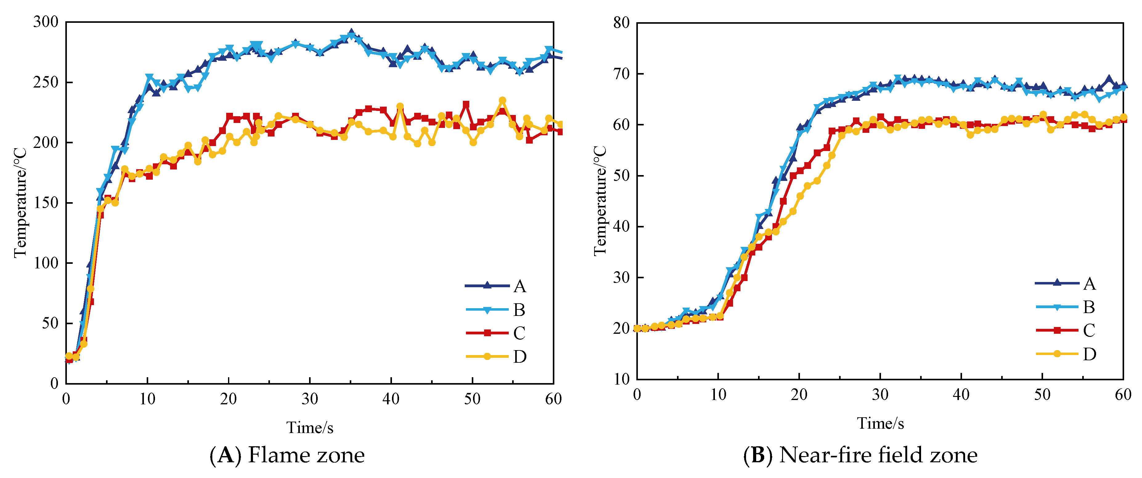
In the fire simulation process, the gridding size is determined by the fire-source characteristic diameter D*. The grid sizes corresponding to the simulated fire-source power in this paper were calculated to be in the range of 0.11–0.45 m. Multiple sets of grids were used to divide the fire field into the flame zone, the near-fire field zone, and the far-from-fire field zone, with different grid sizes, respectively. The square area 5 m away from the fire source is the flame zone, the square area of 10 m is the near fire zone, and up to the boundary is the far fire zone. In order to further verify the accuracy of the simulation calculations, different grid setting scenarios were tested independently, and the four grid setting schemes tested are shown in

Table 2. Grid setup programme.

Grid Programme	Flame Zone (m × m × m)	Near-Fire Field Zone (m × m × m)	Far-from-Fire Field Zone (m × m × m)	Simulation Time
A	0.2 × 0.2 × 0.2	0.25 × 0.25 × 0.25	0.3 × 0.3 × 0.3	53.2 h
B	0.25 × 0.25 × 0.25	0.3 × 0.3 × 0.3	0.4 × 0.4 × 0.4	24.6 h
C	0.35 × 0.35 × 0.35	0.4 × 0.4 × 0.4	0.45 × 0.45 × 0.45	8.7 h
D	0.45 × 0.45 × 0.45	0.45 × 0.45 × 0.45	0.45 × 0.45 × 0.45	5.2 h

.

Figure 8 shows that the temperature fluctuations of C, D are large, and the trends and fluctuations are very inconsistent, especially in the near-fire region, indicating that grids C, D are relatively coarse. Grids A, B overall look not very different, and the temperature change trend and fluctuations have strong consistency, which indicates that the two grid size simulation results are almost the same, and the computation time for A is more than 28.6 h, net B in the accuracy and efficiency of a good compromise between the effect. In addition, in this case it is no longer meaningful to perform a finer meshing than A, and it would be more computationally burdensome. Therefore, we choose the current scheme of mesh B to ensure a balance between the accuracy of the simulation and the feasibility of the simulation time. That is, 0.4 m × 0.4 m × 0.4 m for the far-from-fire field zone, 0.3 m × 0.3 m × 0.3 m for the near-fire field zone, and 0.25 m × 0.25 m × 0.25 m for the flame zone.

2.2.3. Setup for Temperature Prediction

The commercial building has five floors, and the layout of the floors is basically the same except for the ground floor. The third floor was chosen as the experimental site, and a coordinate system was established with the lower-left corner as the origin, the horizontal as the X-axis, and the vertical as the Y-axis, and the sensors were uniformly distributed on the ceiling at a spacing of 5 m, thus establishing 160 measurement points (including temperature, smoke, and CO concentration). As an example, the centre point of the single-floor fire source was located at (13, 15), the size of the fire source was 1 m × 1 m, and two-dimensional temperature slices were created in the vertical and horizontal directions at the centre of the fire source. The distribution of the sensors is shown in Figure 9.

The experimental setup allows the sensors to collect temperature sequence data during fire simulation by setting spatial coordinates (X, Y) for each sensor with X-axis interval [0, 75] and Y-axis interval [0, 50]. Under the same spatial and temporal conditions, there is a strong correlation between different fire environment parameters. In order to create comprehensive and rich training samples, this paper builds a dataset with temperature, smoke concentration, and CO concentration as common inputs to predict the in-plane fire location, and the output is assigned as the coordinates (X, Y) where the fire is located. The sensor acquisition step takes about 1 s, and 300 sets of training samples were obtained for each experiment. A total of six experiments were conducted, totalling 1800 sets of experimental samples. The data samples were used as the input part of the model, and the fire-source coordinates of the six experiments constitute the labelled values as the output part of the model. Then all the labelled samples were randomly divided into training and test datasets with a ratio of 7:3. The training dataset was used to train the model during training, and the test dataset was used to evaluate the quality of the fitted model after training.

3. Research on Fire-Source Location Prediction Modelling

3.1. Hybrid Model Construction

Convolutional Neural Network—Support Vector Machine

The main principle of the support vector machine (SVM) is to find an optimal hyperplane that minimises the error and maximises the distance to the samples in the dataset.

The hyperplane equation is shown in Formula (5).

$$w^{T}x+b=0$$

(5)

where $x$ is the training dataset, $w$ is the separating hyperplane weight vector, $b$ is the bias parameter, and the superscript T indicates a transpose. For the problem that the optimal solution cannot be found for the training set, which is linearly indivisible in the feature space, the objective function can be defined as Formula (6) by introducing the slack variable $\xi$.

$${\min }_{\omega ,\xi }={\displaystyle \frac{{‖w‖}^2}{2}}+C{\displaystyle {\sum }_{i=1}^n{\xi }_i}$$

(6)

introducing the Lagrangian function and selecting the RBF function $K\left(x_i,x\right)$ with better performance. The final regression model is shown in Formula (7).

$$f\left(x\right)={\displaystyle {\sum }_{i=1}^n\left({\alpha }_i-{\alpha }_i^{*}\right)K\left(x_i,x\right)+b}$$

(7)

where ${\alpha }_{*}$ is the Lagrange multiplier introduced in solving the function.

A convolutional neural network (CNN) is a type of feed-forward neural network with excellent local feature extraction capabilities. It usually comprises five layers: input, convolutional, pooling, fully connected, and output. The convolution process can be stated as Formula (8).

$$O=f\left(X\otimes W_C+b_c\right)$$

(8)

where $O$ is the output of the convolutional layer, $W_c$ is the weight matrix, $b_c$ is the bias, $\otimes$ is the convolutional operator, and $f\left(~\right)$ is the activation function.

The activation layer consists of an activation function. The activation function used in this paper is the ReLU function, as shown in Formula (9).

$$f\left(x\right)=\left\{\begin{array}{l}x\left(x>0\right)\\ 0\left(x\le 0\right)\end{array}\right.$$

(9)

The purpose of the pooling layer, sometimes referred to as the down-sampling layer, is to compress the feature map through down sampling and lower the number of neural network parameters. The present investigation employs maximum pooling in conjunction with batch normalisation and the addition of a dropout layer to enhance the model’s convergence speed and generalisability while mitigating the risk of overfitting.

The structure of CNN-SVM is shown in Figure 10.

(a)

After cleaning, modifying the size of the collecting step, and isometric segmentation, the original database is obtained with a training set to test set ratio of 7:3.

(b)

The convolution kernel of Conv_1 and Conv_2 is 3*1 and the step size is 1. Conv_1 has 16 channels, and it produces 16 feature map outputs. Conv_2 has 32 channels, and it produces 32 feature map outputs. Both convolutional layers’ outputs are batch normalised to speed up training, and negative values are set to zero by the ReLU layer.

(c)

To prevent overfitting, the dropout layer discards some neurons as it goes along with a probability of 0.5. The fully connected layer’s output features are then passed to the SVM to get the desired results.

3.2. Crested Porcupine Optimizer

The Crested Porcupine Optimizer (CPO) is a new meta-heuristic algorithm suggested in 2024 to solve optimisation troubles. The program is inspired by the natural behaviour of crown porcupines when seeking food, simulating the four defence strategies they employ when facing predators at varied distances. It also suggests a novel strategy termed cyclic population reduction (CPR) to conserve population variety while accelerating the rate of convergence.

• Cyclic population reduction technique

The strategy simulates the activation of defence mechanisms only when an individual is in danger. During the optimisation process, convergence is accelerated by gradually decreasing the population size. When the population size falls below a certain value, it is gradually increased to improve population variety. This cycle is repeated until the predetermined maximum number of iterations has been met. The process is represented by Formula (10).

$$N=N_{\min }+\left(N^{\prime }-N_{\min }\right)\times \left(1-\left({\displaystyle \frac{t\%\frac{T_{\max }}{T}}{\frac{T_{\max }}{T}}}\right)\right)$$

(10)

where $T$ is the variable that determines the number of cycles, $t$ is the current function evaluation, $T_{\max }$ is the maximum number of function evaluations, and $N_{\min }$ is the minimum number of individuals in the newly generated population.

2.

Crested Porcupine Optimizer

The algorithm first initialises the population, and the process is shown in Formula (11).

$$\overrightarrow{X_i}=\overrightarrow{L}+\overrightarrow{r}\times \left(\overrightarrow{U}-\overrightarrow{L}\right)$$

(11)

where $i=1,2,\dots ,N$; $r$ is a random number. The population obtained after initialising $N$ individuals in the population according to the above formula is shown in Formula (12).

$$X=\left[\begin{array}{l}{X}_1\\ X_2\\ \dots \\ X_i\\ \dots \\ X_N\end{array}\right]=\left[\begin{array}{cccccc}{x}_{1,1}& x_{1,2}& \dots & x_{1,j}& \dots & x_{1,d}\\ x_{2,1}& x_{2,2}& \dots & x_{2,j}& \dots & x_{2,d}\\ \dots & \dots & \dots & \dots & \dots & \dots \\ x_{i,2}& x_{i,2}& \dots & x_{i,j}& \dots & x_{i,d}\\ \dots & \dots & \dots & \dots & \dots & \dots \\ x_{N,1}& x_{N,2}& \dots & x_{N,j}& \dots & x_{N,d}\end{array}\right]$$

(12)

(a)

The first defence strategy is as in Formula (13).

$$\left\{\begin{array}{l}\overrightarrow{x_i^{t+1}}=\overrightarrow{x_i^t}+{\tau }_1\times \left|2\times {\tau }_2\times \overrightarrow{x_{cp}^t}-\overrightarrow{y_i^t}\right|\\ \overrightarrow{y_i^t}={\displaystyle \frac{\overrightarrow{x_i^t}+\overrightarrow{x_r^t}}{2}}\end{array}\right.$$

(13)

where $\overrightarrow{x_i^{t+1}}$ is the position of the individual at the next iteration, ${\tau }_1$ is a random number that obeys a normal distribution, ${\tau }_2$ is a random number that lies in the interval from 0 to 1, $x_{cp}^t$ is the current global optimal solution, $y_i^t$ represents the position of the predator, and $r$ is a random number between $[1,N]$.

(b)

The second defence strategy is shown in Formula (14).

The approaching or moving away of a predator is used to prevent the population from concentrating too much on the current optimal solution, thus avoiding falling into a local optimum when the predator approaches. The second defence strategy is executed.

$$\overrightarrow{x_i^{t+1}}=\left(1-\overrightarrow{U_1}\right)\times \overrightarrow{x_i^t}+\overrightarrow{U_1}\times \left|\overrightarrow{y}+{\tau }_3\times \left(\overrightarrow{x_{r1}^t}-\overrightarrow{x_{r2}^t}\right)\right|$$

(14)

(c)

The third defence strategy is as in Formula (15).

$$\overrightarrow{x_i^{t+1}}=\left(1-\overrightarrow{U_1}\right)\times \overrightarrow{x_i^t}+\overrightarrow{U_1}\times \left(\overrightarrow{x_{r1}^t}+S_i^t\times \left(\overrightarrow{x_{r2}^t}-\overrightarrow{x_{r3}^t}\right)-{\tau }_3\times \overrightarrow{\delta }\times {\gamma }_t\times S_i^t\right)$$

(15)

where $r_3$ is a random number located between $[1,N]$, ${\tau }_3$ is a random number located between $[1,N]$, $\delta$ is a parameter controlling the search direction, ${\gamma }_t$ is a defence factor, and $S_i^t$ is an odour diffusion factor. The solution formula is Formula (16).

$$\left\{\begin{array}{l}\overrightarrow{\delta }=\left\{\begin{array}{l}+1,if \overrightarrow{rand}\le 0.5\\ -1,else\end{array}\right.\\ {\gamma }_t=2\times rand\times {\left(1-{\displaystyle \frac{t}{t_{\max }}}\right)}^{{\displaystyle \frac{t}{t_{\max }}}}\\ S_t^i=\exp \left({\displaystyle \frac{f\left(x_t^i\right)}{{\displaystyle {\sum }_{K=1}^{N}f\left(x_t^K\right)+\in }}}\right)\end{array}\right.$$

(16)

(d)

The fourth defence strategy is as in Formula (17)

When the predator is close, the CP will attack it with short and thick quills and execute the fourth defence strategy.

$$\left\{\begin{array}{l}\overrightarrow{x_i^{t+1}}=\overrightarrow{x_{cp}^t}+\left(\alpha \left(1-{\tau }_4\right)+{\tau }_4\right)\times \left(\delta \times \overrightarrow{x_{cp}^t}-\overrightarrow{x_i^t}\right)-{\tau }_5\times \delta \times {\gamma }_t\times \overrightarrow{F_i^t}\\ \overrightarrow{F_i^t}=\overrightarrow{{\tau }_6}\times m_i\times \left(\overrightarrow{v_i^{t+1}}-\overrightarrow{v_i^t}\right)\end{array}\right.$$

(17)

where $\alpha$ is the velocity convergence factor, ${\tau }_4$ is a random number located between, $F_i^t$ is the inelastic collision force generated when an individual attacks a predator with its body, and $\overrightarrow{{\tau }_6}$ is a random vector between $[0,1]$.

3.

Execution steps

Step 1: Initialise the parameters according to Formula (11). Set the population size $\left(N\right)$, the maximum number of iterations $\left(T\right)$, the dimensions of the solution $\left(\dim \right)$, the lower boundary of the solution space $(L)$, and the solution space’s upper boundary $(U)$, and after completing the initialisation, the individual with the highest fitness is chosen as the current global optimal solution.

Step 2: The population begins searching the solution space and updates each individual position. By comparing the sizes of two generated random numbers, ${\tau }_8,{\tau }_9$, determine whether to perform a global search or local exploitation.

Step 3: When ${\tau }_8<{\tau }_9$, perform the global search, and vice versa perform local exploitation. The global search contains two methods, which can be determined by comparing the size of two generated random numbers ${\tau }_6$ and ${\tau }_7$ to determine whether to perform the first defence strategy or the second defence strategy.

Step 4: When ${\tau }_6<{\tau }_7$, execute the first defence strategy, which is the mathematical model as Formula (13). Conversely, the second defence strategy is executed, which is the mathematical model as Formula (14).

Step 5: When ${\tau }_8>{\tau }_9$, execute local exploration, which can be determined by comparing the sizes of two generated random numbers ${\tau }_{10}$ and $T_f$. The rationale is the same as the global exploration stage.

Step 6: When ${\tau }_{10}<T_f$, execute the third defence strategy, which is the mathematical model as Formula (16). Conversely, the fourth defence strategy is executed, which is the mathematical model as Formula (17).

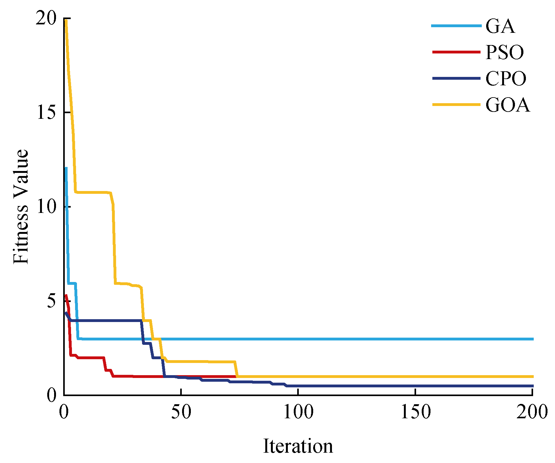
3.3. Algorithm Performance Comparison

In order to verify the effectiveness of the optimisation of the CPO algorithm, we compared it with the PSO, GA, and GOA algorithms. In the CPO algorithm, the number of population n = 120, the number of loops t = 2, the convergence rate alpha = 0.2, the trade-off percentage between the third and the fourth defence mechanism T_f = 0.8, the inertia weights inertia = 0.9, and c1 = c2 = 2. The PSO algorithm adopts a linearly decreasing inertia weight strategy, with the initial weight 0.9 gradually decreasing to 0.6. The GA algorithm has a crossover probability of 0.8 and a variance probability of 0.15. The GOA algorithm has coefficients c in the range of [0.00004, 1], with coefficient constants f = 0.5 and l = 1.5. Figure 11 shows a comparison of the algorithms, optimising the hyperparameters of the CNN-SVM model for location prediction. PSO and GA converge quickly and easily fall into local optimisation, GOA fluctuates greatly and is less stable, and CPO converges smoothly and finally reaches the lowest objective function value, showing good robustness. The final CNN-SVM model key parameters of optimal learning rate, hidden layer nodes, and regularisation coefficients take the optimal values of 0.0042, 28, and 0.0001, respectively.

3.4. CPO-CNN-SVM

The hybrid model CPO-CNN-SVM’s prediction process is divided into three modules: data input, training input, and result output, as shown in Figure 12.

After establishing the fire field dataset, the data is divided into training and testing sets, containing key factors such as temperature field and spatial distribution at different time periods after the fire. After initialising the parameters of the CPO algorithm, the CNN-SVM model is begun to be trained. The model optimises the parameters to seek the global optimal solution in each iteration round based on updating the fitness values of the individuals, and it continuously makes a judgment on whether the set maximum number of iterations has been reached. In the training input, the CNN model firstly performs parameter initialisation to extract the spatiotemporal features of the fire data; then, these features go through the convolutional layer, pooling layer, and fully connected layer, and are finally used as inputs to train the SVM model, forming the fusion model CNN-SVM.

To improve the performance of the fusion model CNN-SVM, the CPO algorithm is used to optimise the key hyperparameters of the CNN-SVM model, including the learning rate, the number of nodes in the hidden layer, and the regularisation factor. The optimised CPO-CNN-SVM model can effectively improve the accuracy of fire field prediction. The model learns the spatiotemporal evolution laws in this data through training to achieve accurate prediction of the fire field, and SVM is used as an output module to achieve real-time prediction of the temperature field and determination of the fire-source location. The convolutional, pooling, and fully connected layer structure of the CNN can efficiently capture spatial and temporal features in the dynamic evolution of the fire, and it can extract spatiotemporal information from a large amount of data, providing high-quality inputs for the SVM model. The CPO-CNN-SVM model outputs the coordinates of the predicted fire location. Based on the prediction results, decision-makers can take timely emergency measures to reduce the losses caused by fire.

In the hybrid model prediction process, model optimisation is a dynamic and continuous process. After the model generates preliminary prediction results, the system adjusts the parameters of the CPO algorithm through a feedback mechanism according to the deviation of the prediction results from the actual situation to further optimise the model. Each round of training is based on the updated data, and the accuracy of the prediction is gradually improved to achieve high-precision fire field prediction.

Overall, CNN can extract temporal and spatial features from a large amount of fire scene data, extract features from within a local area through operations such as convolution and pooling, and retain the spatial structure information of the features as the input to SVM, whose kernel function can map the features into a high-dimensional space to better portray the nonlinear relationships among the features. The CPO algorithm avoids ineffective or unnecessary parameter spatial searches by enhancing the model’s understanding of the relationships between the data, thus improving overall performance.

4. Results

4.1. Analysis of Fire-Source Location Results

Twelve sets of experiments were set up in the building plan, with fire centre coordinates of (17, 8), (20, 12), (25, 35), (32, 19), (40, 24), (11.5, 4), (7.5, 15.8), (54.3, 40.6), (60.7, 43.9), (67.5, 47.4), (72.1, 50), and (47, 29); these locations constructed a localisation inversion prediction based on fire-source parameters. Similarly, 12 fire scenarios were generated through FDS simulation. The output was assigned coordinate value labels, the model learned through a training set, and the test set evaluated the goodness of fit of the model’s fire-source coordinates.

To assess the validity of different models, this paper used the root mean square error (RMSE), mean absolute percentage error (MAPE), mean absolute error (MAE), and coefficient of determination R².

$$RMSE=\sqrt{{\displaystyle \frac{1}{n}}{{\displaystyle {\sum }_{i=1}^n\left(y_i-{\widehat{y}}_i\right)}}^2}$$

(18)

$$MAPE={\displaystyle \frac{1}{n}}{\displaystyle {\sum }_{i=1}^n\left|\frac{y_i-{\widehat{y}}_i}{y_i}\right|\times 100\%}$$

(19)

$$MAE={\displaystyle \frac{1}{n}}{\displaystyle {\sum }_{i=1}^n\left|y_i-{\widehat{y}}_i\right|}$$

(20)

$$R^2=1-{\displaystyle \frac{{\displaystyle {\sum }_{i=1}^n{\left(y_i-{\widehat{y}}_i\right)}^2}}{{\displaystyle {\sum }_{i=1}^n{\left(y_i-\overline{y}\right)}^2}}}$$

(21)

where $y_i$ is the actual value of the collected temperature data, ${\widehat{y}}_i$ is the predicted value of the network output, $\overline{y}$ is the average of the actual value of the temperature, and $R^2$ represents the model’s goodness of fit; the closer it approaches 1, the better the fit.

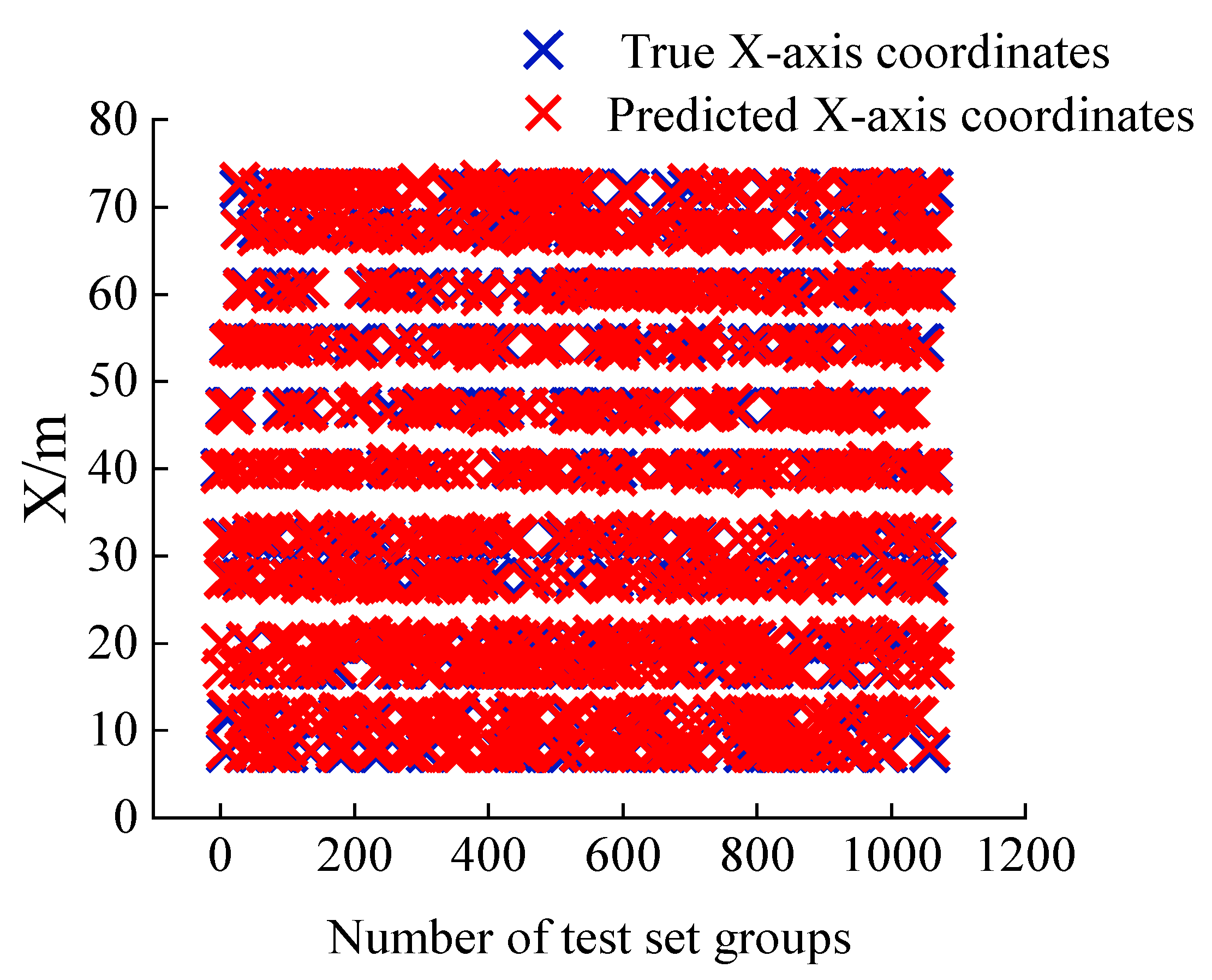
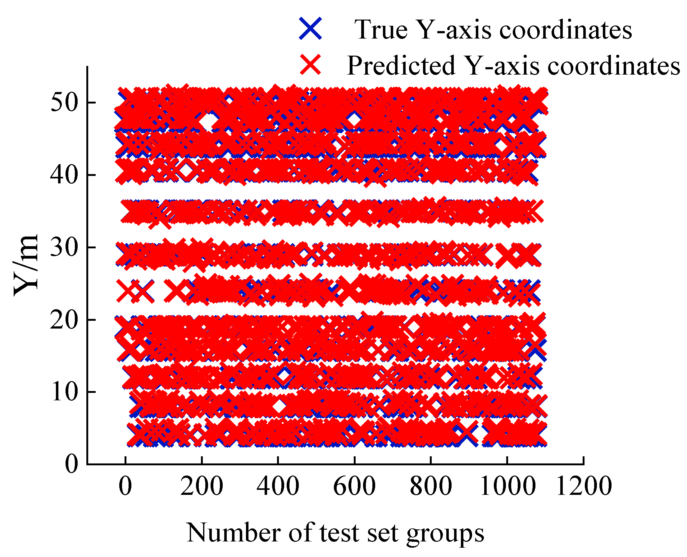
The model X, Y coordinate prediction results for the test set are shown in Figure 13 and Figure 14, respectively. It can be seen that the distribution of the predicted points coincides with the labels, and only a small number of points deviate, indicating that the model performs well in the spatial coordinate prediction task. The X-axis coordinate R² is 0.99, the Y-axis coordinate R² is 0.99, the X-axis coordinate MAPE is 1.56%, the Y-axis coordinate MAPE is 1.67%, the maximal absolute error of the X-axis coordinate is 0.97 m, and the maximal absolute error of the Y-axis coordinate is 0.96 m.

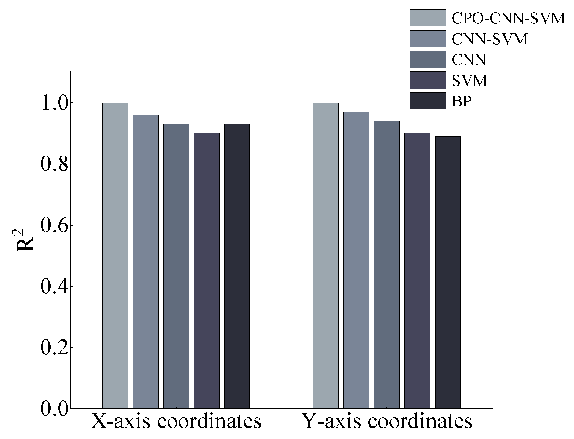
Figure 15 shows the comparative analysis of the model R² values, indicating that the CPO-CNN-SVM model demonstrates a significant advantage in the task of fire-source coordinate prediction. The X-axis and Y-axis test set R² of the CPO-CNN-SVM model is 0.99, which is much higher than the other comparative models (CNN-SVM, CNN, BP, and SVM), whose R² values are generally lower than 0.97. The CPO-CNN-SVM model effectively captures spatial features (e.g., temperature, smoke, and CO concentration) in the fire data via a convolutional neural network (CNN). In contrast, the traditional BP neural network with a single SVM model finds it difficult to parse the multi-scale correlations of a complex fire scenario due to the lack of feature hierarchical extraction capability. Although CNNs can automatically extract spatial features through convolutional layers, they usually use fully connected layers at the end for regression prediction. The linear combination property of fully connected layers may lead to sensitivity to outliers. The introduction of the CPO algorithm enhances the adaptive adjustment of model parameters, avoids the local optimum problem and unnecessary solution space search caused by manual parameter tuning in traditional models (e.g., SVM, BP), and improves the model’s generalisability to nonlinear fire dynamics. It provides a reliable technical path for the real-time localisation of commercial building fires, based on which the model’s adaptability in extreme scenarios involving noise interference and sensor failure can be further explored to promote practical engineering applications.

Table 3. Model Error Indicators.

Model	Coordinate Axis	Error Indicator
		MAE	RMSE
CPO-CNN-SVM	X	0.35	0.41
	Y	0.26	0.38
CNN-SVM	X	0.62	2.31
	Y	1.23	2.65
CNN	X	0.89	2.01
	Y	0.95	2.18
BP	X	2.56	3.77
	Y	2.43	3.26
SVM	X	1.89	3.24
	Y	1.58	2.87

shows the comparison of model fire location error metrics. It can be seen that the CPO-CNN-SVM model shows significant superiority in the fire-source location prediction task. In the X-axis direction, the MAE and RMSE of the model are 0.26 and 0.39, respectively, and in the Y-axis direction, the errors are reduced to 0.20 and 0.31, which are both significantly better than the comparison model. The MAE of the CNN-SVM model without the introduction of the CPO module in the X-axis and Y-axis rises to 0.62 and 1.23, respectively; the RMSE is 2.31 and 2.65, respectively; and the longitudinal positioning is unstable, indicating that the CPO module plays a key role in improving the spatial positioning accuracy of the model. The traditional BP neural network and SVM model have larger errors, with the RMSE of the BP model in both the X-axis and Y-axis directions being more than 3.1, and the accuracy of the SVM model being higher as well. In summary, the CPO-CNN-SVM model effectively integrates spatial feature extraction and the nonlinear mapping mechanism to achieve high-precision prediction of the fire-source location, demonstrating good robustness and practical application value.

4.2. Analysis of Fire-Source Room Localisation Results

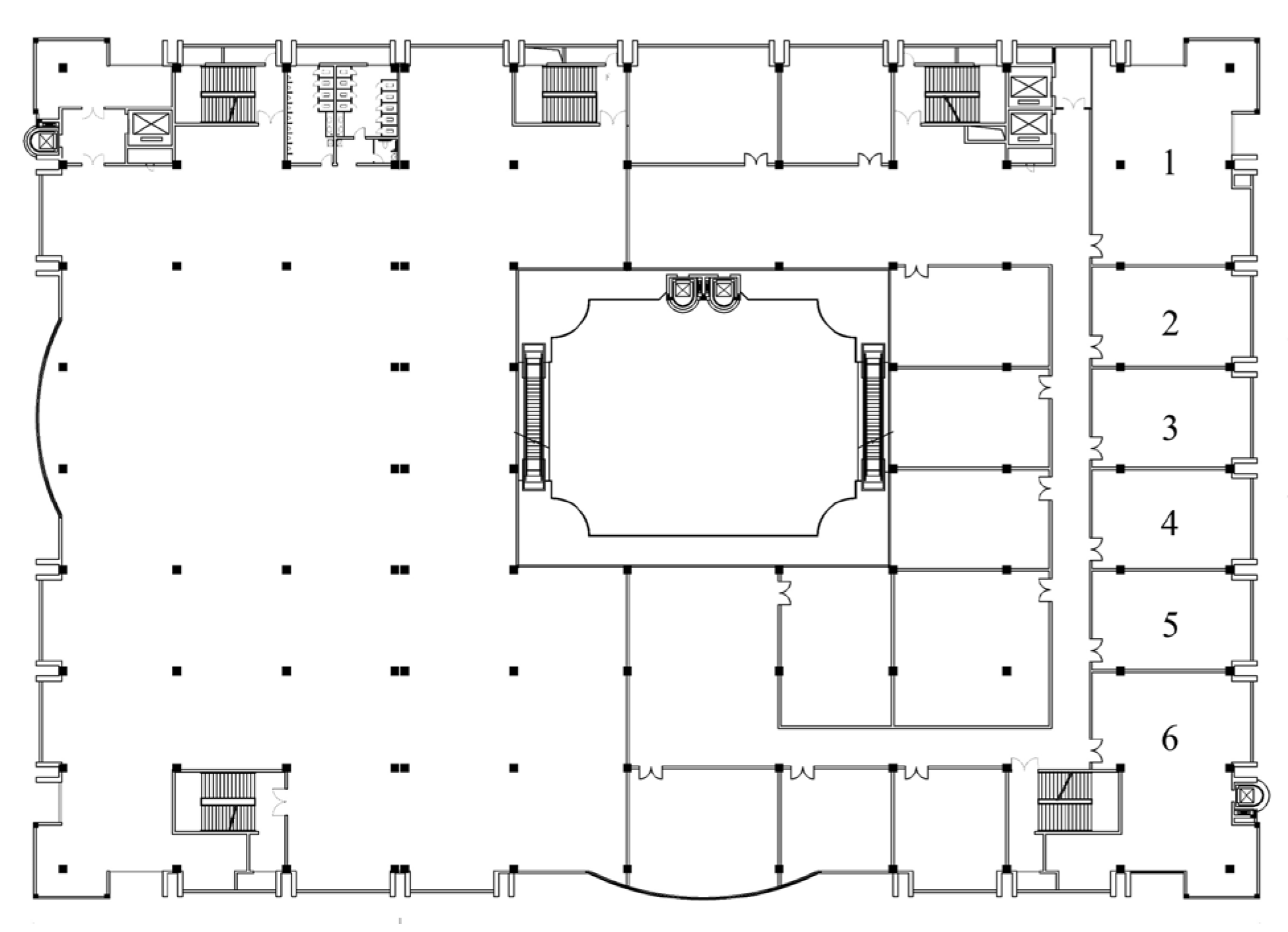
In order to further enhance the model application scenarios, experiments for localisation at the compartment (room) level where the fire source is located were conducted. The fire was simulated to occur in a functional room of the identified fire-source floor to establish the experimental scenario. The above experiments were based on 160 sensors uniformly distributed on the ceiling to establish a training dataset with a large amount of data, considering the influence of the irregular distribution of sensors on the prediction effect of the model. In this experiment, the fire source was set in the centre of six compartments on the west side, and 10 measurement points were set up at three different heights in the corridor (3 m, 4 m, and ceiling) for a total of 30 temperature measurement points to perform a fire simulation of a fire occurring in the centre of the six compartments and to locate the room where the fire was occurring based on the temperature sequence data collected from the 30 measurement points. Figure 16 shows a schematic diagram of the compartments in this layer of the experiment.

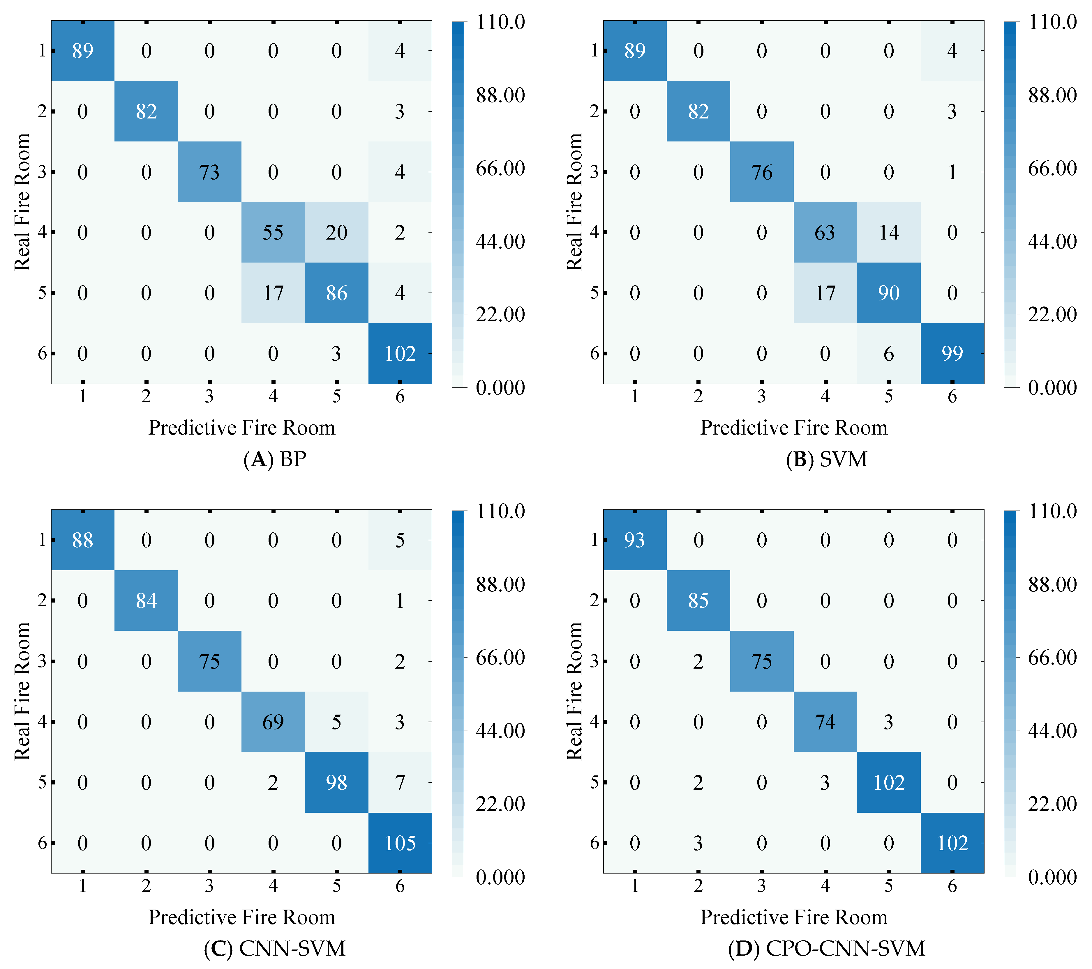
Figure 17 shows the model fire-source room localisation confusion matrix, and Figure 17A–D show the BP, SVM, CNN-SVM, and CPO-CNN-SVM models, respectively. The vertical axis indicates the actual fire-source room, the horizontal axis indicates the predicted fire-source room, and the diagonal line indicates the number of correctly predicted samples; the closer to the complete diagonal distribution, the higher the model localisation accuracy. As a whole, all models achieved high accuracy in most rooms, especially rooms 1, 2, and 6, but there was confusion in the identification of rooms 4 and 5, with room 4 predicted as room 5 in all model tests; SVM and BP performed especially poorly. By analysing the experimental results and tracing the causes, it was found that this phenomenon is due to the fact that the fire-source occurred in two adjacent rooms with similar size and structure, and as the heat flow of the fire source propagated along the corridor, it was very likely to affect the neighbouring rooms, making the temperature field in the region more similar, causing difficulties and model confusion. The CPO-CNN-SVM model performed best and was stable in edge room localisation, with a prediction accuracy of 5 out of 6 rooms exceeding 90%, of which rooms 4, 5 and 6 were the most accurate in terms of discrimination, and with an overall accuracy as high as 97.61%, which maximally overcame the problem of confusing the identification of neighbouring fire-source rooms.

4.3. Analysis of the Model’s Anti-Jamming Performance

By choosing different sensor damage situations and damage rates to simulate complex working conditions, the hybrid model CPO-CNN-SVM was used to conduct prediction experiments to test the anti-interference performance of the model in complex situations. The effects of different damage locations (distance from the fire source) and different damage degrees (damage rate from low to high) on the model prediction performance are discussed for a total of 126 working conditions.

(1)

Effect of different sensor damage rates on the model

In order to avoid the subjective judgement of manual selection and at the same time to ensure the reproducibility of the experiments, the sensor damage process was implemented by randomly generating damage points through the code to ensure that the damage configurations of the training set and test set generated from each experiment had the same conditions. The sensor network was first created with sensors spaced at 5 m. Damage ranged from 10% to 70% with a 10% damage gradient. Damaged sensor indexes (damaged_idx) and damage rate (damage_ratio) records were constructed through the code. In addition, in order to facilitate subsequent analysis, the damage dataset created not only included normal sensor data (clean_data) but also recorded the location information of damaged sensors (sensor_coords). Through this sensor damage simulation method, multiple working conditions with different sensor damage rates could be established to validate the model, analyse in-depth the interference resistance of the CPO-CNN-SVM model under different sensor damage conditions, and assess the robustness and reliability of the model in complex environments. Figure 18 shows an example of a 20% damage rate for a sensor with an ignition source at (25, 35). Seven different sensor damage scenarios, 6 ignition source locations, and a total of 42 working conditions. Experiments were carried out for each fire location with 7 different sensor damage rates to verify the validity of the model.

(2)

Effect of different sensor damage locations on the model

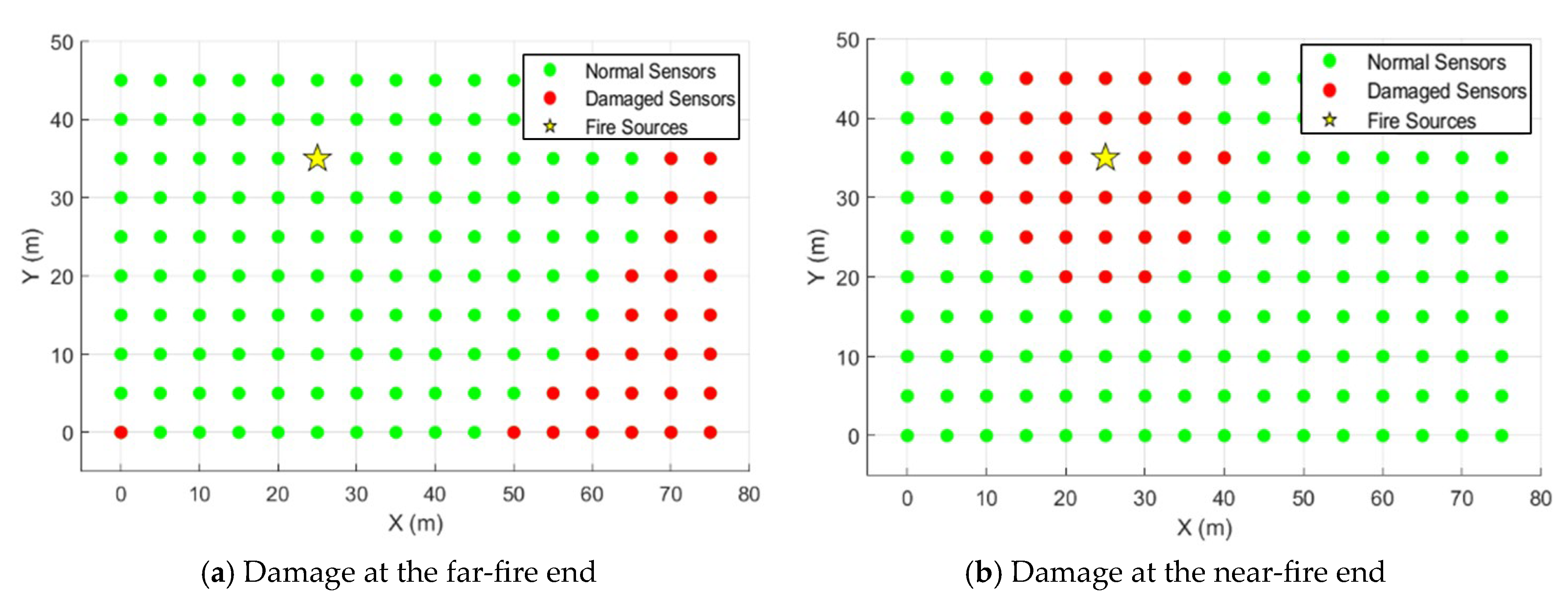
To further assess the performance of the model comprehensively, the impact of different damage locations of the sensor on the predictive performance of the model was further analysed based on random damage to the sensor. Figure 19 shows the schematic diagram when the extreme damage rate is 20%, including two scenarios: Figure 19a, damage at the far-fire end, and Figure 19b, damage at the near-fire end. The damage rate is graded from 10% incrementally to 70%, with seven damage scenarios, resulting in a total of 84 working conditions for the experiment. Using normal data to train the model, the model predicted the missing values by learning the mapping relationship between other sensors and the target sensor when the sensor was damaged, using the real-time data from other sensors to input the model, and, theoretically, the usual positive correlation between the prediction deviation and the damage rate.

Figure 20 shows the average deviation of model position prediction with damage rate for 42 working conditions involving random sensor damage and 84 working conditions with different sensor damage locations and damage rates. It can be seen that the accuracy of prediction is closely related to the location of the sensor damage. The data of the near-fire source changes drastically and critically. All the sensor damage here has the greatest impact on the prediction results, with the error in the critical area accumulating, and the average position deviation reaching 17 m. While the temperature rise at the far-fire-source end is gentle, the temperature difference between the target sensor and the surrounding sensors is not large, and the model can compensate for the damage by using data from other sensors with better learning, so the damage impact is smaller. Whereas random damage generally does not result in an extreme situation of a large area of missing data or an anomalous region, the model can fully learn the temperature data of the neighbouring points for prediction, and the position prediction deviation is minimal.

(3)

Analysis of modelled fire-source room localisation with small sample data

We designed a total of three different damage scenarios to verify the anti-jamming performance of the model on a small sample dataset. The damage cases included sensor interval damage, centralised damage to one end sensor, and centralised damage to two end sensors. The above experimental damage rates are uniform intervals, so this time, different intervals were selected for experiments to enrich the testing conditions of the model and verify its generalisation performance. The damage rate was taken as 20%, 40%, 60%, 70%, 75%, and 80% in six damage cases, for a total of 18 conditions for fire-source room localisation verification experiments.

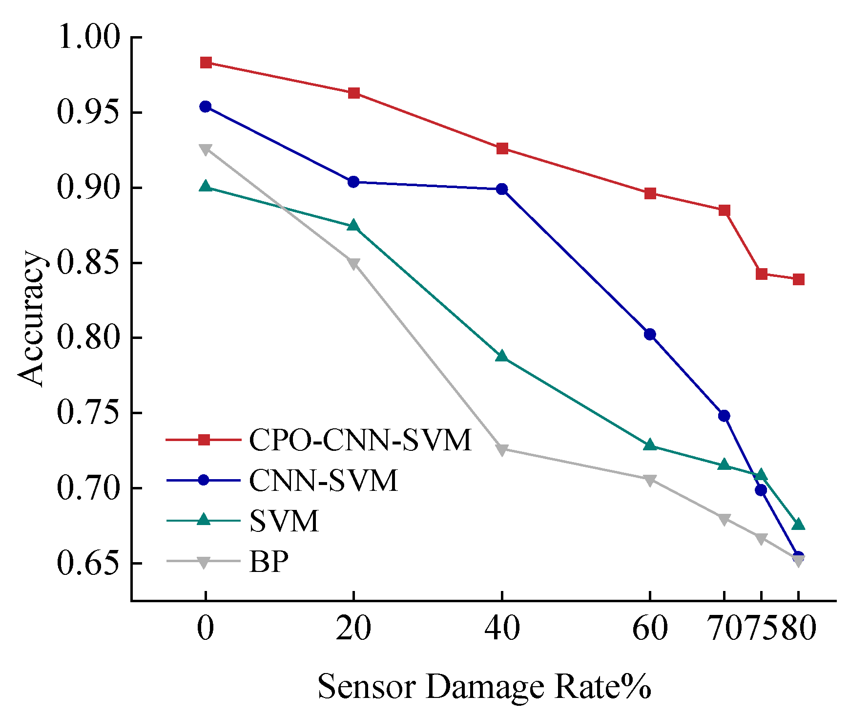
Figure 21 shows the variation of fire location prediction accuracy of each model under sensor interval damage. As the sensor damage rate increases, the accuracies of all the models decrease, but the magnitude of the decrease varies. The CPO-CNN-SVM model shows the strongest stability under this condition, and the accuracy remains above 92% even when the sensor damage rate reaches 80%. In contrast, the CNN-SVM model can adapt to sensor damage to some extent and outperforms the traditional SVM and BP models in terms of performance, but the decrease in accuracy is still more obvious. The SVM and BP models found it difficult to maintain high accuracy in this case; especially after the damage rate exceeded 40%, the accuracy rate dropped significantly. Therefore, the CPO-CNN-SVM model has good robustness and can effectively deal with the problem of missing data.

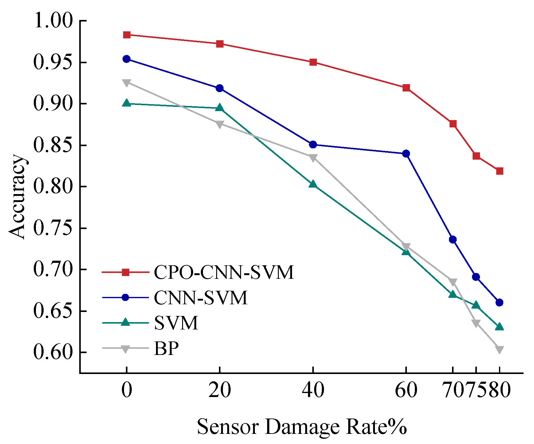
Based on the analysis of the impact of sensor damage rate on prediction accuracy, the factor of the location of the sensor damage was further taken into account. Since the measurement points in this scenario are symmetrically distributed, the impact on prediction accuracy is similar when the sensors are damaged centrally at the upper and lower ends of the corridor. Therefore, this paper selects the two scenarios of sensor damage concentrated at the upper end of the corridor and the two ends of the corridor to be analysed, as shown in Figure 22 and Figure 23.

It can be seen that, compared with the sensor interval damage case, these two concentrated damage cases have a greater impact on the models, and the prediction accuracies of all the models show decreasing trends of different degrees. However, the CPO-CNN-SVM model still shows strong anti-interference ability in the face of these two extreme damage cases. When the damage rate reaches 80%, the accuracy of the model can still be maintained above 80%. If the prediction accuracy of the CPO-CNN-SVM model is kept above 90%, the damage rate should be controlled within 40% when the sensors are concentrated at the same end. When the sensors are concentrated at both ends of the channel, the damage rate should be controlled at 60%. When the damage rate is 70%, the prediction accuracies of the CPO-CNN-SVM model in these two cases are 88.5% and 87.61%, respectively, which are significantly better than other models. In contrast, when the damage rate exceeds 60%, the accuracy of CNN-SVM begins to decline significantly. When the damage rate exceeds 20%, the accuracies of SVM and BP decline significantly. In summary, the concentrated damage of edge sensors to the model can cause a significant decline in model prediction accuracy. Therefore, the regular inspection of sensors in buildings should be strengthened to ensure the reliability of the system and prevent the adverse effects of high-concentration damage rates.

4.4. K-Fold Cross Validation

After identifying the CPO-CNN-SVM model as the most effective model for location prediction work, its performance was verified using K-fold cross-validation. K-fold cross-validation is a method commonly used to test the generalisation performance of machine-learning models. The main idea is that by dividing the dataset into K subsets of the same size, the model can be trained and validated on each subset (the model is trained on K − 1 subsets, then the last subset is tested), and the process is repeated several times. In each repetition, the model learns the intrinsic laws and features of the data by effectively using the limited dataset for training and accurately evaluates the performance of the model on unknown data.

The steps of K-fold cross-validation are as follows:

Step 1: Assuming that the original data contains N samples, K-fold crossover will divide the dataset into K subsets, each of which has a size of about ${\displaystyle \frac{N}{K}}$.

Step 2: Each time, a subset is selected as the validation set, and the other K−1 subsets are used as the training set, which trains the model and calculates the evaluation metrics for that round.

Step 3: The process is repeated K times, and each time a different subset is selected as the validation set, so each subset is selected once for validation and the others as the training set.

Step 4: The final performance evaluation takes the average of the K-fold cross-validation results, which can be used to assess the generalisation performance of the model.

K generally takes the value range between [2, 10], and in this paper, we chose K = 2, K = 5, and K = 10 to observe the error index of the model and take the temperature field prediction as an example to analyse its stability and generalisation ability.

Table 4. Cross-validation error metrics for different K-folds of the model.

Verification of the Situation	Error Indicator
	R2	RMSE	MAPE%
K = 2	0.88	8.07	6.33
K = 5	0.91	6.81	5.68
K = 10	0.93	6.21	5.60

shows the results of the cross-validation error index of the CPO-CNN-SVM model with different K values.

When K = 2, the model is trained with only 50% of the data, it is easy to underfit, the results are affected by random division, and the index fluctuates greatly; when K = 5, the validation set accounts for 20% and the randomness is reduced by averaging many times, but there may still be local bias; when K = 10, the model is trained with 90% of the data, and it covers more subsets of the data, it learns more adequately, and the evaluation results are closer to the true generalisation performance; it is the best in terms of stability. From K = 2 to K = 5, the model’s R² improves by 0.03, the RMSE decreases by 1.26, and its MAPE decreases by 0.65%. From K = 5 to K = 10, the model’s R² improves by only 0.02, the RMSE decreases by 0.60, and its MAPE decreases by 0.08%.

From the validation results, with the increase of K, the R² of the model gradually increases, the fit of the model gradually improves, the RMSE and MAPE values gradually decrease, and the error gradually decreases, which indicates that when the model uses more samples for training, it can learn the data features better, and its prediction performance is better. If K > 10 is selected for validation, the enhancement effect will be limited, and the computational burden will be increased. To balance the computational efficiency and accuracy, 10-fold cross-validation can be chosen to train the final model in the application to ensure the generalisation performance.

4.5. Analysis of the Contribution of Model Input Features to Localisation Accuracy

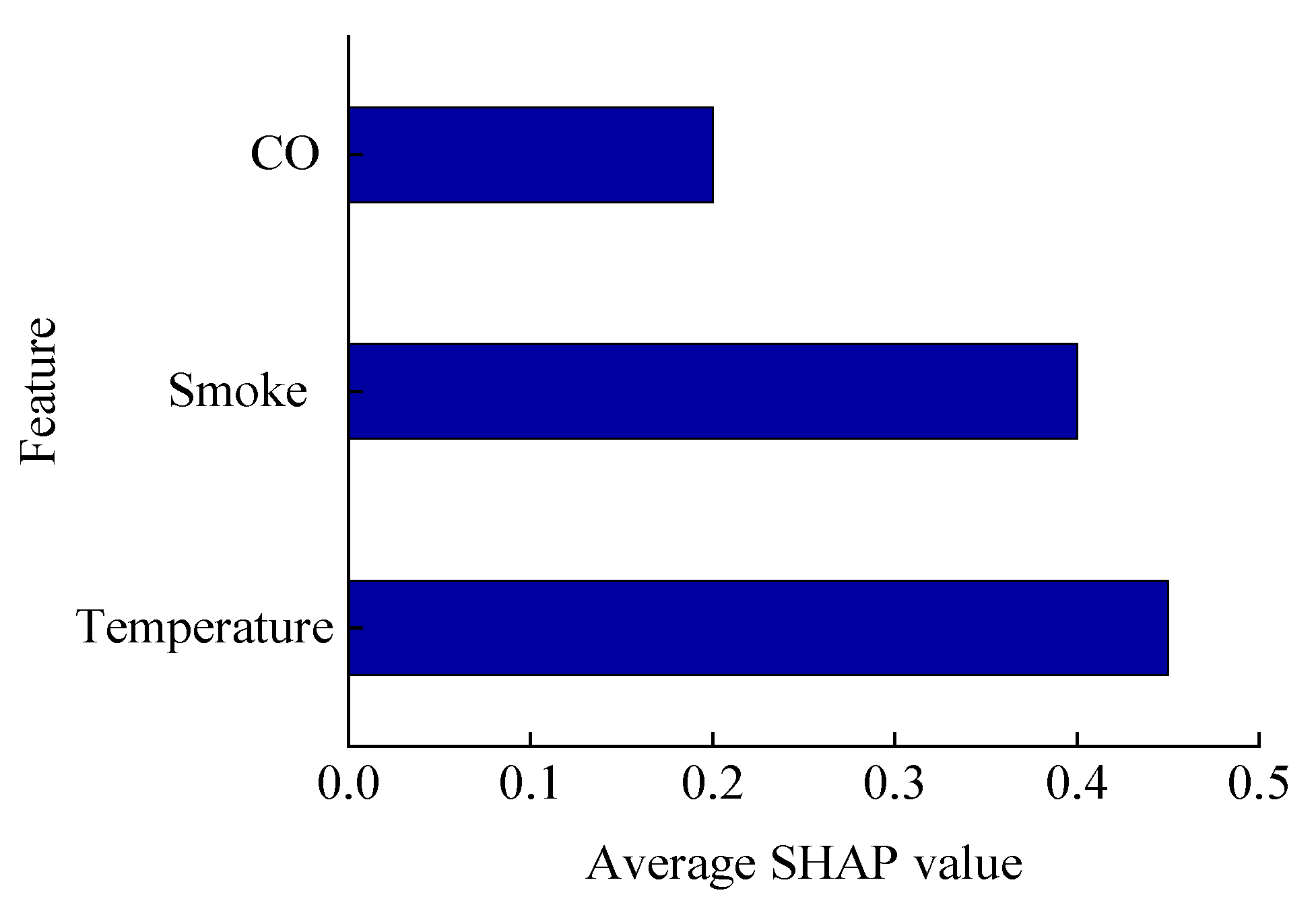
In order to gain a deeper understanding of the model’s dependence on different sensor input features in the fire-source localisation task, this study employs the SHapley Additive exPlanations (SHAP) method to conduct an interpretable analysis of the model’s decision-making process. SHAP is based on the Shapley value theory of game theory, which can quantitatively assess the contribution of each feature in the model output, thus revealing the relative importance of each feature in the forecast. This section analyses the extent to which three key input variables—temperature, smoke concentration, and carbon monoxide (CO) concentration—affect the prediction of fire location.

Figure 24 shows the analysis of SHAP values for the model input variables. The average SHAP values for temperature and smoke are 0.45 and 0.4, respectively, and CO is 0.2. It can be seen that temperature contributes the most to location prediction, with smoke and CO decreasing gradually.

5. Conclusions

In this paper, a commercial building fire numerical model is established with an industrial building as the research object. Combining the fire dynamics simulation with the machine-learning method of the hybrid model, a hybrid model fire-field prediction method based on CPO-CNN-SVM is proposed, which can be used for fire-source location determination. The main conclusions include

(1)

A commercial building fire model was constructed based on FDS using Pyrosim software, and a numerical model of a commercial building fire with multiple scenarios was established to simulate a variety of complex working conditions. In the simulation process, the distribution characteristics of temperature in the dynamic process of fire were fully considered, and three fire zones were divided into different grid schemes according to the spatial distance from the fire source, from near to far, and the best nested grid scheme was selected according to the results of a grid independence test. The approximate accuracy of the numerical simulation was improved under the premise of ensuring computational efficiency. Moreover, the consistency of the single-room fire experimental data was verified to ensure the reliability of the numerical simulation, thus providing high-quality datasets for subsequent model training.

(2)

A hybrid prediction model, CPO-CNN-SVM, was constructed by integrating deep-learning and optimisation algorithms, which significantly improves the accuracy and robustness of fire field prediction compared with the unoptimised model. The hybrid model combines the strong generalisation ability of SVM with the feature extraction advantage of CNN, and at the same time introduces the Crown Porcupine Optimization algorithm (CPO) to jointly optimise the model hyperparameters, thereby enhancing the global search capability of the model performance. The model is not only able to automatically learn the spatiotemporal feature relationship of the temperature field, but it can also accurately complete the data mapping of the high-dimensional feature space and then realise the prediction of the location of the fire source in commercial building fires.

(3)

The model outperforms the unoptimised conventional model on all error assessment metrics for 12 different fire-source location predictions and six fire-source room localisations, with the MAE within 0.35, the RMSE within 0.41, and fire-source room prediction accuracy up to 97.61%. The anti-interference performance of the model was also cross-validated under three sensor damage scenarios, multiple sensor damage rates, and different K values. The results show that the model has certain anti-interference ability and strong generalisation performance.

Finally, this paper demonstrates the versatility of the proposed model by combining a fire dynamics simulator with machine learning for fire-source localisation in commercial buildings, including fire coordinate prediction and fire room localisation. The machine-learning model was trained by generating temperature, smoke, and CO data from the fire dynamics simulation to learn the physical correlation between fire combustion patterns and spatial features for early fire pinpointing. Using the dynamic information provided by this detection system, fire victims and fire rescue personnel can choose the best evacuation and rescue routes to reduce the casualties and property losses caused by fire.