Research on an Intelligent Prediction Method for the Carbon Emissions of Prefabricated Buildings During the Construction Stage, Based on Modular Quantification

Abstract

Prefabricated buildings are widely utilized due to their effectiveness in reducing carbon emissions. The construction stage has a significantly higher carbon emission rate than the other stages of their life cycle, but this is difficult to accurately quantify and predict due to the high variability. This study clarifies the system boundary of carbon emissions and the parameters of influence in carbon emissions predictions. The carbon emission quantification model was improved by using the process analysis method and the carbon emission factor method, and a modular calculation formula was proposed. Based on the machine learning algorithm, a carbon emissions prediction model for prefabricated buildings’ construction stage was established and hyperparameter optimization was conducted. A sample database for predicting prefabricated buildings’ carbon emissions during the construction stage was established using a modular quantification method, and the thin plate spline interpolation algorithm was introduced to expand this. The prediction results of carbon emission prediction models using four algorithms, SVR, BPNN, ELM, and RF, were compared and analyzed by RMSE and R². The results show that the model based on BPNN has the highest prediction accuracy when determining the carbon emissions of prefabricated building during the construction stage, and this method can provide a more accurate reference for subsequent quantitative research on carbon emissions from prefabricated buildings.

1. Introduction

Due to the effects of global warming, various industries promote low-carbon transformation, and the construction industry, as a key area of carbon emissions, has become the focus of carbon emission reduction [1,2]. Prefabricated buildings have technical advantages in terms of waste reduction, etc., and the number new constructions continues to increase, accounting for a larger proportion of new buildings each year [3,4,5,6]. Therefore, the study of prefabricated buildings has great potential to reduce carbon emissions. How to accurately quantify and predict the carbon emissions over the life cycle of prefabricated buildings has also become a hot topic in the research of many scholars [7].

Most of the current research focuses on carbon emissions throughout the building’s entire life cycle, but there is a lack of research on carbon emission reduction during the construction stage [8]. Compared with other stages, the construction stage involves numerous workers, building materials, and machinery. The boundary of the carbon emission quantitative calculations is not clear and more difficult to determine [9]. Li et al. [10,11] evaluated the carbon emissions during the construction stage at the industry level, aiming to analyze carbon emissions over a building’s entire life cycle. However, project-specific carbon emissions for the construction stage were not thoroughly examined. The study of Teng et al. [12] discovered that the operation stage of a building lasts approximately 100 times longer than the construction stage, yet carbon emissions during the operation stage are only 1.3 times greater than those in the construction stage. This indicates that the rate of carbon emissions during construction is significantly higher than that in the operation stage. Therefore, attention should be paid to the carbon emissions at the construction stage.

For a quantitative determination of carbon emissions at the prefabricated building construction stage, the carbon emission factor method is predominantly utilized at present. Cheng et al. [13] created a carbon emission quantification system for the construction stage using the carbon emission factor method. The means of researching carbon emissions at the construction stage have greatly improved. Zhan et al. [14] established a quantitative method of determining carbon emissions during the construction of prefabricated buildings based on the LCA method combined with BIM technology. Robati et al. [15] introduced the Monte Carlo method to examine the sensitivity coefficient of each aspect at the construction stage, using LCA theory to quantify the carbon emissions of prefabricated buildings. However, the above methods can only analyze the overall carbon emissions of prefabricated buildings at the construction stage, and it is difficult to identify the main origins of the carbon emissions and their effect weights during the stages of foundation construction, main construction, and decoration construction; additionally, the results of the carbon emissions quantification are not precise enough. Therefore, it is necessary to further refine the quantification of carbon emissions according to the characteristics of the construction phase.

The primary approach to predicting a building’s carbon emissions involves analyzing the key factors contributing to the emissions and then developing a prediction model based on these factors. Carbon emission prediction models are mainly categorized into two types: machine learning prediction models and mathematical prediction models [16,17,18,19]. Machine learning algorithms are widely utilized for predicting building carbon emissions due to their high accuracy, mature theory, and low modeling cost. However, the research on predicting carbon emissions of prefabricated buildings during the construction stage is still weak. The existing models often use a single algorithm for carbon emission predictions, and side-by-side comparisons of different algorithms are lacking. Moreover, the data used for training is calculated by traditional quantization methods, which causes the model to have a large deviation in its prediction results due to errors caused by the difference between the input data and the actual data. Therefore, there is an urgent need for the integrated application of multiple machine learning algorithms with improved carbon emission quantification methods to promote the further development of this field.

The quantification and prediction of carbon emissions in the prefabricated building construction stage has limitations, such as data fragmentation and poor model generalization, and previous research efforts have lacked a fine-grained modeling of dynamic factors during the construction stage. In this paper, using the quantitative method to study prefabricated buildings (the prefabricated buildings studied in this paper are concrete structures), the traditional quantification model is improved by the process analysis method and the carbon emission factor method, and the matrix product quantitative method is used to improve the efficiency of quantitative calculation. The carbon emission prediction model for the prefabricated building construction stage was constructed using four machine learning algorithms: Support Vector Regression, BP Neural Network, Extreme Learning Machine and Random Forest. The hyperparameters of the algorithms were optimized by the k-fold cross-validation method and grid search method. The input database for the prediction model is based on the improved quantitative method, expanded by introducing the thin plate spline interpolation algorithm. Finally, the corresponding prediction results of the four carbon emission prediction models were analyzed by RMSE and ${\mathrm{R}}^2$ for indicator evaluation, and the model with the best applicability was identified.

2. Carbon Emission System Boundary and Quantitative Method

This chapter first defines the system boundary for the carbon emissions study, which serves as the foundation for calculating carbon emissions during the construction stage of prefabricated buildings. Then, through a comparative analysis of existing quantitative methods, the method applied in this study was determined and the traditional carbon emission quantification model was improved. Ultimately, the matrix product quantification method was employed to determine carbon emissions, enabling the precise measurement of carbon emissions during the construction stage of prefabricated buildings.

2.1. System Boundary of Carbon Emissions Research

The construction stage of prefabricated buildings is a complex system that begins with the production of components in the factory [20]. Inputs to the system include construction materials, construction machinery, transportation equipment, construction workers, and various types of energy, and outputs include construction waste and carbon emissions. A quantitative analysis scope of carbon emissions during the construction stage of prefabricated buildings, as defined in this paper, is shown in Figure 1.

The carbon emissions during the construction stage of prefabricated buildings are the carbon emissions generated through the consumption of human and material resources during the construction process. Currently, there is a general consensus on the overall carbon emission boundaries for a building’s life cycle. However, the delineation between the construction and the design, operation, and demolition stages remains unclear. This unclear scope of the system boundary will affect the reliability of the carbon emission quantification calculations; therefore, when conducting a quantitative analysis of carbon emissions during the construction stage of prefabricated buildings, it is essential to define the system boundaries of the model, including the time boundary and the space boundary [21].

• (1) Time boundary

The full life cycle theory of prefabricated buildings can be divided into the stages of design, construction, operation, and demolition, with carbon emissions peaking during the operation stage [22]. Carbon emissions at this stage primarily stem from energy and resource consumption, along with building usage. With the current innovations in the design concepts, as well as the development of energy-saving and emission reduction technologies, the carbon emissions during the operation stage of prefabricated buildings are expected to decrease significantly. The design and demolition stages are relatively brief and contribute to a smaller portion of the total carbon emissions within the overall life cycle of prefabricated buildings.

The construction stage of prefabricated buildings has a relatively short duration compared to the whole life cycle, but it involves the concentrated use of a substantial amount of energy and materials. This leads to significant carbon emissions within a short timeframe, characterized by a brief emission cycle and high emission intensity. The time boundary of the carbon emissions quantification is the construction stage of prefabricated buildings, including the foundation construction stage, the construction of the main part of the building, the decoration construction stage, the electromechanics installation stage, and the disposal of construction waste. The carbon emissions analysis considers material consumption, material transportation, machinery use, and emissions from construction personnel. The quantitative time boundary is shown in Figure 2.

• (2) Space boundary

For prefabricated concrete buildings, the spatial boundary of the study focuses on the construction site where the construction activities occur. To further refine the system boundary, the transportation routes of the building materials and prefabricated components from the factory to the construction site are included in the carbon emissions during the construction of prefabricated buildings. Therefore, the spatial scope of the carbon emissions quantification covers the prefabricated building construction site as well as the transportation routes of materials and prefabricated components; the spatial boundary is shown in Figure 3.

2.2. Problems with Existing Quantitative Methods

The currently commonly used methods for quantifying carbon emissions include the measurement method, input–output method, process analysis method, and carbon emission factor method [23,24,25,26,27,28].

Table 1. Comparison of carbon emission quantitative methods.

Method Type	Scope of Application	Characteristics	Data Sources	Analysis of Results
Measurement Method	Real-time monitoring at region-specific scales.	High measurement accuracy.	Measurement of actual instruments.	Results are highly influenced by the environment and instruments.
Input–Output Method	Analysis of environmental issues at the industry level.	Analysis of segment linkages based on input–output tables.	Publicly available statistical data.	Carbon emissions data are macro-scale and difficult to analyze at a small scale.
Process Analysis Method	Specific carbon quantification.	Easier to calculate, with more complete results.	Research data, bill of quantities, etc.	Stages are broken down to improve accuracy; quantification is difficult.
Carbon Emission Factor Method	Specific carbon quantification.	Measurements are clear and easy to apply.	Authoritative carbon emission factor library, the literature.	Applicable to both macro- and micro-areas.

provides a comparative analysis of the characteristics of the four methods.

The existing studies quantifying the carbon emissions of prefabricated buildings during the construction stage usually adopted a single quantification method [26], which combines the whole life cycle theory to quantify the carbon emissions of material production, transportation, and on-site construction. These studies mainly focus on the processing, transportation, and on-site construction processes of prefabricated buildings. The flow of materials and energy during the construction of prefabricated buildings is very complex, and the consumption of materials, the transportation of materials and prefabricated components, the use of on-site construction machinery, and the actions of construction crews are closely linked. Changes in any one of these processes may result in changes in the upstream and downstream material and energy use. The existing carbon emissions quantitative method, based on the whole life cycle of inputs and outputs, shows a large deviation from the actual situation of prefabricated building construction sites, and can no longer meet the standards for quantification. Therefore, this study establishes a new carbon emission quantification method for different construction stages, focusing on prefabricated buildings.

2.3. Improved Quantification Model

The sub-projects in the construction of prefabricated buildings are not only independent of each other, but are common in different prefabricated buildings, in line with the modular characteristics of this project. In the analysis and calculation of modular carbon emissions, it is necessary to have a relatively clear and convenient basis for the calculations, such as specific bills showing quantities and authoritative carbon emission calculation parameters. Compared with other quantitative methods, it is obvious that the advantages of the process analysis method and the carbon emission factor method fit the needs of the modular quantitative model used in this study. Therefore, this paper presents a modularized quantitative study of carbon emissions in the construction stage of prefabricated buildings to clarify the emissions of sub-projects related to the prefabricated buildings. Based on the process analysis method and carbon emission factor method, the traditional model used to quantify carbon emissions during the construction stage of buildings is improved. This method is able to analyze and quantify the carbon emissions of fabricated buildings during the construction stage more accurately by analyzing prefabricated building construction sub-projects in detail.

In this paper, focusing on the core construction of the main structure of prefabricated buildings, the carbon emissions in the construction of prefabricated buildings stage are calculated through dividing the construction into earthwork and pit engineering, foundations and piling engineering, cast-in-place reinforced-concrete engineering, prefabricated engineering, decoration engineering, electromechanics installation engineering, and construction waste disposal. The process analysis method and carbon emission factor method are applied to each module, to realize the detailed quantification of carbon emissions in the construction of prefabricated buildings and to ensure the accuracy and reliability of the data. The improved framework for the quantitative model to calculate carbon emissions in the construction of prefabricated buildings is shown in Figure 4.

The calculation formula of the quantitative model includes seven modules for the construction stage of prefabricated buildings, and each module is calculated using the carbon emission factors in the literature, such as the “Standard for Calculation of Building Carbon Emissions” (GB/T51366-2019) [27]. The quantitative formula is shown in Equation (1). Carbon emission factors include electricity, fossil energy, building materials, construction machinery, transportation, and construction workers.

$$C_z=C_{tf}+C_{jc}+C_{gh}+C_{zp}+C_{zs}+C_{jd}+C_{lc}$$

(1)

where C_z is the total carbon emissions in the prefabricated building construction stage, kgCO₂e; C_tf is the total carbon emissions of the earthwork and pit engineering module, kgCO₂e; C_jc is the total carbon emissions of the foundations and piling engineering module, kgCO₂e; C_gh is the total carbon emissions of the cast-in-place reinforced-concrete engineering module, kgCO₂e; C_zp is the total carbon emissions of the prefabricated engineering module, kgCO₂e; C_zs is the total carbon emissions of the decoration engineering module, kgCO₂e; C_jd is the total carbon emissions of the electromechanics installation engineering module, kgCO₂e; C_lc is the total carbon emissions the of construction waste disposal module, kgCO₂e.

2.4. Matrix Product Calculation

The quantitative method the model uses to determine carbon emissions during the construction of prefabricated buildings can solve the current data fragmentation problem in the whole life cycle of construction carbon emissions, thus improving the accuracy and credibility of carbon emission measurements. In order to simplify the quantification process and make it easier to determine the overall carbon emissions, based on an analysis of the sources of carbon emissions at the construction stage, the individual consumption (M_ij, J_ij, Y_ij, R_ij) of a single module is defined as a basic element. The coding rules of the basic elements are shown in Figure 5. The basic elements are independent of each other and each basic element has a specific meaning, so that the carbon emissions of any construction module can be precisely calculated using the basic element number.

In order to make the quantization model more complete, the module consumption sequence is established based on the basic element. The module consumption sequence contains the construction materials (M_ji), construction machinery (J_ji), transportation equipment (Y_ji), and construction crew (R_ji), which are used in the analysis of the module’s carbon sources. The jth construction module consumption sequence H_j is shown in Equation (2).

$$H_j=\left[\begin{array}{l} M_{ji}\\ J_{ji}\\ Y_{ji}\\ R_{ji}\end{array}\right]$$

(2)

where H_j is the consumption sequence of the jth construction module; M_ji is the consumption of the ith type of construction material in the jth construction module; J_ji is the amount of ith type of machinery in the jth construction module; Y_ji is the ith type of transportation equipment shift in the jth construction module; and R_ji is the ith type of construction personnel shift in the jth construction module.

According to the actual situation of each module, the module consumption sequence is integrated to establish the consumption matrix of the module. This matrix details the consumption caused by construction materials (M_ji), construction machinery (J_ji), transportation equipment (Y_ji), and the construction crew (R_ji) in a certain module, as shown in Equation (3).

$$E_j=\left[H_{ja} H_{ja} \cdots H_{jg}\right]=\left[\begin{array}{l}{M}_{ja} M_{jb} \dots M_{jg}\\ J_{ja} J_{jb} \dots J_{jg}\\ Y_{ja} Y_{ja} \dots Y_{jg}\\ R_{ja} R_{ja} \dots R_{jg}\end{array}\right]$$

(3)

In order to establish a unified quantitative method, the carbon emission factors involved in each module are added to a carbon emission factor sequence that is similar to the consumption sequence, which contains the carbon emission factors of the construction material consumption, construction material transportation, construction machinery and equipment, and personnel shifts. The establishment of this sequence is shown in Equations (4) and (5). According to the actual consumption of the individual modules, the sequence of carbon emission factors is expanded into a matrix of carbon emission factors, and the size of the matrix can be changed according to the actual consumption of the carbon sources in the project. The part that does not appear in the construction site is replaced by 0.

$$F_{mj}=\left[\begin{array}{l} F_{mj1}\\ F_{mj2}\\ ⋮ \\ F_{mji}\end{array}\right]; F_{Jj}=\left[\begin{array}{l} F_{Jj1}\\ F_{Jj2}\\ ⋮ \\ F_{Jji}\end{array}\right]; F_{Yj}=\left[\begin{array}{l} F_{Yj1}\\ F_{Yj2}\\ ⋮ \\ F_{Yji}\end{array}\right]; F_{Rj}=\left[\begin{array}{l} F_{Rj1}\\ F_{Rj2}\\ ⋮ \\ F_{Rji}\end{array}\right].$$

(4)

$$F_j=\left[F_{mj} F_{Jj} F_{Yj} F_{Rj}\right]=\left[\begin{array}{l}{F}_{Mja} F_{Jja} F_{Yja} F_{Rja} \\ F_{Mjb} F_{Jjb} F_{Yja} F_{Rjb}\\ ⋮ ⋮ ⋮ ⋮ \\ F_{Mjg} F_{Jjg} F_{Yjg} F_{Rjg}\end{array}\right]$$

(5)

where F_j is the matrix of the jth construction module; F_mji is the carbon emissions factor of the ith material in the jth construction module; F_Jji is the carbon emissions factor of the ith construction machinery in the jth construction module; F_Yji is the carbon emissions factor of the ith means of transportation n the jth construction module; and F_Rji is the carbon emissions factor of the ith crew in the jth construction module.

Based on the quantitative methods of the process analysis and the carbon emission factor method, the basic formula for the quantification of the carbon emission factor method is expanded into a matrix product. The consumption matrix and carbon emission factor matrix are generated from the carbon source consumption and carbon emission factor to establish a quantization matrix of carbon emissions in the construction of prefabricated buildings construction. This matrix can quantify the carbon emissions of prefabricated buildings in a more detailed and comprehensive way. The quantization matrix of the carbon emissions of prefabricated buildings during the construction stage is shown in Equation (6).

$$C={\displaystyle \sum _{i=\mathrm{a}}^{\mathrm{g}}{\displaystyle \sum _{j=1}^n{E}_j\times F_j=\left[\begin{array}{l}{M}_{ja} M_{jb} \dots M_{jg}\\ J_{ja} J_{jb} \dots J_{jg}\\ Y_{ja} Y_{jb} \dots Y_{jg} \\ R_{ja} R_{jb} \dots R_{1g}\end{array}\right]\times \left[\begin{array}{l}{F}_{Mj\mathrm{a} }{F}_{Jj\mathrm{a} }{F}_{Yj\mathrm{a} }{F}_{Rj\mathrm{a} }\\ F_{Mj\mathrm{b} }{F}_{Jj\mathrm{b} }{F}_{Yj\mathrm{b} }{F}_{Rj\mathrm{b}}\\ ⋮ ⋮ ⋮ ⋮ \\ F_{Mj\mathrm{g} }{F}_{Jj\mathrm{g} }{F}_{Yj\mathrm{g} }{F}_{Rj\mathrm{g}}\end{array}\right]}}$$

(6)

The data needed for carbon quantization can be extracted from the corresponding results in the quantization matrix. In order to transform a matrix into a matrix containing only the diagonal data, a matrix transformation can be used. The Kronecker delta function is used to represent the unit matrix, which is the unit of matrix multiplication. The Hadamard product is a binary operation. The Kronecker delta function and the given matrix Hadamard product operation are used to realize the diagonal matrix transformation of carbon emission quantification, which reveals the quantification of carbon emissions of prefabricated buildings during the construction stage.

3. Influence Parameters in Carbon Emissions Predictions

3.1. Selection of Influence Parameters

The construction stage of a prefabricated building contains a large number of factors, such as construction personnel, building materials, and construction machinery, which are difficult and cumbersome to work with if they are broken down and counted. However, from an overall perspective, no matter how these construction activities change, once the building design plan is confirmed, the overall volume of work can be determined, and the resource consumption and carbon emissions of the building’s construction stage can be determined through the impact parameters. Therefore, the scientific and reasonable selection of carbon emission impact parameters is very important for the prediction of carbon emissions in prefabricated buildings’ construction stage.

The carbon emission impact parameters of a building are generally divided into two categories: the impact parameters of building characteristics and carbon source impact parameters. The factors of building characteristics mainly include the building area, number of floors, building height, and so on. Characterization parameters are generally available from the engineering design data and generally do not require pre-processing. Among the carbon source impact parameters, building materials are the dominant carbon emission impact parameters in each construction module, with the use of concrete and steel reinforcement being the main sources. Among the carbon source impact parameters, the amount of building materials used can vary from plan to plan and often needs to be determined on a case-by-case basis. Considering the structural characteristics of prefabricated buildings, this paper introduces two impact parameters: the assembly rate and the number of prefabricated components. Therefore, the carbon emission impact parameters in the construction stage of prefabricated buildings are the building area, number of floors, building height, assembly rate, number of prefabricated components, consumption of concrete, and consumption of rebar.

3.2. Correlation Test

In order to verify the significance of the influence of building area, number of floors, building height, assembly rate, number of prefabricated components, consumption of concrete, and consumption of rebar on carbon emissions, it is necessary to carry out a correlation test. Since the impact parameters of different prefabricated buildings are different, carbon emissions per unit area are used to verify the relevance of the impact parameters to the carbon emissions.

A correlation test determines whether there is some correlation between two variables, and the strength and direction of that relationship. The correlation test can reveal a linear or nonlinear relationship between variables, but does not represent a causal relationship. The most commonly used correlation test is the Pearson correlation test. The Pearson correlation coefficient is an important indicator of the correlation between two random variables, and is calculated as shown in Equation (7).

$$r={\displaystyle \frac{{\displaystyle \sum _{i=1}^n}\left(x_i-\overline{x}\right)\left(y_i-\overline{y}\right)}{\sqrt{{\displaystyle \sum _{i=1}^n}{(x_i-\overline{x})}^2{\displaystyle \sum _{i=1}^n}(y_i-\overline{y})}}}$$

(7)

r is the Pearson correlation coefficient. When the value of r is between 0.8 and 1.0, this represents an extremely strong correlation; when the value is between 0.6 and 0.8, there is a strong correlation; when the value is between 0.4 and 0.6, there is a moderate correlation; when the value is between 0.2 and 0.4, there is a weak correlation; and when the value is between 0.0 and 0.2, there is a very weak correlation or no correlation [29]. Whether r is positive or negative determines the significance of the direction of the correlation: a positive value means there is a positive correlation, while a negative value means there is a negative correlation. The building area, the number of floors, the building height, the assembly rate, the number of prefabricated components, the consumption of concrete, the consumption of rebar are denoted by x₁~x₇, and the total carbon emissions is denoted by y.

To determine whether two variables are correlated, one must look at the significance level p. The significance level is a criterion used in statistical analysis to determine whether the results are statistically significant. When testing the correlation between two variables, the p-value reflects whether the correlation between the two is likely to be caused by chance. With a threshold of 5%, if p < 0.05, this means that there is a significant linear relationship between the two variables.

4. Carbon Emission Prediction Models Based on Machine Learning

In this chapter, the method used to predict the carbon emissions during the construction of prefabricated buildings construction is investigated. A thin plate spline interpolation algorithm was used to expand the original small-scale learning sample database. Four machine learning algorithms (Support Vector Regression, BP Neural Network, Extreme Learning Machine, and Random Forest) were selected, and the optimal hyperparameters of the four machine learning algorithms were determined by grid optimization and k-fold cross-validation. The model used to predict the carbon emissions during the construction of a prefabricated building, based on machine learning, was established based on the optimal hyperparameters. Then, the model with the highest prediction accuracy was selected to achieve the rapid and accurate prediction of carbon emissions in the construction of prefabricated buildings and provide reliable guidance for carbon emission reductions in the construction stage of prefabricated buildings.

The technical route of the carbon emissions prediction model for prefabricated buildings’ construction stage is shown in Figure 6.

4.1. Machine Learning Algorithms

To predict the carbon emissions during the construction of prefabricated buildings, four different machine learning algorithms, namely, Support Vector Regression, BP Neural Network, Extreme Learning Machine, and Random Forest, were used to construct a model for the prediction task, and the optimal prediction model was analyzed based on the comparison of the prediction results. These algorithms are well-matched with the complexity and nonlinear characteristics of carbon emissions data, considering model performance, training efficiency, and prior research experience, whereas other models may have limitations or be unsuitable for the specific needs of carbon emissions data.

• (1) Support Vector Regression

Support Vector Regression (SVR) is a regression method developed based on the theory of Support Vector Machines (SVMs). SVMs are mainly applied to classification problems, and by introducing the concept of regression, they can also be used to predict continuous values. Under the SVR framework, the goal is to determine a function that minimizes the gap between the predicted and true values for a given data point while maintaining the generalization ability of the model to avoid overfitting [30,31]. SVR can handle high-dimensional data, such as carbon emission datasets with a large number of impact parameters as features, and still maintain a good prediction performance.

• (2) BP Neural Network

The BP Neural Network (BPNN) is a multi-layer feed-forward neural network which is trained by an error back-propagation algorithm. Compared to traditional prediction methods, BP Neural Networks can store a large amount of information and have a strong ability to handle uncertain information [32]. However, the algorithm also suffers from the a model structure that is not easily interpreted and easily overfitted. In carbon emissions forecasting studies, artificial neural networks can be used to establish nonlinear relationships between carbon emissions and characteristic parameters.

• (3) Extreme Learning Machine

The Extreme Learning Machine (ELM) is a training algorithm developed based on single-layer feedforward neural network, and its network structure is similar to that of single hidden-layer feedforward neural network. Compared with traditional learning algorithms, the extreme learning machine solves the problems of a slow training speed and reduces the chances of falling into a local minimum. When applied to carbon emission predictions, by optimizing the parameters of the ELM, this method can effectively overcome the shortcomings of the ELM and easily obtain the local optimal solution.

• (4) Random Forest

Random Forest (RF) is an integrated learning method that performs prediction and classification tasks by constructing multiple decision trees. In the random selection process, the RF algorithm takes a certain number of samples from the input variables and datasets, generates multiple classification or regression trees, and then aggregates the outputs of these trees and summarizes them to obtain the final results. Compared with other prediction algorithms, one of the major advantages of RF is that it does not require data normalization, which makes it more convenient to make carbon emissions predictions for the construction stage of prefabricated buildings.

4.2. Input Sample Data Expansion

A high degree of flexibility and a strong fitting ability are required for the model used to predict the carbon emissions of prefabricated buildings during the construction stage. At present, effective predictions of carbon emissions during the construction stage of prefabricated buildings cannot be obtained, mainly due to the insufficient amount of data in the database. Therefore, it is necessary to interpolate the data to expand the sample database and ensure a high degree of fit with the original data.

The thin-plate spline interpolation algorithm (TPS) not only provides high flexibility and a powerful fitting ability, but its interpolation results also have good smoothness, can effectively handle irregularly distributed data points, and can control the smoothness of the surface by adjusting the regularization parameter [5]. Compared to techniques such as SMOTE and GANs, TPS does not require too much raw data and is computationally efficient, producing data that is closer to the true value. Thin plate spline interpolation is implemented by solving an optimization problem where the goal of the optimization is to minimize the bending energy of the surface. Taking the two-dimensional interpolation problem as an example, given a set of control points and the values at the corresponding positions, the interpolation points are obtained on the surface by constructing a function that allows them to pass at each exact control point, as shown in Formulas (8) and (9).

$$f(x,y)=a_1+a_{2}x+a_{3}y+\sum _{i=1}^n{w}_i\varphi (\parallel (x,y)-(x_i,y_i)\parallel )$$

(8)

$$\varphi (r)=r^2\log (r)$$

(9)

where $f\left(x,y\right)$ is the thin plate spline interpolation function; $a_1,a_2,a_3,$ and $w_i$ are the coefficients to be determined ($i=\mathrm{1,2},\dots ,n$); $\varphi \left(r\right)$ is the basic radial function; and $r$ is the Euclidean distance.

4.3. Model Hyperparameter Optimization

When predicting the carbon emissions in the construction of prefabricated buildings, the performance and generalization ability of each model algorithm is mainly affected by the hyperparameter settings. The ratio of the training set to the test set is a key factor when selecting hyperparameters. A higher ratio of the training set helps to improve the performance and generalization ability of the model, but may lead to overfitting; however, a higher ratio of the test set may lead to underfitting of the model, making it unable to fully learn the patterns and features in the data and thus reducing its performance. Existing studies usually adopted an empirical approach with a common ratio of 70% and 30% between the training and test sets, but did not provide an in-depth analysis of the optimal effect of this ratio on the model performance. In order to obtain more accurate optimization results, this study uses grid optimization and k-fold cross-validation to adjust the model’s hyper-parameters and determine the optimal ratio of the training set to the test set.

The k-fold cross-validation method involves dividing the dataset into an equal number of k subsets, selecting one subset as the test set in each iteration and the remaining k − 1 subsets as the training set, and repeating this process a total of k times. Ultimately, the performance of the model is evaluated using the average of these k test results [33]. Figure 7 illustrates the process of applying k-fold cross-validation to analyze the dataset. When the number of samples in the dataset is not divisible by k, the extra samples are put into the last fold. When calculating the average loss for each epoch, the data needs to be converted to vector form, the extra dimension 0 is removed, and the gradient is zeroed. In this study, the number of folds for k-fold cross-validation was set to 3, 4, 5, and 6 in order for the number of datasets to be divisible and to ensure that the amount of data in each subset was not less than 20 items. This means that the carbon emission dataset was divided into three, four, five, and six subsets, respectively, and one of the carbon emission data subsets is used as the test set.

Grid Search Optimization is a method for optimizing model parameters by traversing a given parameter grid, and is often used in machine learning to find the optimal combination of model hyperparameters. This method is simple and intuitive, and is able to traverse all possible parameter combinations to find a globally optimal solution using a validation or test set. In this study, the most popular corresponding optimization range and optimization step size were set as the relevant parameters of the four prediction models. By traversing the generated parameter lattice, the optimal parameter combinations under the cross-fold (k-value) can be searched for, and then the optimal parameter combinations under the optimal ratio can be derived by adjusting the k-value.

5. Engineering Example Analysis

5.1. Engineering Background

A prefabricated public parking building project in Chongqing Two Rivers New Area is located at the intersection of Longmu Road and Huyun Street, Yuanyang Street, Two Rivers New Area, with seven floors above-ground and two floors below-ground, with a total of 1230 parking spaces; the plot ratio is 2.69 and the building density is 38.97%. The public parking building is an assembled concrete structure with an assembly rate of 52.6%. The main prefabricated components include prefabricated columns and prefabricated laminated panels, and the beams are cast-in-place concrete constructions. The prefabricated public parking building project is shown in Figure 8.

5.2. Quantification of Carbon Emissions in the Construction Stage of a Prefabricated Parking Building

Based on the quantification model for the carbon emissions of prefabricated buildings’ during the construction stage, the carbon source data were collected at the construction site and separated into modules; the collected data are shown in Figure 9. A total of 16 types of construction materials, 27 types of construction machinery, 10 types of transportation equipment, and 11 types of construction work were collected.

Based on the matrix product calculation method of the carbon emission quantization model, the carbon sources identified at the site and the collected carbon emission data are transformed into a consumption matrix. Based on the analysis of the carbon emissions of each construction stage for prefabricated buildings, the carbon emission factors corresponding to the carbon sources in the case were selected to generate the carbon emission factor matrix. The matrix calculation method was used to quantify the carbon emissions of seven modules in the construction stage of prefabricated buildings.

Taking the construction module of earthwork and foundation pit engineering in the construction of a parking area for the prefabricated building as an example, the matrix product quantization method was applied for calculation. According to the matrix product quantization method in Section 2.4, the construction module consumption matrix E_i and the construction module carbon emission factor matrix F_i were generated, and the quantization result matrix of this module was calculated using Equation (6). Finally, it could be concluded that the carbon emissions of construction materials in this module were 1.03829262 × 10⁶ kgCO₂e, the carbon emissions of construction machinery were 6.1062768 × 10⁴ kgCO₂e, the carbon emissions of transportation machinery were 1.51092605 × 10⁵ kgCO₂e, the carbon emissions of the manual shift were 6.6928 × 10³ kgCO₂e, and the total carbon emissions of this module were 1.2571407605 × 10⁵ kgCO₂e. The total emissions were 1.257140793 × 10⁶ kgCO₂e.

5.3. Prediction of Carbon Emissions in the Construction of a Prefabricated Parking Building

5.3.1. Prediction Data Source and Influence Parameter Analysis

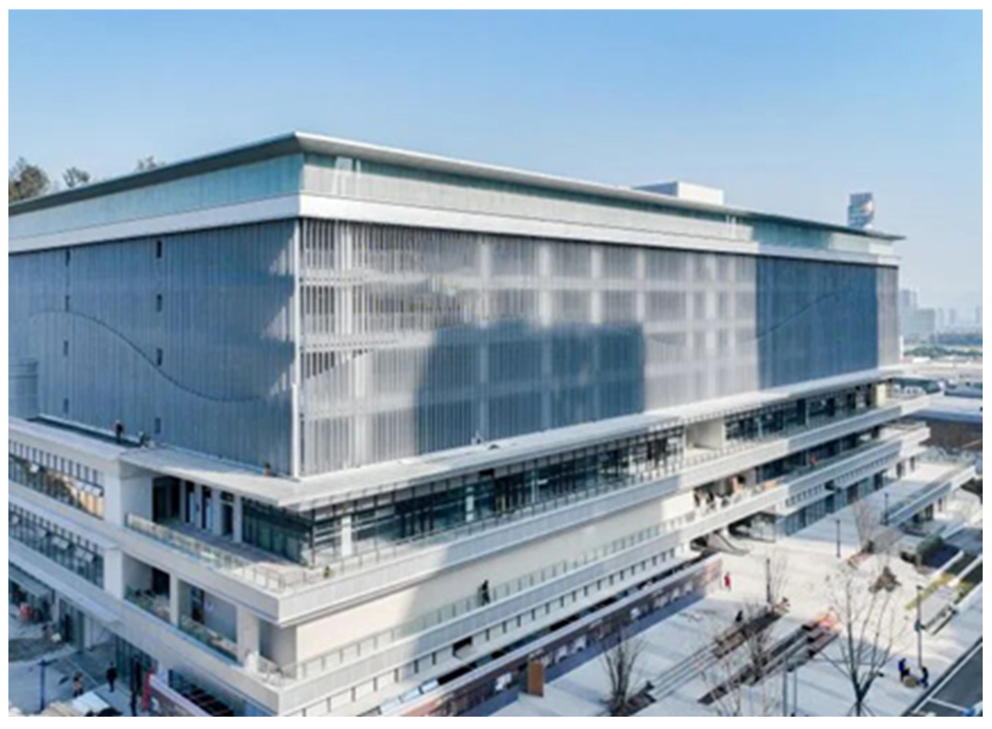
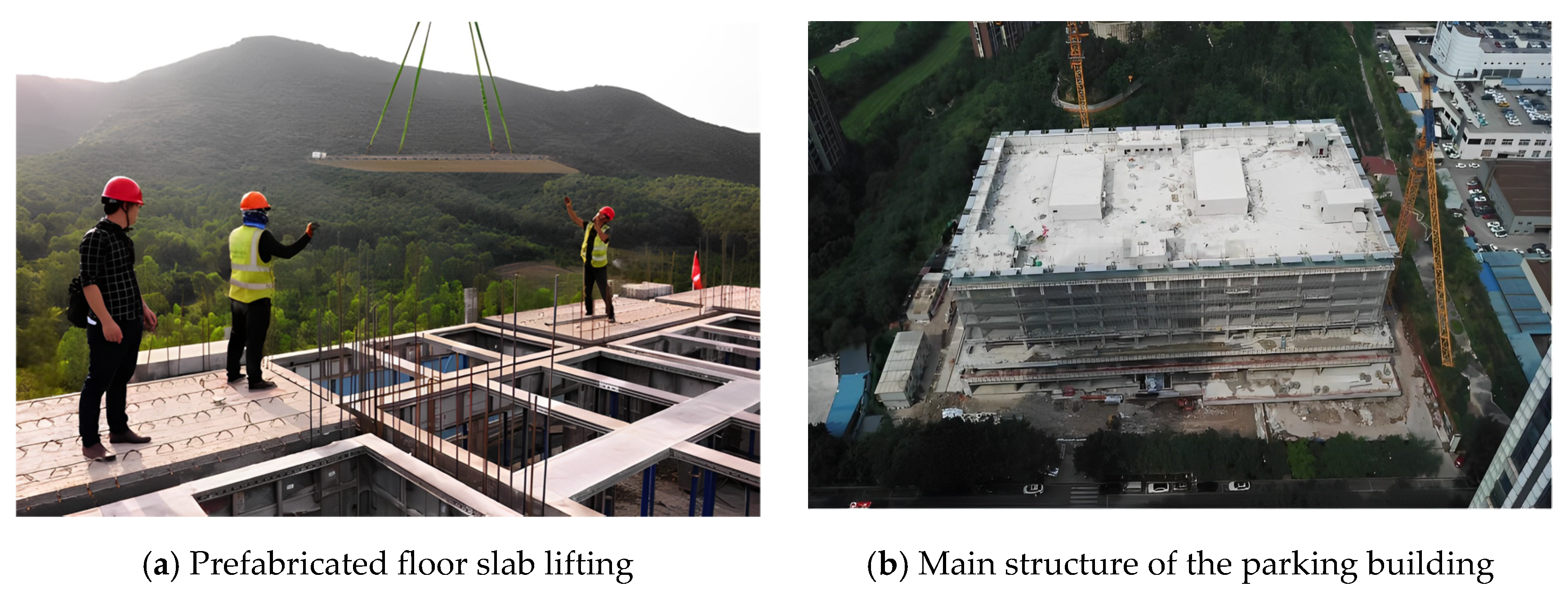
The improved quantification model was used to quantify the carbon emissions during the construction of a prefabricated public parking building, and a total of seven datasets were summarized, with floor as the variable. In order to expand the study samples, quantitative data on the carbon emissions during the construction of prefabricated buildings were collected from the existing research literature, and a total of 53 groups of data from quantitative studies were collected. The construction site of the prefabricated public parking building is shown in Figure 10.

After obtaining these 60 sets of quantitative data, the carbon emission impact parameter correlation was analyzed using the method in Section 3.2. The correlation heatmap is shown in Figure 11, and the results of the Pearson correlation test are shown in Figure 12.

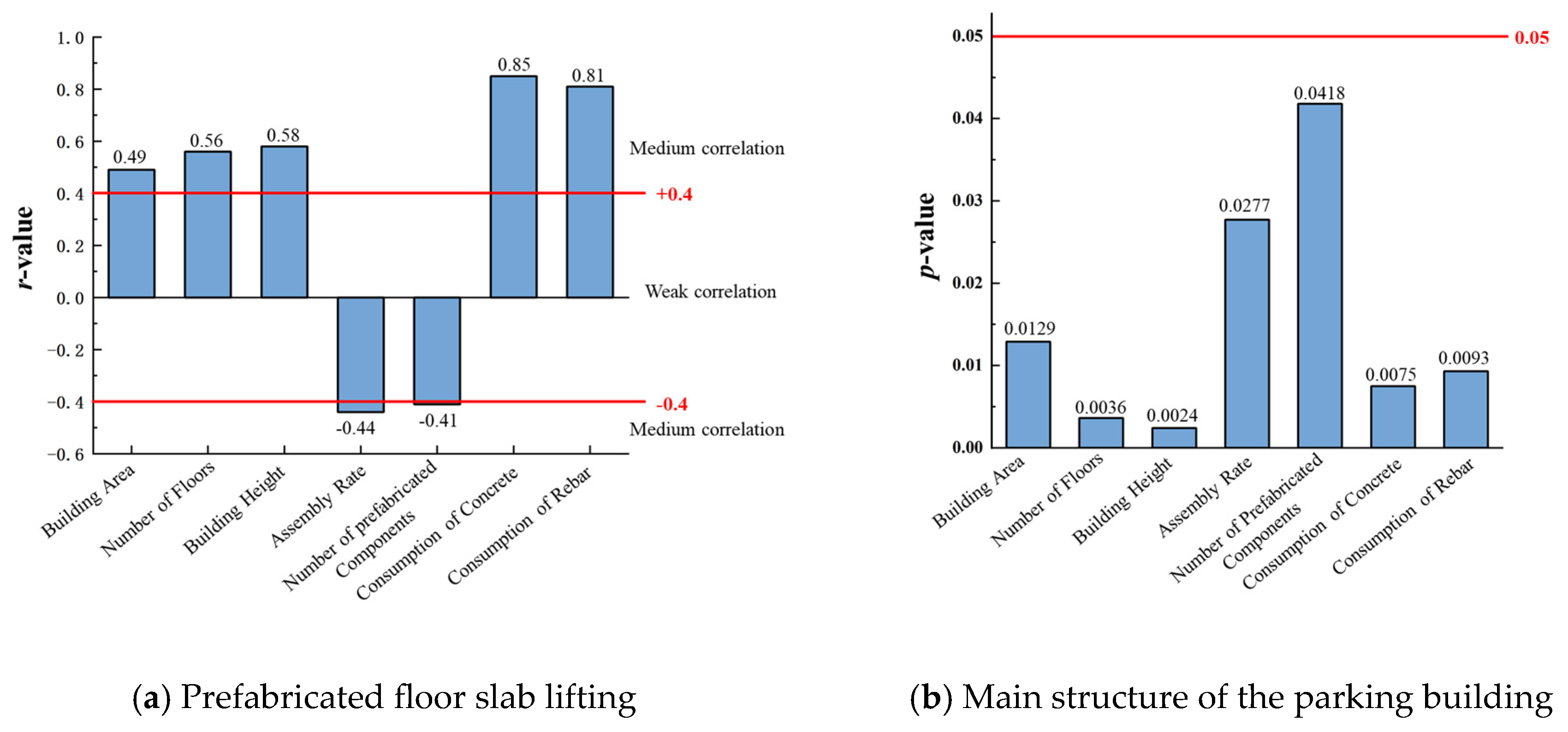
From the results of the Pearson correlation test in Figure 11 and Figure 12, it can be seen that the r-value is greater than 0.4 and the p-value is less than 0.05. According to the evaluation of r-value presented in the previous section, it can be seen that all seven variables have a significant correlation with the carbon emissions per unit area, and the correlation is above the medium degree. The r-value of the consumption of concrete and steel rebar is significantly higher than that of the other factors, in line with the dominant influencing factors of carbon emissions in building construction proposed by previous scholars [14]. Therefore, these seven influence parameters are the significant influence parameters governing the carbon emissions in the construction stage of the prefabricated parking building.

5.3.2. Data Expansion and Normalization

To ensure accurate differentiation between different predictive models, the training learning samples should be as large as possible. As there were only 60 groups of learning samples in this study, this may lead to a poor generalization ability in the prediction models. Therefore, the data interpolation method was used to expand the learning samples, and the original 60 groups of learning samples were expanded to 120 groups using the thin plate spline interpolation method.

Differences in magnitude between the impact parameters of carbon emissions will affect the accuracy of carbon emissions predictions, such as differences in the units of floor area and the assembly rate, as well as differences in the construction sites of the different prefabricated building projects. Therefore, the learning sample data were normalized before training to reduce the impact of the differences in the impact parameters, eliminate the effect of this magnitude, and improve the fitting effect of the model used to predict carbon emissions during the construction of prefabricated buildings. In this study, Min–Max normalization was used, the carbon emission learning samples were imported into the MATLAB R2022a program for normalization using the mapminmax function, and the mapping range of the feature parameters was set from 0 to 1. The partial results of the normalized data of the learning sample data are shown in

Table 2. Predictive model normalized data results.

No.	x1	x1	x1	x1	x1	x1	x1	y
1	0.4255	0.8927	0.9157	0.3418	0.7904	0.0687	0.7486	0.9389
2	0.2602	0.4350	0.5946	0.1807	0.9960	0.7615	0.8165	0.6697
3	0.2430	0.1821	0.9486	0.3167	0.5773	0.4127	0.4838	0.0412
4	0.1795	0.0269	0.1137	0.6050	0.7823	0.7847	0.5547	0.1254
5	0.1494	0.9091	0.4665	0.6505	0.9764	0.2255	0.8639	0.7207
·······                                                          ·····
116	0.2863	0.7887	0.2723	0.2721	0.8069	0.2148	0.2221	0.7803
117	0.1025	0.8048	0.5241	0.5639	0.7402	0.2837	0.8635	0.2216
118	0.3275	0.9580	0.9135	0.5971	0.6196	0.7349	0.8863	0.7740
119	0.3979	0.9641	0.5822	0.1671	0.8566	0.8972	0.7252	0.0091
120	0.1567	0.6210	0.0803	0.5532	0.0405	0.7562	0.3547	0.5244

.

5.3.3. Hyperparameter Optimization Results

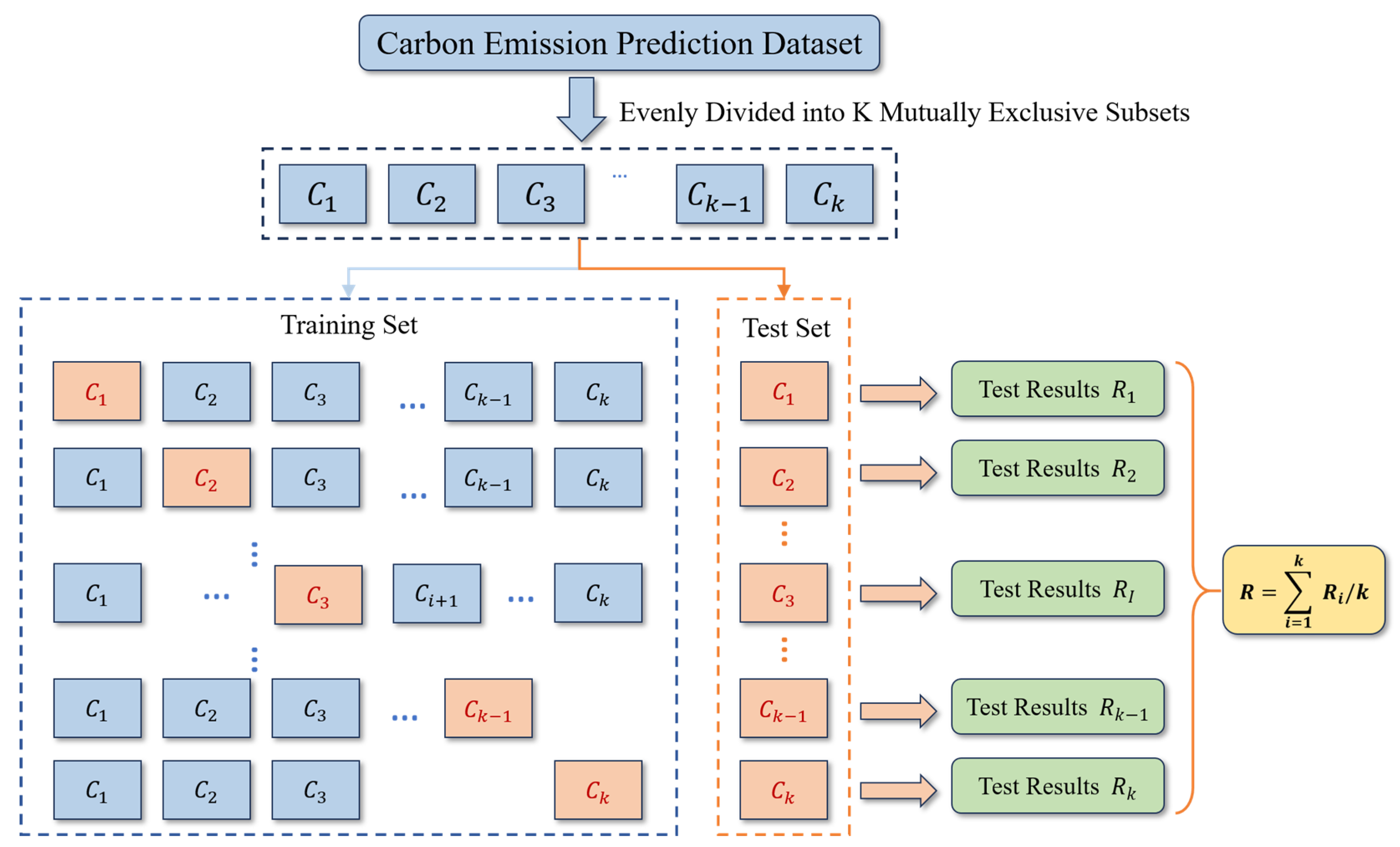
To predict the carbon emissions during the construction stage of prefabricated buildings, the optimal hyperparameters of four models, namely, SVR, BPNN, ELM, and RF, were determined using the lattice optimization and k-fold cross-validation methods. The number of cross-validation folds (k) was set to 3, 4, 5, and 6, respectively, and the Root Mean Square Error (RMSE) was used as the evaluation index. Theoretically, the closer the RMSE value is to 0, the smaller the model prediction error, and the more ideal the selected hyperparameter setting.

• (1) SVR prediction model parameter optimization

The key hyperparameters of the SVR include penalty factor C and the kernel function scale parameter γ. In order to determine the optimal combination of hyperparameters, the optimization range of the penalty factor C was set to 0.1~10 with a step size of 0.1, and the optimization range of the kernel function scale parameter γ was set to 0.01~1 with a step size of 0.01. The optimal parameter settings with different cross-validation folds were statistically analyzed using the grid optimization method. The results of the grid optimization and the optimal parameter settings are shown in Figure 13 and

Table 3. Results of the parameter optimization for the SVR carbon emission prediction model.

Cross-Validation Folds k	Optimization Time/s	Penalty Factor	Kernel Function Scale Parameter	RMSE
3	17.25	0.7	0.05	0.454
4	17.54	0.7	0.10	0.407
5	19.15	0.4	0.15	0.435
6	20.87	1.3	0.03	0.435

.

As can be seen from Figure 13, in all four cases of cross-validation, the value of RMSE shows a tendency to first decrease and then increase with the increase in penalty factor C and kernel function scale parameter γ. As can be seen from Table 3, the RMSE shows a tendency of decreasing and then increasing with the increase in the number of cross-validation folds. The optimal parameter search resulted in a value of 0.7 for the penalty factor C and of 0.1 for the kernel function scale parameter γ. At this time, the RMSE was the smallest, at 0.407, and the number of cross-validation folds, k, was 4.

• (2) BPNN prediction model parameter optimization

For BPNNs, the number of hidden layers, the number of hidden layer nodes, and the learning rate are key parameters that determine their complexity and performance. The selection of these parameters directly affects the prediction ability and convergence speed of BPNNs. Due to the limited number of learning samples, the hidden layer configurations of BPNNs are only considered for single-layer and double-layer cases. The number of nodes in a single hidden layer and the number of nodes in two hidden layers, as well as the learning rate of the BPNN, are optimized using grid optimization and the k-fold cross validation method. The optimization range of the number of hidden layer nodes was set to 1~50 with a step size of 1. The optimization range of the learning rate was set to 0.0002~0.01 with a step size of 0.0002. The number of network training times was set to 1000. The optimal parameter settings under different cross-validation methods were categorized and counted; the optimization results are shown in Figure 14 and Figure 15, and the optimal parameters for optimization are shown in

Table 4. Results of parameter optimization for the BPNN carbon emissions prediction model (single hidden layer).

Cross-Validation Folds k	Optimization Time/s	Number of the Hidden Layer Nodes	Learning Rate	RMSE
3	1353.69	12	0.0094	0.452
4	1161.17	14	0.0048	0.415
5	1272.17	3	0.0020	0.425
6	1298.07	10	0.0096	0.423

and

Table 5. Results of parameter optimization for the BPNN carbon emission prediction model (two hidden layers).

Cross-Validation Folds k	Optimization Time/s	Number of Nodes in the First Layer	Number of Nodes in the Second Layer	Learning Rate	RMSE
3	90682.01	50	4	0.0004	0.399
4	112589.43	5	32	0.0098	0.327
5	134175.03	13	13	0.0030	0.348
6	158175.03	12	7	0.0022	0.351

.

As can be seen from Figure 14, there is no obvious linear relationship between the prediction accuracy of the BPNN, the number of hidden layer nodes, and the learning rate. In the optimization search range, the RMSE is small when the learning rate and the number of hidden layer nodes are small, and large when the learning rate and the number of hidden layer nodes are large. As can be seen from Table 4, with the increase in the number of cross-validation folds, the RMSE shows a trend of decreasing and then increasing. The optimal parameter search results for the single hidden layer were as follows: the number of hidden layer nodes is three and the learning rate is 0.0020. The RMSE was minimized to 0.415 and the number of cross-validation folds, k, was 4.

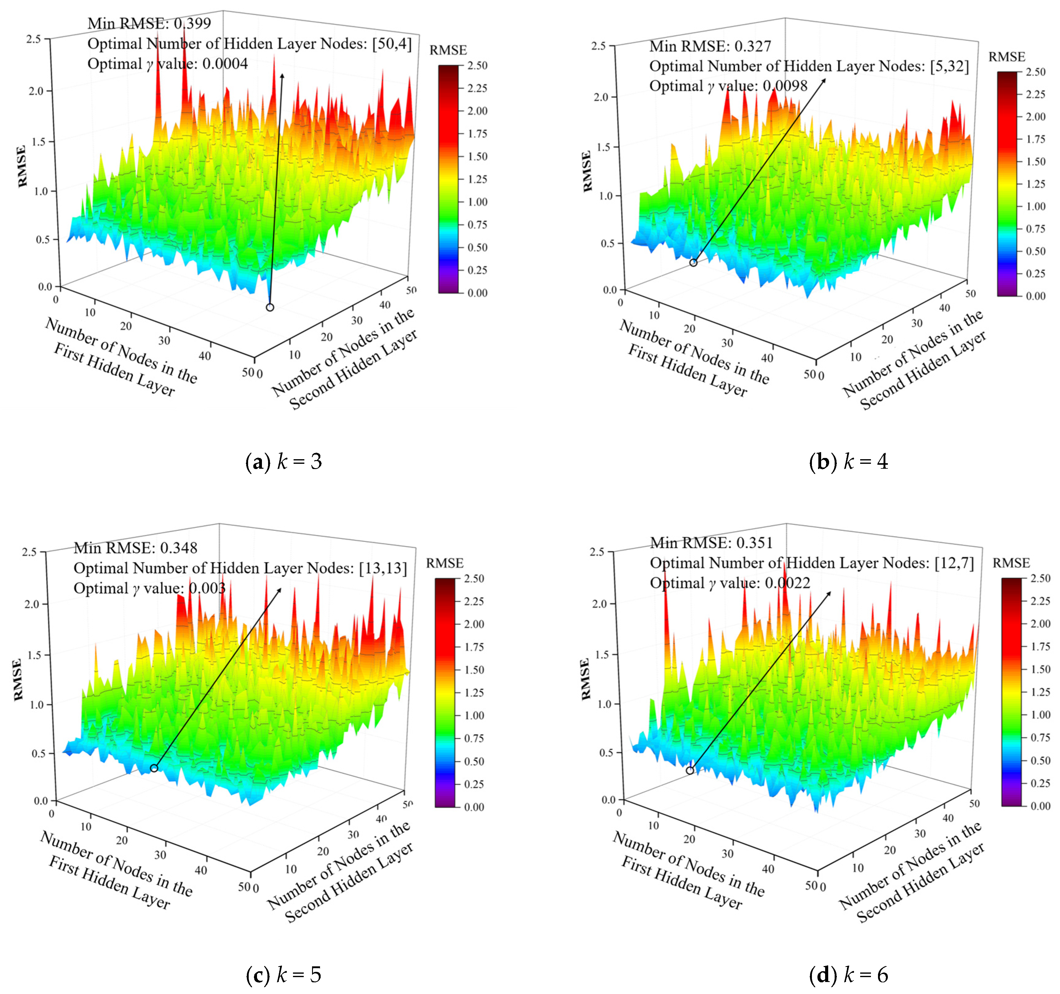
Comparing Figure 14 and Figure 15, it can be seen that there is a great deal of randomness in the influence of the number of nodes in the hidden layer and the learning rate of the BPNN on its prediction accuracy, but with the increase in the number of cross-validation folds, the range of the distribution of the RMSE gradually decreases and then increases in the range of the number of nodes searched. The overall prediction effect of the BPNN with two hidden layers is better than that of the one with a single hidden layer. The final selected BPNN parameters were as follows: two hidden layers, 5 and 32 nodes in the hidden layers, and a learning rate of 0.0098, with four cross-validation folds and an RMSE of 0.327.

• (3) ELM prediction model parameter optimization

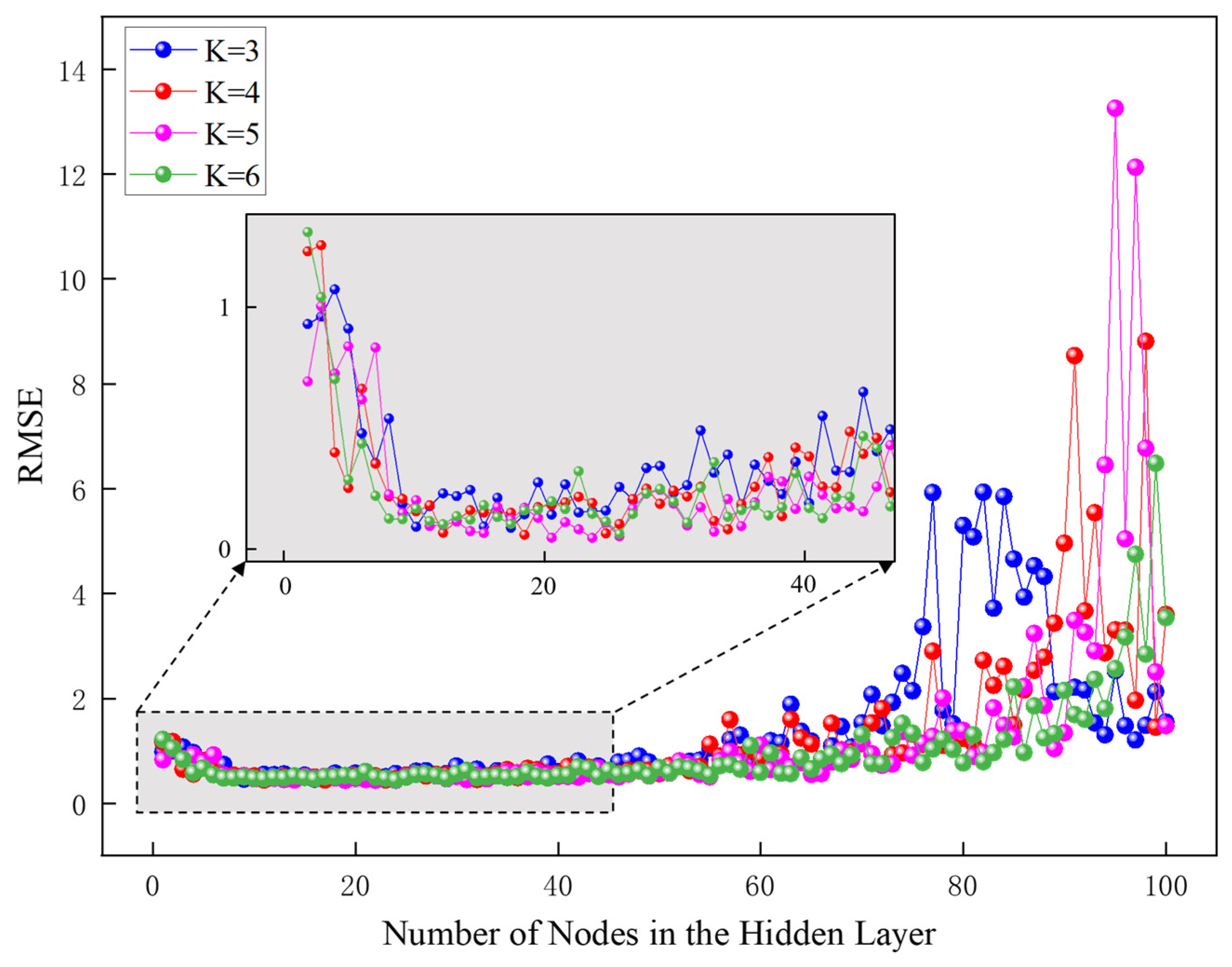
The main parameter to be adjusted for the ELM model is the number of implied nodes. In order to find the optimal parameter settings, the number of implied layer nodes n was set to 1~100, and the step size was 1. The optimal parameter settings under different cross-validation techniques were categorized and counted. The results of the search for optimality are shown in Figure 16, and the results of the search for the optimal parameters are shown in

Table 6. Results of parameter optimization for the ELM carbon emissions prediction model.

Cross-Validation Folds k	Optimization Time/s	Number of Hidden-Layer Nodes	RMSE
3	16.3	16	0.456
4	14.1	17	0.439
5	13.7	22	0.430
6	11.4	24	0.441

.

As can be seen in Figure 16, under the four cross-validation conditions, as the number of nodes in the hidden layer increases, the RMSE value shows a tendency to stabilize and then increase with oscillations. As can be seen from Table 6, there is no obvious trend in RMSE as the number of cross-validation folds increases. The optimal parameter search obtained 22 nodes in the hidden layer, at which time the RMSE was 0.430 and the cross-validation discount was 5.

• (4) RF prediction model parameter optimization

In the RF prediction model, the number of decision trees (n) and the minimum number of leaves (leaf) are two important parameters; a larger n can improve the accuracy of the model but can also increase the computation time, and a larger leaf prevents overfitting but may also lead to the underfitting of the model, so it is necessary to optimize parameters n and leaf of the RF carbon emissions prediction model. Since the number of learning samples was 120, the range of n was set to 1~30 and the step size was set to 1, while the range of leaf was set to 1~30 and the step size was set to 1 for optimization [34]. The results are shown in Figure 17, and the optimal parameter settings under cross-validation folds are shown in

Table 7. Results of parameter optimization for the RF carbon emissions prediction model.

Cross-Validation Folds k	Optimization Time/s	Number of Decision Trees	Minimum Leaf Number	RMSE
3	356.1	16	3	0.480
4	371.7	6	5	0.463
5	398.0	12	10	0.498
6	402.0	20	1	0.502

.

As can be seen from Figure 17, the RMSE decreases with an increase in leaf and increases with n. In Table 7, it can be seen that the model’s prediction is best when leaf is set to 6 and n is set to 5, and the model’s minimum error RMSE is 0.463 when the number of cross-validation folds is four.

5.3.4. Analysis of Carbon Emission Prediction Results

According to the optimization search results in Section 5.3.3, the four machine learning algorithms, namely, SVR, BPNN, ELM, and RF, have the smallest prediction model error for carbon emissions during the construction of prefabricated buildings when the cross-validation fold k is 4. In order to compare the effects of the four models’ predictions of carbon emissions during the construction of prefabricated buildings under the same conditions, the learning samples were divided into a training set and test set and numbered from 3 to 1. The model training samples were divided into 120 groups, with 90 groups functioning as training sets and 30 groups as test sets. The parameters of the model were set according to the minimum RMSE when the cross-validation discount k was 4. The evaluation indexes of the carbon emissions prediction model are the RMSE and the goodness-of-fit coefficient (R²); the smaller the RMSE, the smaller the model error, and the closer the R² is to 1, the higher the prediction accuracy of the model [35,36]. The carbon emissions in the figure are normalized carbon emissions. The carbon emission prediction results are shown in Figure 18, a comparison between the predicted and actual values of carbon emissions is shown in Figure 19, and a comparison of the carbon emissions prediction model performance indicators is shown in

Table 8. Comparison of carbon emissions prediction model performance indicators.

Prediction Model	RMSE	R2
SVR	0.385	0.859
BPNN	0.364	0.878
ELM	0.404	0.848
RF	0.413	0.841

.

In Figure 18, the RMSE of the SVR prediction model is 0.385, the RMSE of the BPNN prediction model is 0.364, the RMSE of the ELM prediction model is 0.404, and the RMSE of the RF prediction model is 0.413. Judging from the RMSE, the BPNN prediction model obtains the best results in the prediction of carbon emissions, with the smallest error. The RF prediction model obtained the worst carbon emission prediction results, which coincides with the optimal hyperparameter optimization search results in Section 5.3.3.

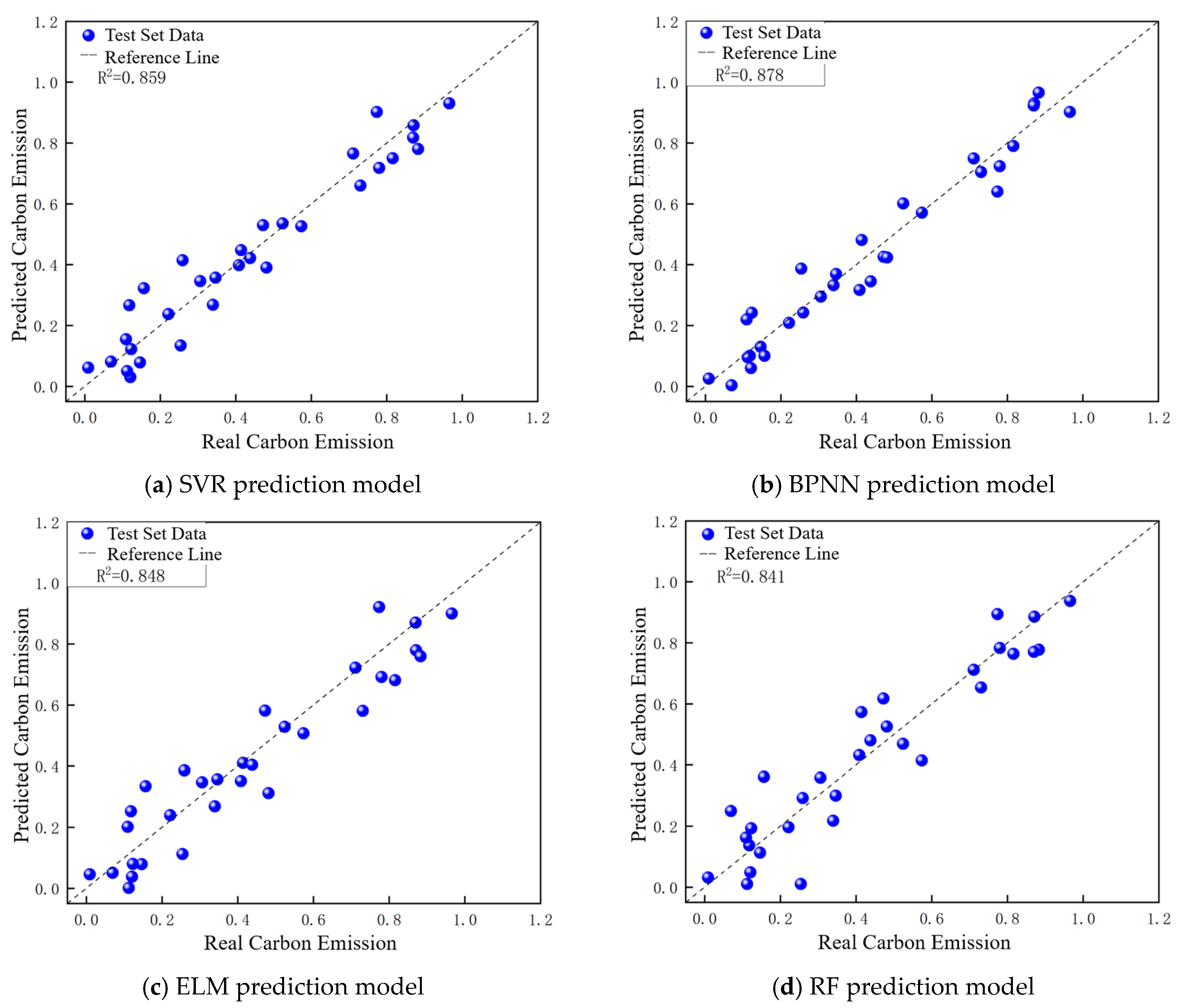
In Figure 19 and Table 8, it can be seen that the R² of the SVR prediction model, the BPNN prediction model, the ELM prediction model, and the RF prediction model are 0.859, 0.878, 0.848, and 0.841, respectively. The points of comparison between the predicted carbon emissions value and the actual value obtained by the BPNN prediction model are more concentrated on the reference line, the coefficient of goodness-of-fit is lower, and the prediction of the carbon emissions effect is the best. These results further validate the significant advantage of BPNN in capturing higher-order nonlinear relationships. Its core mechanism enables it to dynamically and iteratively optimize the weights via a back-propagation algorithm to more accurately model the complex correlation between the input parameters and carbon emissions [37,38]. In Figure 19b, it can be seen that the comparison points between the predicted and actual values of carbon emissions obtained by the BPNN prediction model are uniformly distributed on both sides of the reference line, which indicates that the amount of carbon emissions has no effect on the results of the prediction model, that the model’s predictions of carbon emissions show good stability, and that it has good applicability.

6. Conclusions

This paper provides a reliable method for quantifying and predicting carbon emissions during the construction of prefabricated buildings, thus providing a strong guide for carbon reduction strategies in building design and construction management. The main conclusions of this paper are as follows.

The system boundary of the carbon emissions during the construction of prefabricated buildings study was established from the time dimension and the space dimension. The temporal boundary of carbon emissions quantifications was the construction of prefabricated buildings, including the foundation construction stage, the construction of the main part of the building, the decoration construction stage, the electromechanics installation construction stage, and the disposal of construction waste. The space boundary mainly focused on the construction site where the construction activities took place, and the transportation routes of building materials and prefabricated components from the factory to the construction site were also included in the research scope of quantifying carbon emissions during the construction stage.

The traditional carbon emissions quantification model could be improved via the process analysis method and the carbon emissions factor method. The construction of the main structure of prefabricated buildings was taken as the core, and the quantification model was divided into seven modules: the earthwork and foundation pit engineering module, the foundations and piling engineering module, the cast-in-place reinforced-concrete engineering module, the prefabricated engineering module, the decoration engineering module, the electromechanics installation engineering module, and the construction waste disposal module. Each module underwent a separate analysis.

Based on the proposed basic-element concept and its coding rules, a quantitative calculation of the matrix product was applied to itemize the carbon emissions during the construction of prefabricated buildings, which simplified the process of quantifying carbon emissions and solves the shortcomings of the traditional full-life cycle quantification method, which suffers from large deviations.

Following a correlation analysis of the influence parameters, the results of the Pearson correlation test revealed an r value of greater than 0.4 and a p value of less than 0.05. Seven variables showed a significant correlation with carbon emissions per unit area, and the correlation was above the medium degree; therefore, it was determined that the building area, the number of floors, the building height, the assembly rate, the number of prefabricated components, the consumption of concrete, and the consumption of rebar seven variables can be used as impact parameters to measure carbon emissions during the construction of prefabricated buildings.

The carbon emissions prediction model focusing on prefabricated buildings’ construction stage, based on four machine learning algorithms, was established. Based on the identified carbon emission impact parameters, a database of quantitative samples was created by applying the improved quantitative method, and the 60 sets of data were expanded to 120 sets using the thin plate spline interpolation algorithm.

Grid optimization and k-fold cross-validation were used to find the optimal hyperparameters of the model, compare the RMSE index of each result, and choose the optimal number of cross-folds, which was selected as four. By calculating and analyzing the RMSE and R² of the prediction results of the four models, it was concluded that the RMSE value of the BPNN is the smallest, at 0.364, indicating that its prediction has the fewest errors and the R² of the BPNN was closest to 1, 0.878, indicating that its prediction obtained the highest accuracy. The results show that the BPNN model that was constructed based on the modular quantization method is consistent with previous research results [39], demonstrates high prediction accuracy, and has good applicability in the prediction of carbon emissions during the construction of prefabricated buildings.

The method proposed in this paper to quantify the carbon emissions produced during the construction of prefabricated buildings can be used to accurately calculate the carbon emissions of different modules during the construction stage of actual projects. This method not only significantly improves the efficiency and accuracy of these calculations, but also can analyze the individual modules in detail, making it more flexible and practical than the traditional overall calculation method. In addition, using the carbon emissions prediction model proposed in this paper to determine emissions during the construction of prefabricated buildings could greatly improve the efficiency of prediction and provide scientific and powerful guidance for the formulation of carbon emission reduction strategies in building design, construction management, etc., which is of great significance for promoting green and low-carbon engineering construction.

Although the carbon emissions prediction model focusing on prefabricated buildings’ construction stage presented in this study achieved excellent results and showed practical value, there is still potential for further research on the number of datasets used and the dominant factors contributing to carbon emissions, and later studies could consider more advanced algorithms to optimize the model.