Article

Grey-Box Model for Efficient Building Simulations: A Case Study of an Integrated Water-Based Heating and Cooling System

1
Institute of Thermal Engineering, Graz University of Technology, Inffeldgasse 25b, 8010 Graz, Austria
2
BEST—Bioenergy and Sustainable Technologies GmbH, Inffeldgasse 21/B, 8010 Graz, Austria
*
Author to whom correspondence should be addressed.
Buildings 2025, 15(11), 1959; https://doi.org/10.3390/buildings15111959
Submission received: 25 March 2025 / Revised: 23 May 2025 / Accepted: 31 May 2025 / Published: 5 June 2025
(This article belongs to the Section Building Energy, Physics, Environment, and Systems)

Abstract

:
Efficient and accurate grey-box building models, including water-based heating and cooling systems, are crucial for simulating and optimizing the energy demand of building, neighborhood, and network scenarios. However, the numerical effort and the amount of input data required for existing models are still high, and the parameterization of these systems is very labor-intensive. This paper presents a grey-box model that addresses these limitations by requiring minimal input data and offering a highly efficient parameterization method. Using physical principles, the model was validated against a detailed physical building model and measurement data. Our results show that the grey-box model accurately predicts return temperatures (σ = 0.37 K, µ = 0.05 K) and room air temperatures (σ = 0.62 K, µ = 0.28 K). Compared to 8229 s for the detailed physical model, the model requires only 18 s for a one-year simulation. The model also shows robust behavior with alternative weather data and control strategies. The key contribution of this work is the development of a grey-box model that combines high accuracy and numerical efficiency with significantly reduced data and parameterization requirements, with possible applications in large-scale building simulations, demand-side management, short-term energy storage strategies, and model predictive control.

1. Introduction

1.1. Context

The building sector significantly impacts global warming due to its high energy consumption, which leads to greenhouse gas (GHG) emissions. This sector accounts for approximately 40% of the total energy consumption and is responsible for about one-third of GHG emissions [1]. These GHG emissions contribute to climate change and global warming. Additionally, climate change increases the frequency, duration, and intensity of weather extremes, such as heat waves [2]. Therefore, reducing energy consumption and, consequently, GHG emissions is imperative.
Transitioning to a low-carbon heating sector requires the use of a combination of increased energy efficiency measures, a higher share of renewable heat, and sector coupling. Potential energy savings can be achieved through intelligent control strategies for heating and cooling systems, which utilize the building storage mass for short-term energy storage [3]. Other possibilities include peak demand reduction [4] and energy consumption forecasting [5].
To better understand and be able to define the reduction potential of GHG emissions in the building sector, building energy modeling (BEM) is often employed. In essence, BEM provides a virtual environment to test and analyze different scenarios related to building energy performance. BEM can be used for energy demand modeling, life cycle assessment, and economic analysis. Energy modeling is also used at the neighborhood [6,7] and urban levels [8,9,10] (urban building energy simulation models, UBEM), considering dynamic interactions between heat generation, the district heating network, and the buildings and their heat emission systems.
The results depend heavily on the quality of the used building model [11]. In the field of building energy modeling, simulation models are classified into two main types, namely white-box and black-box, and an intermediate type, grey-box (GB) models. The selection of a particular modeling approach depends on project-specific requirements, data availability, and the balance between accuracy, computational efficiency, and interpretability.

1.2. Literature Review

There are two main categories of building simulation models: white box and black box models. The choice of which of these to use depends significantly on the project requirements and available data. White-box models, also known as “Forward” models [12], are based on physical principles, incorporating the laws of heat transfer and thermodynamics. These models are often used in building simulation programs, such as EnergyPlus, TRNSYS, and Modelica [13]. While this type of model typically provides reliable simulation results, it requires a wealth of information about the building to determine all necessary parameters, which can be time-consuming and not cost-effective. Another drawback is the relatively long calculation time required, which makes control optimizations and network simulations numerically intensive or impossible. Data is used for calibration to adjust specific, uncertain physical parameters, such as heat transfer or infiltration rates [14].
Black-box models are “Data-driven”, relying solely on input–output data to generate predictive outputs without needing explicit knowledge of underlying physical processes. They are pure data-in–data-out models and include neural networks [15] and/or support vector machines [16], which are numerically highly efficient. However, many other examples exist, including but not limited to: random forests, gradient boosting machines, and naïve Bayes.
GB models represent an intermediate stage, combining the strengths of both white-box and black-box approaches. They offer greater numerical efficiency and simplicity than white-box models, and compared to black-box models, the results can be more easily interpreted thanks to their grounding in physical principles. GB models can also more effectively predict behavior when different control strategies are applied [17]. Numerous studies have focused on determining the ideal number of C (capacity) and R (resistance) elements in GB models [18,19,20,21,22]. A common recommendation made by many researchers is to use two capacitances, as they find that increasing the number of capacitances beyond this number does not significantly improve the modeling results. These simplified physical structures have aggregated parameters, such as total thermal resistances R and heat capacities, that can be estimated from measured data [23,24].
Reynders et al. [25] developed reduced-order GB models using data-driven system identification to address unknown thermal properties. The models were evaluated for prediction accuracy and parameter interpretation based on simulation data. The impact of dataset choice and data quality, including noise, on model performance was assessed.
Linear GB models are widely found in the literature [26,27]. These models assume linear relationships between the input and the output. Yanfei et al. [28] studied existing GB models and their usage, revealing that only a few studies used “Forward Approach” models, which derive parameters for R and C based on physical laws. Most studies rely on an “Inverse Method”, which is data-driven [29,30].
Thilker et al. [31] developed a nonlinear GB model based on stochastic differential equations using an “Inverse Approach”. They also integrated a water-based radiator system, which could accurately predict room temperatures, return temperatures, and heat outputs in an unoccupied school building over a week. He also found that solar radiation does not significantly influence the model. One limitation of their approach is the need for extensive data to identify the model’s parameters.
Harb et al. [32] studied a model identification approach for forecasting the thermal behavior of a building. He discovered that an R4C2 approach yields the most accurate indoor climate forecasting results. The model uses linear convective heat exchange between the air and the wall and uniformly distributed properties for all building components.
Berthou et al. [33] analyzed four GB models without water-based heat emission systems. They found that an R6C2 model is sufficient when thermal demands are high. The authors recommend using a separate model parameter set for every month, which requires a separate identification process for each individual month.

1.3. Research Gaps and Research Objective

White-box building simulation models, while theoretically capable of representing building physics, often require a large amount of detailed information about the building’s structure and systems. This data intensity makes them time-consuming and costly to implement, especially at the neighborhood or city scale.
For black-box models, data are often not available in sufficient quality and scope, especially on a neighborhood level, including old buildings with limited or no documentation. The use of insufficient data can lead to inaccurate results and an inability to generalize the results to different operating conditions. Detailed performance data for heating systems or room temperatures are rarely available at the neighborhood and urban levels. However, even with adequate amounts of data, the parameterization of black-box models remains a significant challenge. This is particularly due to the fact that real buildings are often controlled to maintain a stationary operating point, rather than to capture and respond to dynamic behavior. This makes the calibration of black-box models more difficult, as they must adequately represent the complex and variable nature of building dynamics, which is far beyond maintaining a constant state.
This problem also affects GB models, but they offer a potential solution through the combination of physical principles with data-driven approaches. However, significant research gaps remain, particularly in the application of physical principles to GB models for heating and cooling systems. There is a notable lack of models capable of handling water-based systems under design conditions, especially in the context of district heating.
In addition, most studies compare GB models to a reference model or measurement over short time periods, typically covering only a single heating or cooling season. A comprehensive evaluation, however, is crucial to ensure that building models produce reliable simulation results. Limited time frames often capture only a narrow range of boundary conditions, increasing the risk of overfitting. When extensive data for black-box models is unavailable, GB models—with their lower parameter requirements and integration of physical principles—serve as a practical alternative for feasibility studies. These studies become more informative and yield more reliable results when models are tested under diverse conditions, such as varying weather patterns or supply temperature fluctuations. In contrast to many existing GB models, our approach has more physically interpretable variables tailored to water-based heating systems. The model is calibrated and validated against both a detailed white-box model and experimental data from an office building. This provides a more direct physical interpretation and potentially improves the handling and calibration workflow.
This paper presents the following main contributions:
  • Creation and validation of a detailed building model of a campus building at the Campus Inffeldgasse of Graz University of Technology using data from IoT sensors for calibration and validation;
  • Development and comprehensive comparison of a GB model based on physical laws, incorporating a water-based heat distribution system for both cooling and heating purposes;
  • A comprehensive comparison of the GB model with the detailed building model and measurement data, focusing on heat flows, room temperatures, and return temperatures of the radiator system;
  • Evaluation of the model’s robustness through simulations with alternative control methods and weather files;
  • A sensitivity analysis using the Morris Method to identify key model parameters for calibration and discussion of the model’s applicability to various building types and district heating systems.
First, Section 2 provides a detailed description of the developed white-box and GB building models, including the parameter identification process and the evaluation of the robustness of the GB model. Section 3 presents a case study where the developed models are compared with each other and validated using real-world measurement data. Finally, Section 4 summarizes the main findings, draws conclusions, discusses limitations, and provides an outlook on future research directions.

2. Modeling Approach

To provide an overview of the workflow used, the used methodology is shown in Figure 1, Figure 2 and Figure 3. The first step was to create a detailed building model, which was accomplished using the software IDA ICE [34]. The detailed model was created to enable a detailed comparison to the grey box model, as unfortunately, there was a lack of detailed experimental data from the building over a longer period of time. Parameter identification and validation for the detailed model were conducted in two stages. The first stage was carried out by performing an experiment in which a building was continuously heated up with a high supply temperature for 24 h and then allowed to cool down for 36 h over a weekend. In a second stage, the detailed building model was calibrated with data for monthly heating and cooling energy measurements in the year 2021.
The developed GB model was established in two versions: GB1, for which the parameters were identified using the results from the detailed model, and GB2, using experimental data. The second step (Figure 2) was achieved by comparing the results from the GB1 model with those from the detailed model and formulating an optimization problem. Furthermore, the parameters for the GB2 model were also identified using measured data, which included heat flows collected over a two-month period that included cooling, heating, and transition periods (third step). In formulating the optimization problem, an attempt was made to use the information available for the respective comparison model for each model. This resulted in different target functions to avoid overfitting and to speed up the identification process.
In the fourth step (Figure 3), the robustness of the GB model was analyzed. Two additional variants were defined for the comparison of the GB1 model with the detailed model. For this purpose, the validated models (both detailed and GB1) were simulated and compared using different weather data and an alternative control strategy. Finally, the calibrated GB2 model was compared with real-time measured data to assess its suitability for other applications.
Furthermore, a sensitivity analysis was performed using the Morris method [35]. This method helps to quickly identify the most influential parameters of a function by allowing the user to evaluate the mean of the absolute values of the elementary effects (µi*), while the standard deviation (σi) measures interactions and non-linear effects. This analysis is critical for subsequent investigations, and the insights gained allow the researcher to gain a better understanding of the GB model. Knowing the effects of key parameters and accurately setting bandwidths can significantly improve optimization problems. Furthermore, these findings can guide the direction of future research efforts. To apply the Morris method, the SaLib Python library v1.4.6 was used [36].

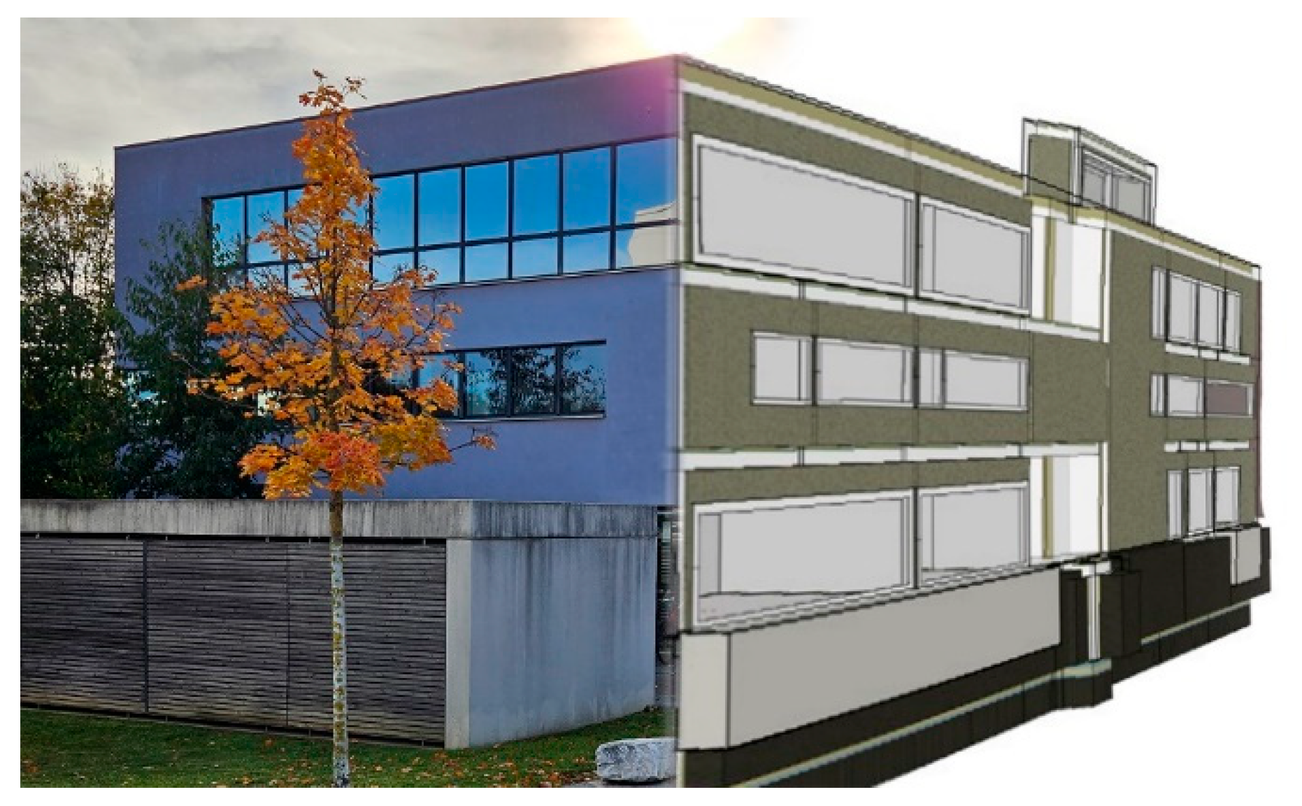
2.1. Reference Building

The considered building is an office building situated on one of the campuses of the Graz University of Technology (Figure 4). The structure consists of four floors with a total height of 12 m above ground level. It has a width of 15.7 m and a length of 43 m. The total floor area of the building is 2480 m2, which is divided as follows: 49% office space (38 rooms), 23% circulation areas, 9% storage, 3% common areas, 6% lecture halls and libraries, 0.5% technical facilities, 1.5% sanitary and other spaces, and 8% laboratories and workshops. The building has a heating demand of 59 kWh/(m2a) and a cooling demand of 51 kWh/(m2a). The cooling and heating capacities are limited to 70 kW each. Energy is supplied through a local heating and cooling network, with the heating and cooling facilitated via a pipeline, and two heat exchangers are used for the heating and cooling energy supply.
Concrete core activation provides heating and cooling for each floor. Each floor is supplied by a single motorized valve connected to the riser pipe. There is a total of four valves that can be centrally controlled. Currently, for the sake of simplicity, the valves are maintained in a constant position throughout the year, as the control of concrete core activation in the building has proven difficult in the past. Only the supply temperature is variably controlled based on the outdoor air temperature, for both heating and cooling purposes. Whether the system heats or cools is solely determined by the current outdoor air temperature. In the heating mode, the system activates the concrete core when the 24 h moving average outdoor air temperature falls below a threshold of 14 °C. In this mode, the temperature delivered to the concrete core depends on the current outdoor air temperature. This heating process remains active until the 24 h moving average outdoor air temperature exceeds 14.5 °C again. In the cooling mode, the system activates when the current outdoor air temperature exceeds 18 °C and deactivates when it falls below 16 °C. The current control system does not consider room air temperatures and does not allow for user intervention.

2.2. Metrics

To evaluate deviations and the model accuracy, the Root-Square Error (RSE), the Coefficient of Variation of the Root-Mean-Square Error (CV(RMSE)), and the Normalized-Mean-Bias Error (NMBE) were employed. ASHRAE Guideline 14-2014 [37] outlines the requirements for building simulation, which, for monthly calibration, stand at 15% CV(RMSE) and ±5% NMBE.
In this context, the variable y represents the comparative variable, and placing a circumflex (^) above it denotes the measured value. The notation ‘i’ represents the index variable iterating up to ‘n’, the total number of measurements. In the context of a monthly comparison, ‘n’ is the number of months, while in a time series analysis, it is the number of time steps. The mean of the measurements is denoted by µ.
R S E = i = 1 n ( y i y ^ i ) 2
C V ( R M S E ) = i = 1 n ( y i y ^ i ) 2 n μ · 100
N M B E = k = 1 n ( y k y ^ k ) n μ · 100

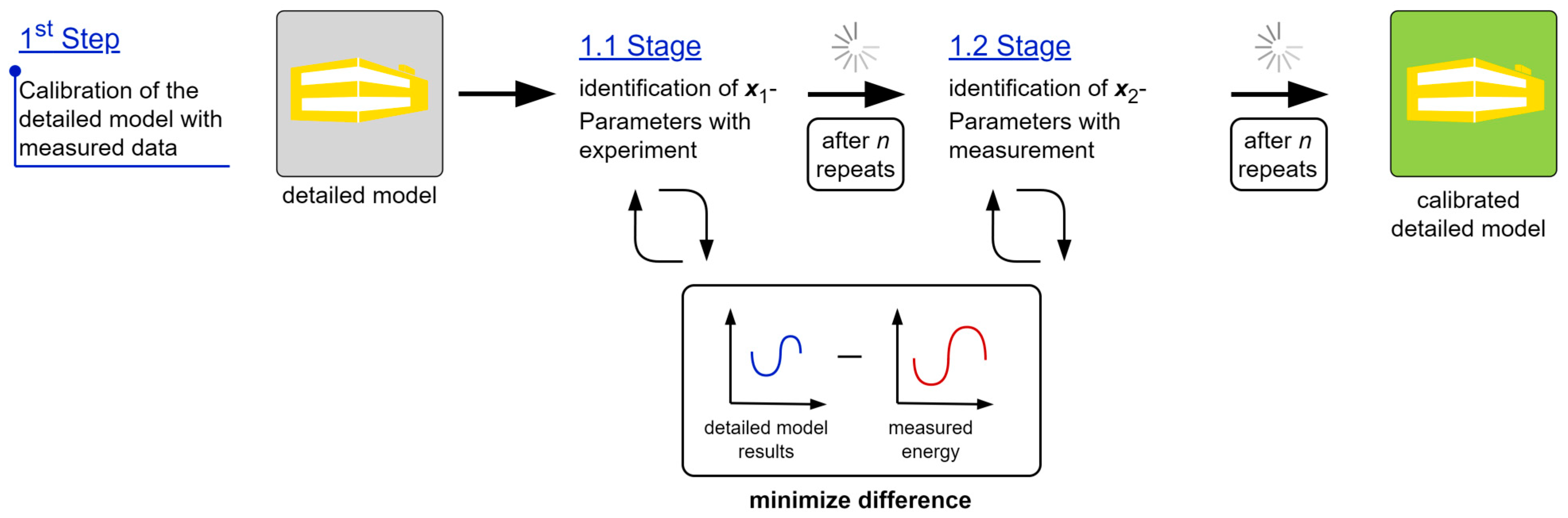
2.3. Step 1: Detailed Building Model

The detailed white-box building energy model (detailed model) was established using IDA ICE 5 Beta28 [34]. This approach was chosen to predict the thermal behavior without incorporating stochastic disturbances and uncertainties. To achieve this, measurement data provided by an IoT platform were used. These encompassed heating and cooling modes, valve positions per floor, surface temperature of the ceiling, supply and return temperatures, and the monthly energy consumption for heating and cooling. The volumetric flow rates were measured by detecting the mean pressure difference at a valve. Additionally, room temperatures were measured in two more spaces to ensure the accurate behavior of the model. Architectural and engineering documentation was used to extract the geometry and physical properties of the building.

2.3.1. Modelling Approach

The building was modeled on a room-by-room basis using IDA ICE. The corresponding usage categories were extracted from the university room book, and the vocabulary was based on DIN 277 [38]. Based on this vocabulary, usage categories were assigned according to SIA 2024:2021 [39]. Table A1 illustrates this assignment for the utilized usage categories. Each usage category incorporates internal loads and their schedules for occupancy, lighting, and devices.
The geometry was imported using a Building Information Modeling (BIM) model and the Industry Foundation Classes (IFC) interface into IDA ICE. The physical properties of the envelope were derived from the available energy certificate of the building, and the physical properties of the building’s component layers were sourced from ÖNORM B 8110-7:2013 [40]. Table 1 provides a summary of the physical building properties of the simulation model. For a detailed description of the modeling process, refer to [41].
The weather file was obtained from GeoSphere [42], the Federal Institute for Geology, Geophysics, Climatology, and Meteorology in Austria, through their API. The chosen location for the weather data is Graz University, which is situated 2.4 km away from the building site. All necessary data for modeling, except for direct normal radiation, were included in the file. The conversion to direct normal radiation was performed using the following equation:
E D N I = E G H I E D H I cos Φ
where the zenith angle is limited in the model to Φ < 88° to avoid unrealistically high values. Shading is activated when the outdoor temperature exceeds 25 °C or when the façade irradiance exceeds 200 W/m2. Window operation is controlled to maintain a balance between thermal comfort and air quality: They are opened when cooling is required and the air temperature difference between the inside and outside exceeds 2 K, or to ensure that CO2 levels do not exceed 1000 ppm. Cooling is required when the indoor temperature exceeds 26 °C.

2.3.2. Calibration of the Model Using Experimental Data

To perform the simulations, we anticipated that discrepancies between simulation and reality might arise due to simplifications in the modeling, the precision of parameterization, and the assumed boundary conditions. However, despite these potential discrepancies, the simulations were designed to provide a robust and reliable approximation of real-world scenarios. Thus, they provide valuable insights into system behavior and performance.
A good building model needs careful calibration to ensure that the room temperature, return temperature, and heat flow are as accurate as possible. The IoT platform was used to collect, extract, and process the sensor data required for verification. The sensor values included, among other parameters, the supply and return temperatures of the heat emission system, surface temperature of the ceiling for two rooms, and monthly energy consumption for heating and cooling.
The calibration of the IDA ICE model was performed using automatic multi-objective optimization (AutoMOO), an internal optimization algorithm in IDA ICE. Starting from one or more objective functions dependent on many parameters, the optimization process aimed to find solutions on the Pareto front, representing different trade-offs between the objective functions. AutoMOO encompasses various optimization methods. It is an evaluation algorithm that assesses optimization algorithms and selects the one that yields the best results for each run or generation. This capability not only ensures that many non-dominated solutions are found, but also that more complex models can be used with AutoMOO. For detailed information, refer to [34]. Model calibration was performed with two datasets. First, a calibration was conducted using experimental data, and second, a calibration was conducted using monthly cooling and heating energy data.
In the first stage (first step, Figure 1), measured data were used from a heating-up and cooling-down experiment that was conducted over a weekend. This time period, which might seem a bit short, was chosen in order to minimize the impact of the test on comfort, but it should be long enough to allow for significant temperature changes in terms of thermal inertia. Before the experiment, the volumetric flow rate for each floor was separately determined to define the design performance and establish bandwidths for the optimization problem. Subsequently, the bandwidths were narrowed by using Gaussian error propagation. In this study, measurement inaccuracies were considered, including instrumentation inaccuracies (1.00%) and valve flow tolerances according to manufacturer specifications (6.03%). The volumetric flow rates were measured by determining the mean pressure difference across an Oventrop Hydrocontrol VFC globe valve with an IMI TA-Scope measuring device. The error propagation of the individual floors was, for the ground floor, ±6.905%; the first floor, ±6.662%; the second floor, ±6.698%; and for the roof, ±7.063%. In the simulations, the measured time series of flow rate and flow temperature into the heat emission system were used as inputs.
The heating-up and cooling-down experiment started on 10 February 2023 at 17:30 and was carried out until 13 February 2023 at 05:30. For this purpose, the concrete core activation was supplied with an average flow temperature of approximately 32 °C for 24 h. The building was then cooled down for 36 h. To adjust the parameters, a multi-objective optimization approach with two objective functions was used. On the one hand, the difference between the simulated and measured return temperature in the heating-up phase was used, and on the other hand, the differences in the surface temperatures of the ceiling measured during the test were used (heating-up and cooling-down phases). Two more room temperatures were used for visual cross-validation. This means that the resulting temperature profiles for these rooms were compared with the measured data solely for visual assessment, but were not included in the parameter identification process itself. The optimization process was carried out to minimize the RSE over the considered period for the target functions (5)
min x 1 R S E T r e t , T ^ r e t ,   R S E T s u r f , T ^ s u r f   ,
where T ^ r e t and T ^ s u r f are the measured values for the return and surface temperatures, respectively. The vector x1 in Equation (5) corresponds to the parameters used in the simulation model that should be optimized. The vector includes the individual floor design power, the heat transfer coefficient of the concrete core activation, and the parameters influencing the thermal losses (thermal bridges, infiltration, and U-value). In addition, no specific algorithm has been used for determining the importance of each parameter. The limits for these parameters were taken from the default values within the simulation program, which are representative of the building type considered. In the first phase, 500 simulations were carried out with the multi-objective solver (AutoMOO). The selected parameter set chosen was the one that produced the minimum of the target function when both the RSE-functions were equally weighted, i.e., R S E T r e t , T ^ r e t + R S E T s u r f , T ^ s u r f .
In the second stage (first step, Figure 1), the vector of parameters, x1, obtained from the first stage, were used to calibrate the internal and external heat gains. This included all internal loads, which were adjusted in % relative to the specified standard values found in SIA 2024:2021 [39], and the solar heat gain coefficient (SHGC), as well as the transparency of the shading. This calibration was performed using the metrics CV(RMSE) and NMBE applied to the monthly heating and cooling energy data:
m i n x 2 C V ( R M S E ) h e a t , C V ( R M S E ) c o o l , N M B E h e a t , N M B E c o o l
where x2 is the vector that contains the parameters to be optimized. The calendar year 2021 was chosen as the simulation period. In the second phase, 280 simulations were carried out with the multi-objective solver (AutoMOO). The selected parameter set was the one that gave the minimum of the target function when the CV(RMSE) for heating and cooling were equally weighted, subject to the secondary constraint that the NMBE for heating and cooling met the ASHRAE requirements.

2.4. Grey-Box Model

This section describes the development process of the GB model. It begins with the presentation of the scheme in the form of an RC model, followed by the used differential equations. Each term in the equations is then explained in detail, and typical values are provided.

2.4.1. Model Formulation

The schematic representation of the RC model used for the GB model, using capacity nodes and resistances, is shown. RC models are a standard approach to representing the thermal behavior of buildings in GB models, as they provide a good balance between simplicity and accuracy. An emphasis has been placed on parameter descriptions that allow information to be extracted from various databases and geo-referenced information systems, thus facilitating its use in network simulations. Furthermore, to avoid overloading the model with parameters, only the essential parameters that adequately represent a building and its heat emission system should be extracted from these databases. This approach leads to a deeper understanding of the GB model and optimizes its use. Therefore, three resistances (3R) and a two-node system (2C) have been chosen for our model, as 2C has been shown in the literature [43,44] to give optimal results in terms of performance. The entire building is modeled with a single thermal zone.
In this context, Ta is the outdoor air temperature, Ta,eq is the equivalent outdoor air temperature, Ce is the capacity of the thermally active storage mass, Te is the temperature of the storage mass, Cin is the capacity of the air node, calculated by considering the air volume and its specific heat capacity, and additionally, the thermal capacity of the furniture. Tin is the room air temperature, Rin,e is the heat transfer resistance between the two node temperatures, Rin,a is the heat transfer resistance between the outdoor temperature and the room air temperature, and Re,a is the heat transfer resistance between the thermally activated storage mass and the equivalent outdoor air temperature.
Equations (7) and (8) represent the differential equations for the interior temperature Tin and the exterior temperature Te. Resistances, capacities, and heat flows were scaled by the net floor area (NFA).
C e d T e d t = 1 R e , a T a , e q T e + 1 R i n , e T i n T e 1.31 + Q ˙ h e a t , e Q ˙ c o o l , e
C i n d T i n d t = 1 R i n , e T e T i n 1.31 + Q ˙ i n f + Q ˙ s o l + Q ˙ i n t + Q ˙ A C H + Q ˙ h e a t , i n Q ˙ c o o l , i n
How the infiltration heat flow Q ˙ i n f and the air change rate heat flow Q ˙ A C H were coupled with the outdoor air temperature Ta, as well as the rationale for choosing a factor of 1.31 to describe the heat exchange between the two capacities, will be explained in detail later in the text.
The irradiance on the surface of the GB model is composed of diffuse isotropic sky radiation [45], diffuse ground radiation [12], and direct normal radiation. Weather conditions are described in detail in Section 2.3.1. The albedo is 0.2. Additionally, the direct normal radiation was adjusted by using a simultaneity factor, which accounts for the fact that not every wall is irradiated. In the simulation, this factor was chosen as c = 0.3165. This value was determined for the location using a white-box model, and this determination used the average direct normal radiation on a square-shaped building with equal sides. The factor describes the ratio of weighted irradiance on all four walls to the irradiance on a wall that rotates with the sun, as assumed in the GB model.
q ˙ s u r f = E D H I 2 + E G H I · a l b e d o 2 + E D N I · c
The heat exchange between the building envelope and the environment is described by formulating an equivalent outdoor temperature. According to VDI 6007, the equivalent outdoor temperature is calculated using Equation (10). The long-wave radiation exchange with the environment is neglected. Typical values are af = 0.5 and ha = 25 W/(m2K).
T a , e q = T a + q ˙ s u r f a f h a = T a + q ˙ s u r f · f a , h
The capacities of the building, Ce and Cin, can be estimated based on its construction. EN ISO 52016-1:2017 [46] provides reference values for the thermal mass and air node per NFA. The volume V is calculated from the average room height, zroom, and the NFA
V = N F A · z r o o m
where the NFA is calculated with a typical ratio ( f a r e a ) of NFA-to-gross floor area (GFA) of 0.8:
N F A = G F A · f a r e a
Losses through the building envelope are modeled by the resistance Re,a of the active storage mass. These are calculated using the heat transfer coefficient (U), which is provided as a model parameter normalized to the NFA.
R e , a = 1 U · N F A
The mass flow through the heat emission system is controlled by a proportional controller using a sinusoidal function. This approach aims to achieve a smooth transition in multiple aspects: it prevents abrupt changes in heat output; it avoids oscillations in the control action, maintaining stable operation of the heating system; and it contributes to the numerical stability of the model by preventing sudden jumps in the simulated variables. The control mechanism itself responds to the difference between the room air temperature (Tin) and the set temperature (Tin,set), where the proportional band (pband) reflects the sensitivity of the system. The value of omega (ω) is determined as follows:
ω = i f   T i n T i n , s e t :   max 0.5 ,   T i n T i n , s e t p b a n d i f   T i n > T i n , s e t :   min 0.5 ,   T i n T i n , s e t p b a n d
The valve control (fvalve) is then calculated based on whether the difference between Tin and Tin,set is greater or less/equal to zero:
f v a l = i f   T i n T i n , s e t :   1 sin ω π 2 i f   T i n > T i n , s e t :   1 + sin ω π 2
The mass flow rate ( m ˙ ) is computed by multiplying the nominal mass flow rate ( m ˙ n o m ) with fval and an additional factor fsignal:
m ˙ = m ˙ n o m · f v a l · f s i g n a l
where fsignal represents the overall control for either heating or cooling activation.
The calculation of heating energy is based on the steady-state cooling of a fluid in a pipe without a heat source (Equation (17)). Where ϑ is the temperature difference between the fluid and room temperature, A is the area in m2, m ˙ is the mass flow in kg/s, and k is the heat transfer coefficient in W/(m2K).
m ˙ · c p , w · d ϑ + k · ϑ · d A = 0
Solving the homogeneous first-order differential equation and integrating with the limits A = 0 and A = A, along with ϑ0 = (Tsup − Tin) and ϑ, results in (Equation (18)).
ϑ = ϑ 0 · e k · A m ˙ · c p = ϑ 0 · e κ
where A is the NFA and κ the coefficient of performance. By integrating ϑ with respect to A again, the result obtained is the logarithmic mean temperature difference ϑlog between the water-based system and the room air temperature. Final transformations yield the dimensionless mean temperature Θm (Equation (19)). Detailed information is found in [47].
Θ m = ϑ l o g ϑ 0 = 1 e κ κ
ϑlog is calculated using the dimensionless temperature, and the resulting heat flow between the water-based system and the room air temperature is determined. Different conditions of supply flow and room temperatures are compensated using the radiator equation (Equation (22)). The return temperature is then calculated using a heat balance (Equation (23)).
ϑ l o g = Θ m · T s u p T i n
Q ˙ h e a t , n o m = q ˙ h e a t , n o m · N F A
Q ˙ h e a t = Q ˙ h e a t , n o m · ϑ l o g ϑ l o g , n o m n
T r e t = T s u p Q ˙ h e a t m ˙ · c p , w
The heating system is characterized by its radiative fraction of heat transfer (s), which defines the distribution of the heat flow to the room air node and active thermal storage mass node (Equations (24) and (25)). The heat flow from the water-based heating system is depicted in Figure 5 by an arrow connecting to both the air node and the active thermal storage. The magnitude of this heat flow depends on the mass flow, the design heat transfer coefficient k, and the temperature of the room air node, but it is not influenced by the temperature of the active thermal storage mass.
Q ˙ h e a t , e = Q ˙ h e a t · s
Q ˙ h e a t , i n = Q ˙ h e a t · 1 s
Typical values for the radiative fraction s are in the range of 0.55 to 0.80 for surface radiators. No additional capacity is included for the water-based system, as [32] found that including additional mass did not significantly improve the prediction of room temperature. The cooling capacity is calculated accordingly.
The heat exchange between the two capacities is assumed to be purely convective. The resistance reflects the area-weighted heat transfer resistance of a vertical and horizontal wall. The fshape factor represents the ratio of vertical-to-horizontal area. The relationship between the temperatures (to the power of 0.31) was adopted from [48]. The factor of 1.31 in Equation (8) arises from the combined effect of two dependencies: the non-linear relationship of Rin,e (raised to the power of 0.31) and the linear relationship between the node temperatures of the heat flow (raised to the power of 1).
f s h a p e = A s u r f , v e r A s u r f , h o r
1 R i n , e = 1 A s u r f h c o n v , h o r · A s u r f , h o r + h c o n v , v e r · A s u r f , v e r · T i n T e 0.31
Pressure-induced infiltration losses are caused by density differences and wind pressure [49]. The heat flow caused by infiltration is calculated as follows:
Q ˙ i n f = V · n x · 1 3600 · ρ a · c p , a · T a T i n = 1 R i n , a T a T i n p 2 3 .
All constant values are consolidated in Rin,a, and nx is:
n x = n 50 · f e f f · p 50 2 3 .
For the ease of use, only the air exchange rate at a differential pressure of 50 Pa needs to be specified ( n 50 ) [48] as a model parameter, and calibration is performed by specifying n50. The factor feff indicates the effective part, considering how much air exchange will be considered. The default value is 0.5 [50]. Δp is:
p = p a · 1 R a · g · 1 T a 1 T i n · z b + 1 2 · ρ a · v z b u i 2 · C p . v
where the height ( z b ) can be either the average room height or the building height. The wind speed is converted to the building height according to ASHRAE [11], and C p . v is the average wind pressure coefficient over the building envelope.
The ventilation energy exchange with the environment can be calculated similarly by selecting an air exchange rate (ACH), which comprises a constant value when the building is occupied (ACHocc) and a fixed value of two for window ventilation controlled by the window control (ACHwin). The control is the same as in the detailed model, except that the approach for controlling air quality management differs. The detailed model controls air quality based on the CO2 levels within the room zone. In contrast, the GB model assumes a constant air change rate (ACHocc) when the room is occupied.
Q ˙ A C H = V · A C H · 1 3600 · ρ a · c p , a · T a T i n
A C H = A C H o c c + A C H w i n
Solar gain is calculated using Equation (33). The solar factor fsol describes how much solar radiation reaches the inside of the building. Its use also allows the researcher to consider constant reflectance, the solar heat gain coefficient (SHGC), and the proportion of the windowed surface area. Solar radiation only interacts with the room air node. A shading system can be activated to reduce solar radiation (shading) further. The control implemented in the GB model is identical to the control implemented in the detailed model, as described in Section 2.3.1.
Q ˙ s o l = N F A · q ˙ s u r f · f s o l · s h a d i n g
Internal loads for the GB model are generated in a similar manner to those in the detailed model. These include electrical loads, occupancy, and lighting. The specific outputs of these components were calculated by taking a space-weighted approach. A similar method was used for scheduling. The variable internal denotes the adjustment of these specific performances, expressed as a percentage.
Q ˙ i n t = N F A · q ˙ i n t · i n t e r n a l

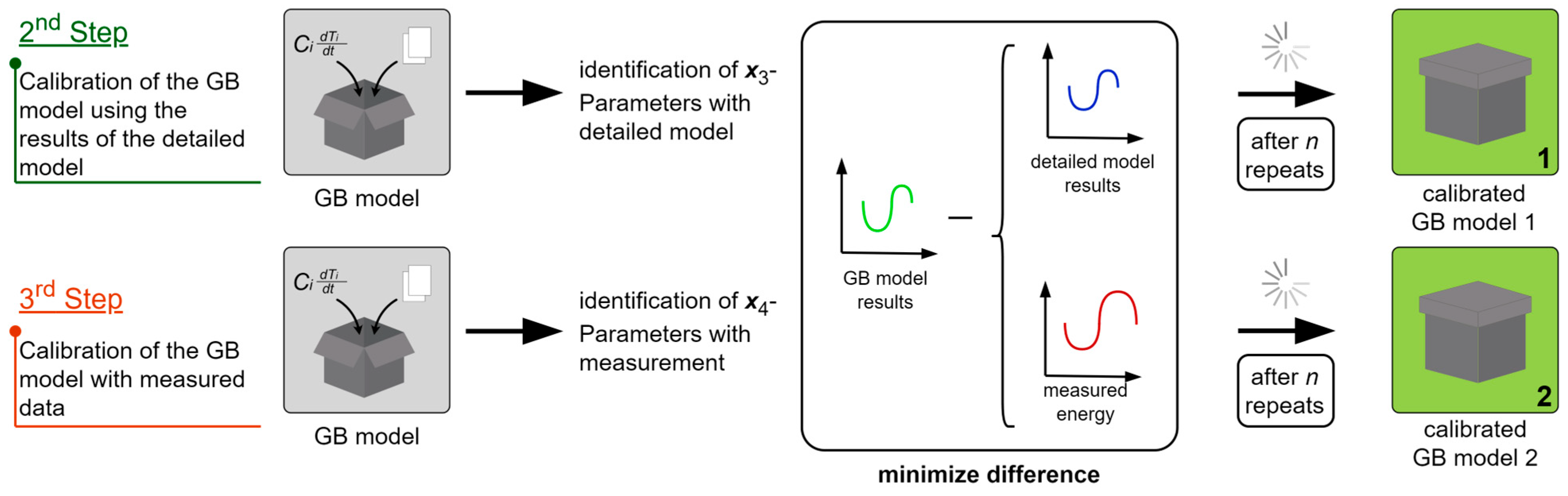
2.4.2. Step 2: Parameter Identification Based on Simulation Results

The parameters were adjusted by taking a multi-objective optimization approach (see Section 2.3.2), with five objective functions. The Root-Squared Error (RSE) was calculated for the heat flows and room temperature. The CV(RMSE) was used for monthly heating and cooling energy. By combining two different error metrics, the objective functions aim to achieve a balanced optimization that considers both the relative and absolute magnitudes of the errors. This approach helps to prevent the model from converging towards unrealistic solutions that may have low normalized errors but still have significant absolute deviations from the observed data and vice versa. A total of 1000 simulations were carried out. A parameter set that met the ASHRAE conditions for CV(RMSE) and NMBE was selected and resulted in a minimum RSE for the room temperature (35). The vector x3 describes the parameter set for each optimization run.
m i n x 3 R S E Q ˙ h e a t , Q ˙ ^ h e a t ,   R S E Q ˙ c o o l , Q ˙ ^ c o o l , R S E T i n , T ^ i n , C V ( R M S E ) h e a t , C V ( R M S E ) c o o l

2.4.3. Step 3: Parameter Identification Based on Measurements

The parameter identification process for the GB model was repeated for real-time measurement data for several reasons.
First, the detailed model was initially calibrated using monthly data, which effectively captured the typical behavior of the building but failed to represent its true dynamic time behavior. Detailed heat flow records of the considered building only recently became available. In addition, the building is currently controlled by an advanced energy management system that differs from the previous simple control strategy [51].
However, given these considerations, the parameter identification process was repeated using the measured data. This step was crucial for determining the suitability of the GB model for model predictive control applications. It ensured its adaptability to more dynamic and complex operational scenarios.
The parameters were adjusted by taking a multi-objective optimization approach (see Section 2.3.2), with three objectives functions. Compared to Equation (35), only a two-month period is analyzed here, which includes a heating, cooling, and transition period. As a result, the annual metrics of CV(RMSE) are not included. The Root-Squared Error (RSE) was calculated for the heat flows and the room temperature. A total of 1000 simulations were carried out. A specific set of parameters was chosen, which resulted in a minimum of the target function, giving a weight of 0.25 to the heat flows and 0.5 to the room air temperature. The vector x4 describes the parameter set for each optimization run.
m i n x 4 R S E Q ˙ h e a t , Q ˙ ^ h e a t ,   R S E Q ˙ c o o l , Q ˙ ^ c o o l , R S E T i n , T ^ i n

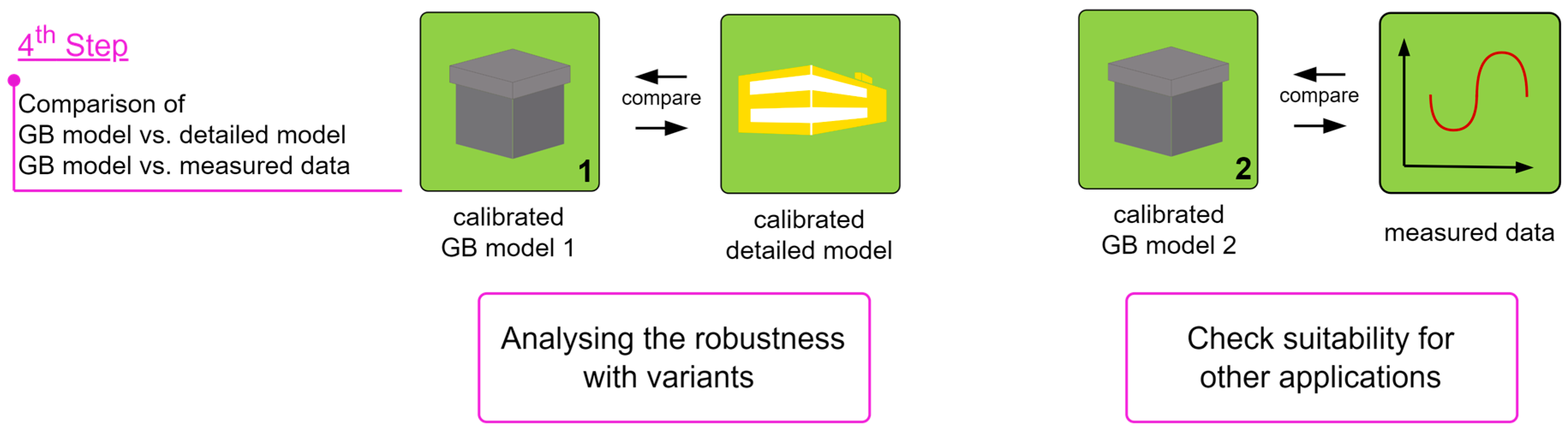
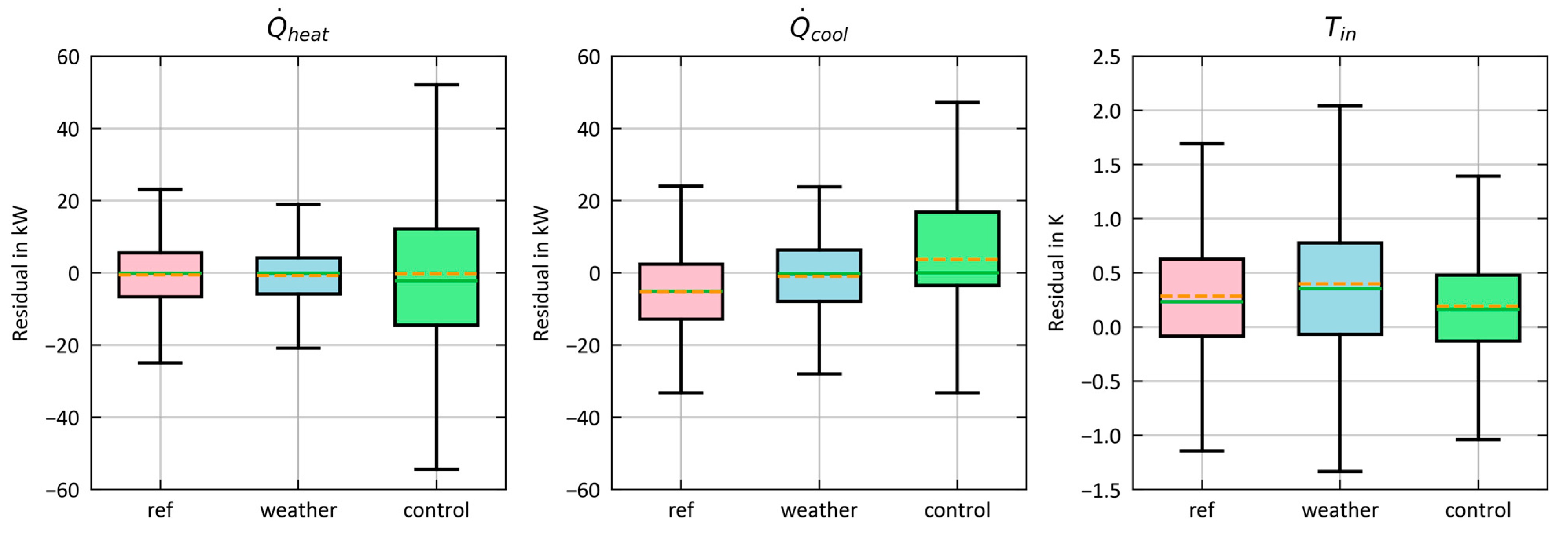
2.5. Step 4: Assessment of Robustness

To assess the robustness of the identified parameters and evaluate the generalizability of the GB model, three distinct simulation variants were analyzed:
  • Reference case: Involved simulations of both the GB1 and detailed models using 2021 weather data and the default control strategy with the identified parameters;
  • Weather case: Included simulations using 2019 weather data, while maintaining the parameters identified for the GB1 model;
  • Control case: Applied an alternative control strategy to the simulations, again maintaining the identified parameters.
These variations in weather data and control strategies are crucial for evaluating whether the parameter identification process has led to overfitting. If the GB model performs well across these different scenarios, it suggests that the identified parameters are robust and that the model has captured the underlying physical behavior of the system rather than simply memorizing the specific conditions of the calibration dataset.
Each variant involved a comparative analysis between the GB and detailed model under the respective conditions. In the control case, the floor valves were controlled via a PI controller. This controller adjusted the valve positions to maintain a minimum room temperature of 23 °C in the heating mode and a maximum of 26 °C in the cooling mode. The target temperature was an area-weighted average across all rooms. All valves were synchronized to respond to the same PI controller signal. The heating mode was activated when the one-hour moving average of the outdoor air temperature dropped below 14 °C, while the cooling mode was activated when the one-hour moving average of the outdoor temperature exceeded 21 °C.
Both the GB model and the detailed model include identical shading and window opening control to enable a comparison. However, they differ in the approach applied to the air quality strategies. One uses a CO2-based control, while the other uses a constant ACH when the room is occupied.
In addition, a final variant, the measurement case, was created to evaluate the model’s performance compared to the measured data and the model’s response to stochastic events. For this evaluation, the parameter identification process was repeated. This variant covered a two-month period, from 4 September 2023 to 4 November 2023, which was chosen due to the availability of additional heat flow and room air temperature measurement data. This period included cooling, heating, and transition periods. An average room temperature was calculated from measurements taken by 14 room air temperature sensors and compared to the GB2 model. We aimed to select the positions of the sensors so that they are representative of the building. A sensor was placed on each floor to measure the temperature in the circulation zone, which represents the central area on each floor. In addition, one office on the south side and the corner offices facing northeast and northwest were equipped. The remaining sensors were distributed to the large offices in the building. A floor plan with the positioning of the sensors is included in the Appendix A, Figure A1. The rationale behind the sensor positioning was to cover zones with different thermal loads (perimeter and core spaces) and occupancy densities.
The control strategy was derived from the measured data by converting mass flow rates into control signals, which were then fed into the GB2 model for simulation. The other control mechanisms are identical to those used in the other variants.

3. Model Evaluation

This section first presents the results of the parameter identification process of the detailed model, which has been validated by an experiment and by examining the monthly energy data for heating and cooling. Following the parameter identification, the focus shifts to the analysis of the deviations between the GB1 model and the detailed model. The discussion begins with a comprehensive analysis of the reference case. This is followed by a comparison analysis that was performed to analyze the heat flows and temperatures in different case scenarios. The purpose of this was to evaluate the robustness of the GB1 model under different conditions. The section concludes with the identification of the key parameters using the Morris method. The mean of the absolute values of the elementary effects is used in the analysis in this method. Finally, a comparison between the real-world measurements and the GB2 model’s simulation results for a two-month period is presented.

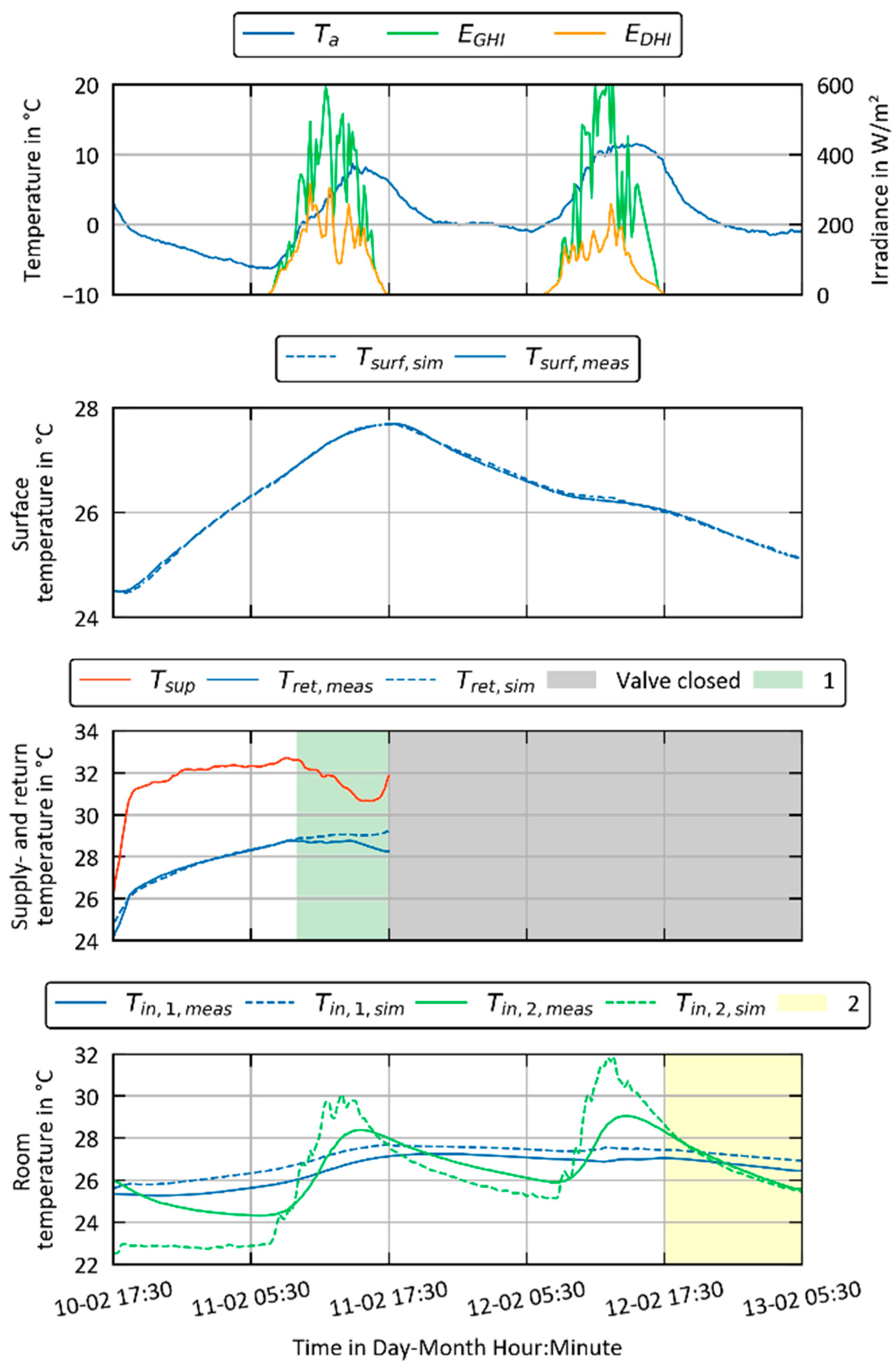
3.1. Detailed Model vs. Experimental Data

Figure 6 depicts the outside air temperature, global radiation, and diffuse radiation on the horizontal surface, simulated and measured average surface temperature of two rooms, and the supply and return temperatures of the thermally activated components of the whole building during the heating-up and cooling-down experiment (Stage 1.1, Figure 1). The room temperatures of two additional rooms are also plotted on this figure for further validation.
The surface temperatures observed in both the simulation and the measurements are in good agreement (Figure 6), as they are within the accuracy range of the built-in NTC sensors (±0.4 K). A decrease in the measured supply flow temperature occurred a few hours before the end of the heating-up phase, when a higher-level control deactivated the main pump supplying heat to the building, which is represented here by the green area and labeled with ‘1’. The pressure conditions in the real system changed due to the deactivation of the main supply pump. This resulted in a subsequent change in the mass flow. The simulation model does not take these changes into account. As a result, only the area prior to the green zone was used to optimize the return temperature. The grey area (valve closed) indicates that no mass flow is delivered to the thermally activated components within this time window.
The comparison between the simulated and measured indoor air temperatures was primarily used for visual cross-validation and not in the parameter identification process. The SHGC and the transparency of the shades, both of which influence heat gains, were identified later in the second stage. This resulted in deviations during the day. Therefore, the focus here is on periods without solar radiation, where the negative gradient of the simulated and measured values is expected to be similar. This is clearly the case in the yellow area marked with ‘2’. In the case of Room 1, the simulated room air temperature is similar to the measured temperature data, despite a noticeable offset.
In the second stage (Stage 1.2, Figure 1), the heat gain parameters, including internal loads, SHGC, and shading, were identified. This was conducted by using CV(RMSE) and NMBE, and by using monthly cooling and heating energy measurement data. Figure 7 illustrates the specific monthly energy demand and the metrics. All metrics meet the ASHRAE 14-2014 [37] requirements. The NMBE is within ±2.7% (with a threshold of 5% considered acceptable), and the CV(RMSE) values are within ±10% (with 15% being the required standard).

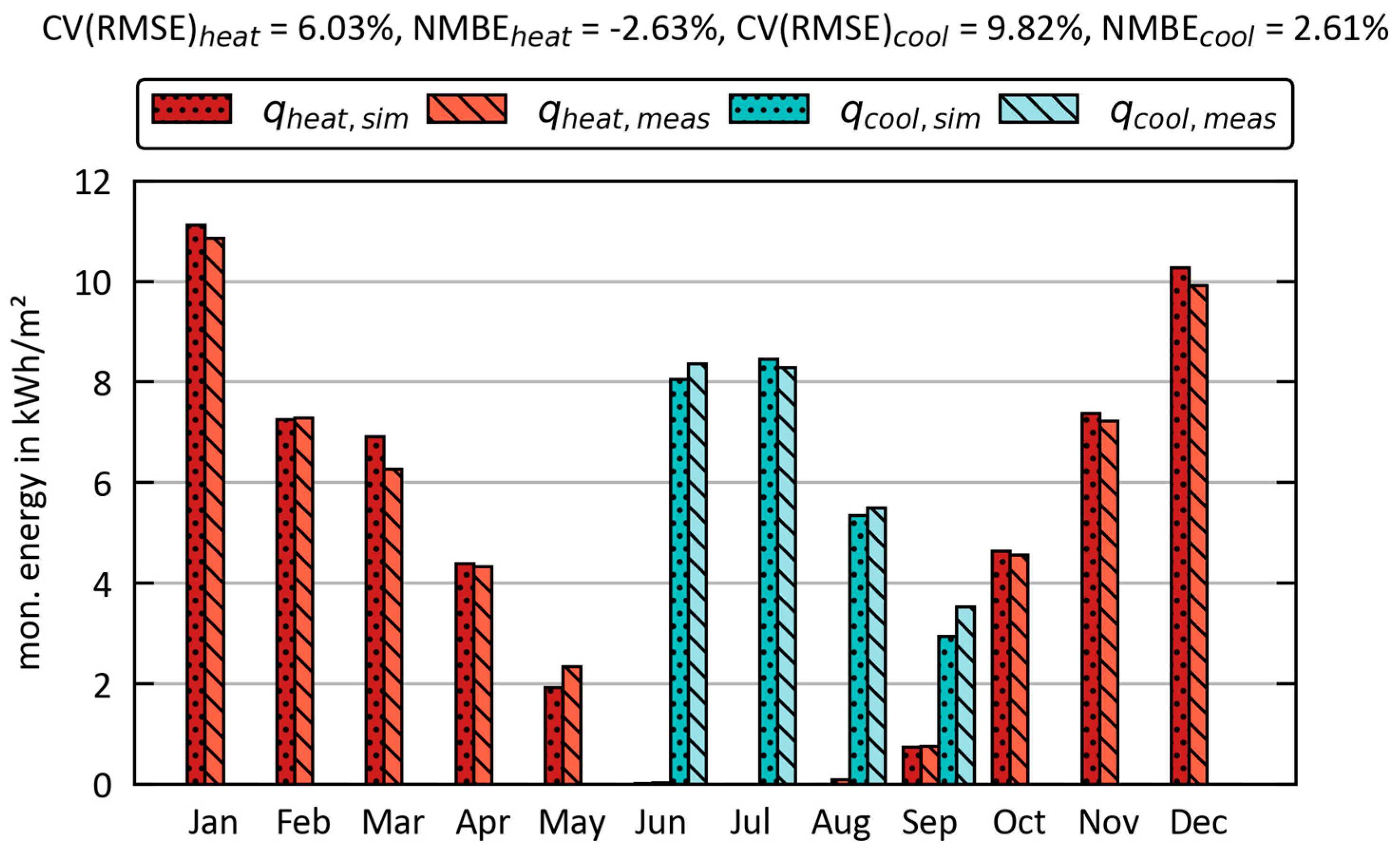
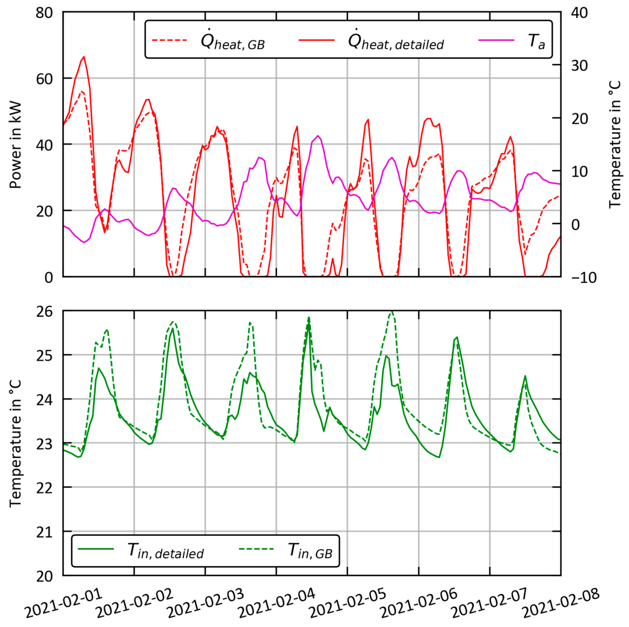
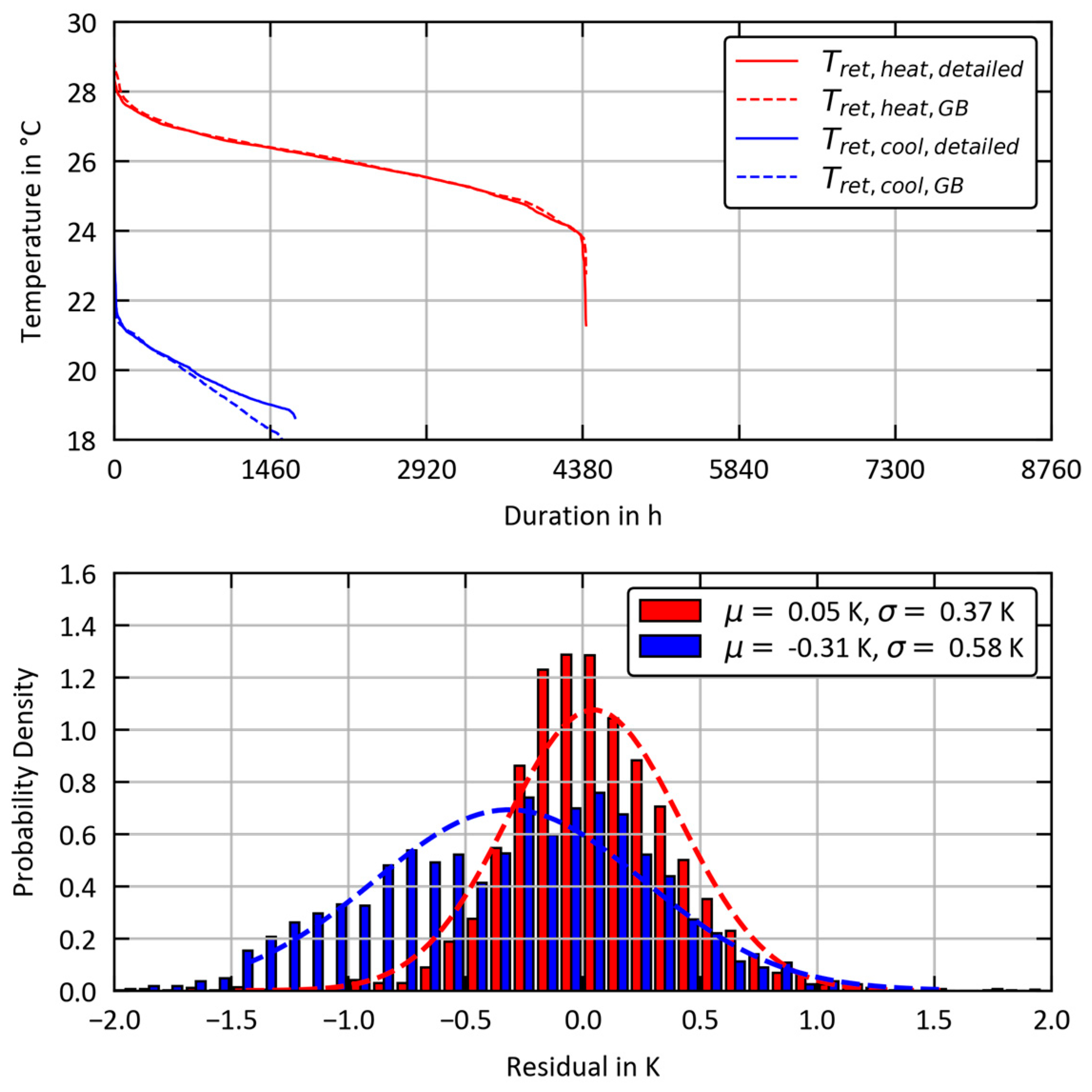
3.2. Grey-Box vs. Detailed Model

The simulated heating outputs for both the GB1 model and the detailed model during a typical week with a heating demand are shown in Figure 8. Similarly, Figure 9 shows the comparative results for a typical week with a cooling demand. The challenge in modeling the heat flows arises from the operational design of the system; it heats or cools based solely on the current outdoor air temperature, neglecting the room air temperatures, and only adjusts the supply temperature based on the outdoor air temperature (see Section 2.1). This operating characteristic results in relatively higher average indoor air temperatures in winter than in summer.
The agreement among the heat flows in the heating mode is particularly good in areas where both the detailed model and the GB1 model have the same room temperature. However, more significant deviations exceeding 10 kW are observed due to the faster cooldown of the room air node in the GB1 model. This results in an earlier increase in the heat flow in the heating mode. A contributing factor to this discrepancy is that no capacity is considered for the heat emission system in the GB1 model, which would otherwise help to dampen the fluctuations in the room air node temperature during the cooldown periods. This finding contrasts with the results reported in [32], where the authors claim that including additional mass for the heating and cooling system does not improve the accuracy of the model. Another possible explanation for these discrepancies is that the average internal and external gains during this period were underestimated in the GB1 model.
In the cooling mode, the heat flows seen in the models match closely, although a notable drawback is that the GB1 model tends to simulate higher room air temperatures than the detailed model. This results in an overestimation of heat flows by the GB1 model when the room air temperatures are the same in both models. Despite these discrepancies, the GB1 model replicates the system behavior simulated by the detailed model during the cooling and heating periods in an overall satisfactory way.
For a whole year simulation, the room air temperature deviation between the GB1 model and the detailed model shows a normal distribution. On average, the simulated room air temperature in the GB1 model is about 0.28 K higher than that of the detailed model, with a standard deviation of 0.62 K. Overall, the simulation results of the GB1 model match closely with those of the detailed model in terms of room temperature, as shown in Figure 10.
In the heating mode, the return temperatures of the GB1 model closely match those of the detailed model, with the residuals following a normal distribution. The mean deviation from the reference model is a mere 0.05 K, and a standard deviation of 0.37 K is seen, which falls within the accuracy range of the installed sensors. This agreement is attributed to the consistency of the heat flow at identical room air temperatures.
In the cooling period, the GB1 model results for the return temperature deviate notably from those of the detailed model, with a mean difference of −0.31 K and a standard deviation of 0.58 K. The primary cause for this deviation is the higher room air temperature simulated by the GB1 model at the same heat flow rate. In both systems, the mass flow is identical. Therefore, when the room temperatures are the same, the heat flow in the GB1 model is observed to be higher. This results in a lower return temperature in the GB1 model than in the detailed model, as illustrated in Figure 11.
Finally, the simulation times of the models were compared using the same hardware. The test system used for this comparison was an AMD Ryzen Threadripper PRO 5955WX running the Zen 3 architecture with 128 GB of DDR4 RAM. To perform a one-year simulation, the detailed model required 8229 s for the whole building, while the GB1 model with two capacities completed the simulation in 18 s. The maximal time step for the solver was 0.25 h. The minimum time step was not limited. These results indicate a 457-times higher computational efficiency when using the GB1 model.

3.3. Analysis of the Robustness

Simulations of the three variants defined in Section 2.5 (fourth step, Figure 3) are compared in this section for both the GB1 and the detailed model. For the variant ‘weather,’ the GB1 model shows robust behavior. In this scenario, the agreement between the detailed and GB1 model of the heat flows for heating and cooling is even better than in the reference case. The room air temperatures also show a higher deviation in both the mean and the interquartile range of the room air temperature compared to the reference case.
A different picture emerges for the third variant, ‘Control.’ Here, significant deviations are observed for the heat flows, as evidenced by the larger interquartile range in the data. Despite these deviations, it is noteworthy that the representation of room air temperatures in this third variant is more accurate than in the first two variants.
Despite the significant difference in the heat flow deviation in the heating period shown in Figure 12, the ‘control’ variant meets both the CV(RMSE) and NMBE metrics for monthly heating energy (Table 2). The underlying cause of this discrepancy is the earlier initiation and more uniform distribution of heat flow in the GB model, which results in its inability to accurately capture the peak load periods. In addition, the mass flow control in the GB1 model, which is governed by a proportional band and a minimum mass flow setting, also plays a role in these results. The cooling energy metrics in the control variant do not meet the specified requirements due to the higher simulated room air temperature of the GB1 model compared to the detailed model.
The analysis of the metrics in Table 2, which represent the deviations from the monthly simulated energy values from the detailed model, shows that the standards of ASHRAE Guideline 14-2014 [37] are almost met for the first two variants (‘reference’ and ‘weather’). In the ‘weather’ case, the NMBE slightly exceeds the standard by −0.108% in terms of heating energy. In the control case, the CV(RMSE) and NMBE for cooling are not met. To find out if this was due to the fact that the room air temperature in the GB1 model was consistently 0.28 K higher than in the detailed model, the setpoints were adjusted in an additional control variant, called ‘controladj’. This adjustment changes the heating setpoint from 23 °C to 23.28 °C and the cooling setpoint from 26 °C to 26.28 °C. After these set point adjustments were made, all metrics were observed to be in accordance with the mentioned standards (Table 2). This indicates that the model is not overfitted and can be reliably used for predictive simulations under a range of operating conditions.

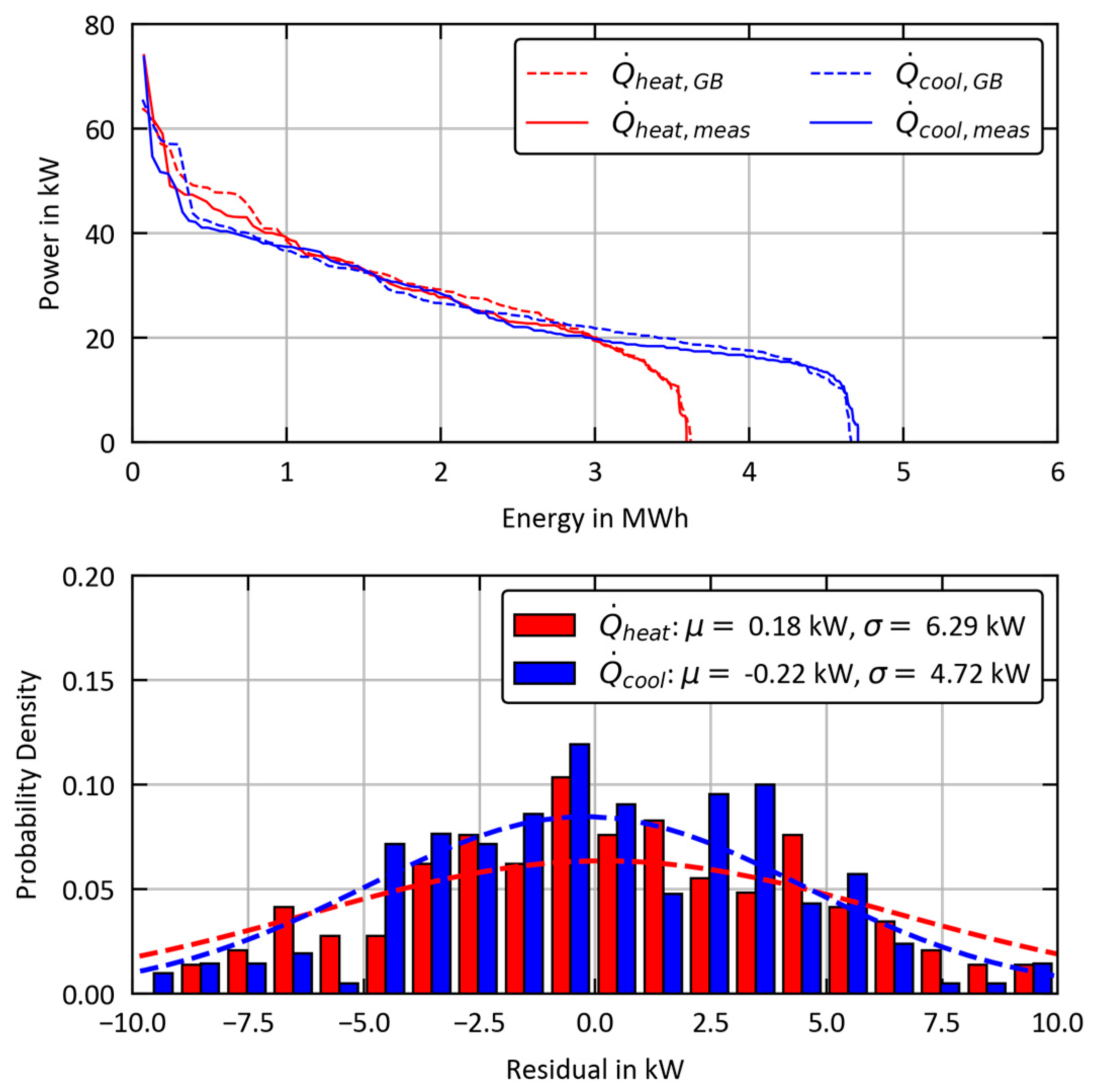
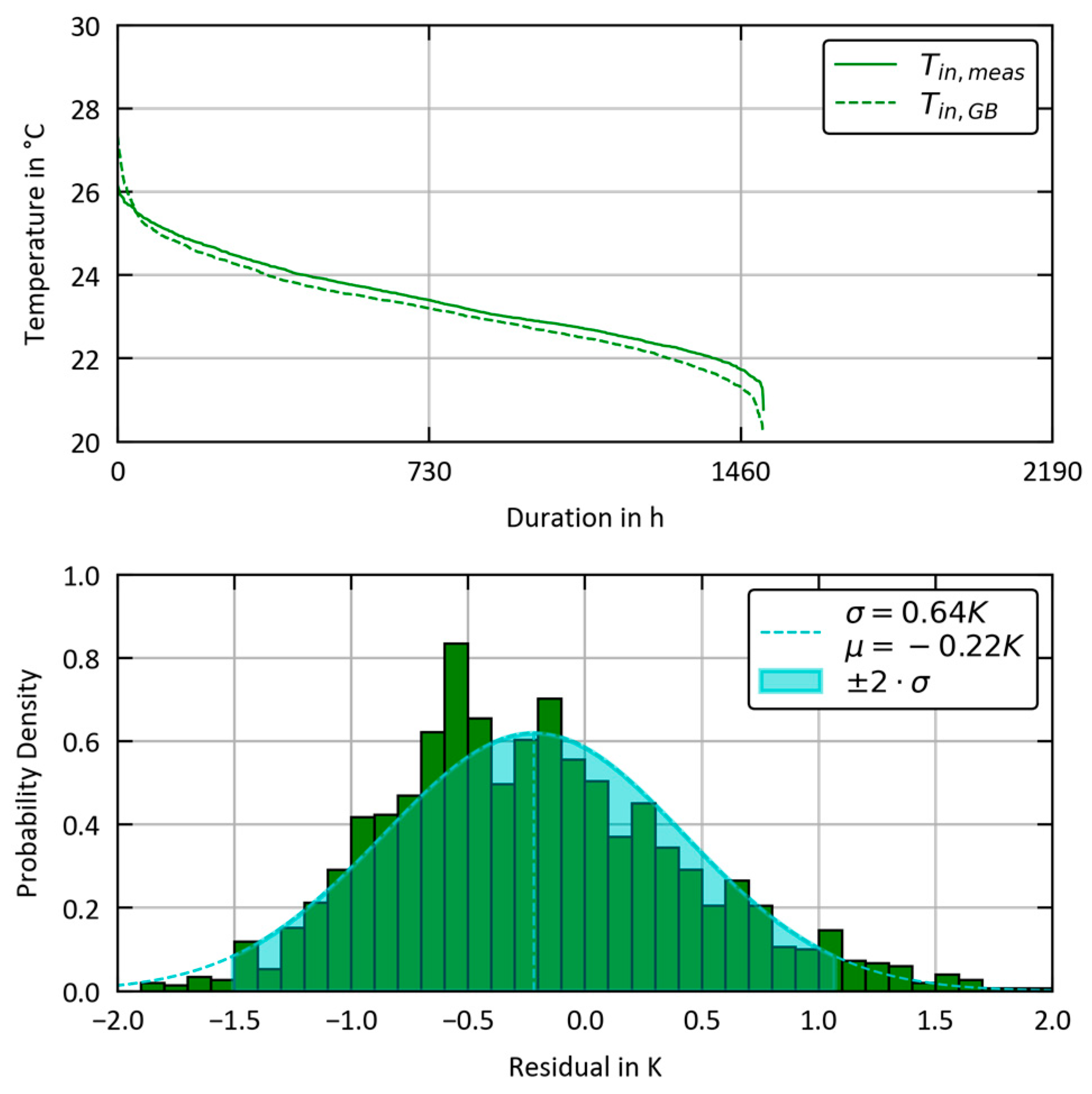
3.4. Grey Box vs. Measurement

When comparing the simulation results from the GB1 model for the considered two-month measurement period, and using the parameters derived from the detailed model, good agreement is shown for heating, but larger deviations are seen for periods with cooling. A possible reason for this discrepancy is the calibration of the detailed model with a heating-up experiment in winter without a corresponding cooling-down experiment in summer, and the unknown behavior of the occupants with shading and window control may affect the results.
In addition, the currently used advanced control mechanisms with an energy management system may contribute to these deviations. As shown in the robustness analysis, an alternative control strategy could lead to higher deviations in the heat flow simulation.
For the parameter identification process for the GB2 model, the parameters that have a higher order than six in the sensitivity analysis (Table 3) were not included in the process, and the values were taken from the final identification process with the detailed model from the GB1 model. The primary difference in the parameters identified for the GB2 model lies in reduced gains from radiation (fsol, shading) and reduced heat exchange with the environment (n50, U value). In addition, the NFA (farea) is greater. Due to the scaling effect of the NFA on the entire system, a larger farea compensates for the lower radiation gains and heat exchange with the environment.
The energy demand predicted by the GB2 model closely matches the measured data, with a deviation of 0.2% seen for cooling and 1.7% for heating energy, as shown in Figure 13. The discrepancy between the simulated and measured heat flows mirrors the behavior observed in the comparison between the GB2 model and the detailed model. For both heating and cooling, the residuals of the heat flows follow a normal distribution, with a mean deviation of 0.18 kW (σ = 6.29 kW) for heating and −0.22 kW (σ = 6.29 kW) for cooling.
For the two-month simulation period, the residuals between the GB2 model and the actual measurements show a normal distribution for room air temperatures (as shown in Figure 14) and return temperatures (as shown in Figure 15). In contrast to the comparison with the detailed model, where the GB1 model typically shows higher room air temperatures, the GB2 model in this case shows a slightly lower temperature on average, with a difference of −0.22 K from the measured values. Similarly, the comparison between the simulated return temperatures for heating and cooling and the actual measurements reveals similar behavior to the comparison between the GB1 model and the detailed model.
Overall, the comparison of the GB2 model with the actual measured values indicates that the deviation falls within the same order of magnitude as the deviation observed when comparing the GB1 model with the detailed model. This consistency not only underscores the potential of the GB model as a viable alternative to a detailed model but also highlights its suitability as a basis for model predictive control applications.

3.5. Sensitivity Analysis

The function that is used in the Morris method is the NMBE for heating and cooling energy. For a more complete understanding of the method, see [35]. The parameter ranges are set to ± 25% of the identified values (see Section 2.4.2) to define their limits for the Morris method. The parameters that were used and their order are listed in Table 3. The parameter range is subdivided into p = 4 levels, which led to accurate results according to [52]. As suggested in [35], 10 trajectories were recommended. Additionally, a comprehensive convergence analysis spanning from 1 to 300 trajectories was conducted to ensure the reliability and stability of the results (Figure A2).
The analysis of the most influential parameters in the developed model shows that the specific masses of the interior (Cin) and exterior (Ce) have a minimal impact on the NMBE metrics. The most important parameter is the area factor (farea), since it scales the NFA and consequently affects all the specific parameters. The importance of each parameter is listed in Table 3.
Parameters that are critical for both heating and cooling are those that affect internal and external gains, such as the internal gain factor (internal) and the solar factor (fsol). The U-value and the factor fa,α, which affect the equivalent outdoor temperature, are also critical.
Figure A2 shows the convergence analysis of the Morris method over a range of 1 to 300 trajectories. The analysis shows that convergence is reached at approximately the 200th trajectory. The order, which is also shown in Table 3, is reversed in Figure A2. The parameters are of approximately equal importance from order 6 and on.

4. Conclusions and Outlook

This paper presents a non-linear GB model with an integrated water-based heating and cooling system, based on physical principles, that can be used for efficient and accurate thermal building simulations. A detailed physical model (38 thermal zones) of a university building with a heat emission system based on concrete core activation was created and validated with heating-up and cooling-down experiments to provide a meaningful comparison between real, measured results and results from the simulation model. Measurement data was extracted from an IoT system, including supply and return, surface, and indoor air temperatures. Moreover, the GB model’s accuracy and performance were evaluated against real-world measurement data, including heat flows.

4.1. Scientific Contributions and Practical Implications

The paper describes the development and comprehensive verification of a non-linear GB model with a layered calibration workflow. In the chosen workflow, the GB model was first calibrated with data from a detailed white-box model, due to a lack of measurement data from the considered building. In a second step, the GB model was calibrated with available measured data from a two-month period.
The GB model accurately reflects the dynamics of the detailed model and the measurement, particularly when comparing the room and return temperatures. Despite challenges related to real-time heat flow accuracy, its efficiency is characterized by a 457-fold increase in the simulation speed compared to that of the detailed model, while reliable metrics are maintained under various conditions. The key highlights include:
  • Extensive validation and integration of a water-based heat emission system: The GB model includes a water-based heating and cooling system capable of predicting thermal power and return temperatures with sufficient accuracy. Its development involved a thorough validation process, comparing it to a detailed physical model and real-world measurement data;
  • Minimal input requirements: A notable feature of the GB model is that it requires only a few input parameters for effective parameterization. This aspect enhances its usability and accessibility to a wide range of users;
  • Demonstration of the optimization process: An exemplary optimization process to identify the model parameters was demonstrated, including a sensitivity analysis, showing the practical application and versatility in real-world scenarios.
The GB model presented in this paper is flexible, and it should be able to support two primary use cases, both of which remain to be tested in future work:
  • Urban building energy modeling (UBEM): The model could be used in UBEM scenarios, where parameterization requires only basic system design conditions and monthly measured values for heating and/or cooling demand. This makes it a suitable replacement for detailed models, which are much more time-consuming and for which, usually, not all necessary data is available for many buildings. Parameterization with monthly data leads to a loss of accuracy in comparison. However, for studies involving a large number of buildings, this should be manageable, as the energy demand is considered correctly. Additionally, the heat dissipation system and dynamic behavior are taken into account;
  • Demand-side management and model predictive control: The model could also be applicable to the demand-side management of buildings and could serve as a foundational element for model predictive control systems, enabling the more accurate and responsive control of building energy systems. For these applications, additional measurement data are required for effective model training. These include data such as a time series of the average indoor air temperature and heating/cooling heat flows. These data can come either from a more detailed model or from measurements.

4.2. Study Limitations and Future Research

The GB model shows good agreement with the detailed physical building model and with the measurements for the considered scenarios. However, it has its limitations. Primarily, it is a one-zone model and cannot replace a detailed physical simulation model with multiple zones and complex air-handling units. In larger buildings, particularly those with different types of use, e.g., residential and office use, heating and cooling requirements can occur simultaneously in different zones, especially during the transitional period. Of course, a one-zone model cannot take this into account. In addition, the model exhibited inaccuracies in real-time heat flow simulation, which is partly due to not taking into account the thermal mass capacity in the heat emission system.
Future work will focus on the application and testing of the model to different kinds and sizes of buildings and the use cases mentioned above. Additionally, the effects of direct normal radiation and integrating the capacity of the heat emission system, which should be especially beneficial for concrete core activation as used in this work, will be explored. Furthermore, improving the heat transfer representation with long-wavelength radiation and experimenting with alternative optimization methods will be considered, as the AutoMOO algorithm used in this work is in the beta-testing phase in IDA ICE Beta 28. The next phase of the research will involve integrating the models into a neighborhood simulation at Graz University of Technology. In this step, different centralized and decentralized cooling configurations will be tested to increase the practical applicability and real-world relevance of the model.
Thermal building simulation is an important tool on the way to optimizing energy efficiency and sustainability. The presented model contributes to a simplified creation of building models and time- and resource-saving thermal building simulations.

Author Contributions

M.M.: Conceptualization, Methodology, Formal analysis, Data curation, Software, Investigation, Validation, Visualization, Writing—original draft. A.H.: Writing—review and editing. R.H.: Conceptualization, Project administration, Writing—review & editing. H.E.: Conceptualization, Writing—review and editing. T.M.: Funding acquisition, Project administration, Writing—review and editing. V.K.: Data curation, Writing—review and editing. M.G.: Funding acquisition, Writing—review and editing. C.H.: Writing—review and editing, Supervision. All authors have read and agreed to the published version of the manuscript.

Funding

This research was funded by the Österreichische Forschungsförderungsgesellschaft mbH (FFG), within the project “COOL-QUARTER-PLUS”, grant number 879460 within the program “City of Tomorrow”, and by the Austrian State of Styria, grant number 1406, within the program “Zukunftsfonds Steiermark, 14th call NEXT GREEN TECH”. The APC was funded by Graz University of Technology.

Data Availability Statement

Data will be made available on request.

Acknowledgments

This work significantly builds upon a foundational simulation model developed by Peter Nageler (EQUA). Supported by TU Graz Open Access Publishing Fund.

Conflicts of Interest

Valentin Kaisermayer and Markus Gölles are affiliated with BEST—Bioenergy and Sustainable Technologies GmbH. The remaining authors declare that they have no known competing financial interests or personal relationships that could have appeared to influence the work reported in this paper.

Nomenclature

Variables and parametersTinRoom air temperature, °C
AArea, m2Tin, setRoom air set temperature, °C
ACHAir exchange rate, 1/hTretReturn water temperature, °C
albedoReflection coefficient from the environmentTsupSupply/forward water temperature, °C
cSimultaneity factor of direct normal radiationUHeat transfer coefficient, W/(m2K)
CeHeat capacity of the exterior/thermally active storage mass, J/KVAir volume of the building, m3
CinHeat capacity of the indoor air, J/KvVectorial wind speed, m/s
cp,aSpecific heat capacity of the air, J/(kgK)zHeight, m
Cp,vMean pressure coefficient over the buildingafAbsorption coefficient of the outer wall
cp,wSpecific heat capacity of water, J/(kgK)ΔpPressure difference between inside and outside, Pa
EDHISpecific diffuse irradiance on the horizontal surface, W/m2ϑTemperature difference between fluid and room air temperature, K
EDNISpecific direct normal irradiance, W/m2ϑ0Temperature difference between supply water and room air temperature, K
EGHISpecific global irradiance on the horizontal surface, W/m2ϑlogLogarithmic mean temperature difference between water and room air temperature, K
fa,αRatio of af and haΘmDimensionless mean temperature
fareaRatio of net floor area and gross floor areaκCoefficient of performance
feffFactor for the effectiveness of air exchange caused by pressure differenceµi*The absolute mean of elementary effects
ρaMass density of the air, kg/m3
fshapeRatio of vertical and horizontal surface areaΦSun position: azimuth, °
fsignalOverall control signal for heating or coolingIndices
fsolSolar factorbBuoyancy effect
fvalveControl signal for mass flow controlbuiBuilding
haHeat transfer coefficient between outer wall and environment, W/(m2K)horHorizontal
hconvConvective heat transfer coefficient, W/(m2K)nomNominal/design conditions
kHeat transfer coefficient, W/(m2K)occOccupied
m ˙ Mass flow of the water-based radiator system, kg/ssurfSurface
nHeater exponentverVertical
n50Air exchange rate at a pressure difference of 50 Pa, 1/hwinWindow ventilation
nxAir exchange rate caused by a pressure difference, 1/hAbbreviations
paAir pressure, PaAutoMOOAutomatic Multi-Objective Optimization
pbandProportional band of the mass flow control, KBEMBuilding energy modeling
Q ˙ h e a t Heat flow from the heating system to the room node, WBIMBuilding Information Modeling
Q ˙ A C H Heat flow due to air exchange, WCCapacities
Q ˙ c o o l Heat flow from the room node to the cooling system, WCV(RMSE)Coefficient of Variation of the Root-Mean-Square Error
Q ˙ i n f Heat flow due to pressure differences, WGBGrey-box
Q ˙ i n t Heat flow due to internal gains, WGFAGross floor area
Q ˙ s o l Heat flow due to solar radiation, WGHGGreenhouse gas
RaGas constant of the air, J/(kgK)IFCIndustry Foundation Classes
Re,aHeat transfer resistance between the thermally activated storage mass and the equivalent outdoor air temperature, K/WIoTInternet-of-things
Rin,aHeat transfer resistance between the outdoor temperature and the room air temperature, K/WNFANet floor area
Rin,eHeat transfer resistance between the two nodes, K/WNMBENormalized-Mean-Bias Error
sRadiative fraction of heat transfer of the heating and cooling systemRResistances
TaOutdoor air temperature, °CRSERoot-Square Error
Ta,eqEquivalent outdoor air temperature, °CSHGCSolar heat gain coefficient, g-value
TeThermally active storage mass temperature, °CUBEMUrban Building Energy Simulation Models

Appendix A

Appendix A.1. Detailed Model Boundary Conditions

Table A1. Allocation of the internal loads from SIA 2024:2021 to DIN 277.
Utilization Number
DIN 277SIA 2024
NF7.112.06
NF1.24.02
NF2.13.01
NF2.33.03
NF3.39.03
NF3.812.05
NF4.112.04
NF4.212.04
NF5.24.01
NF5.44.03
TF8.412.04
TF8.912.04
VF9.112.01
VF9.212.03
VF9.312.04
VF9.912.01

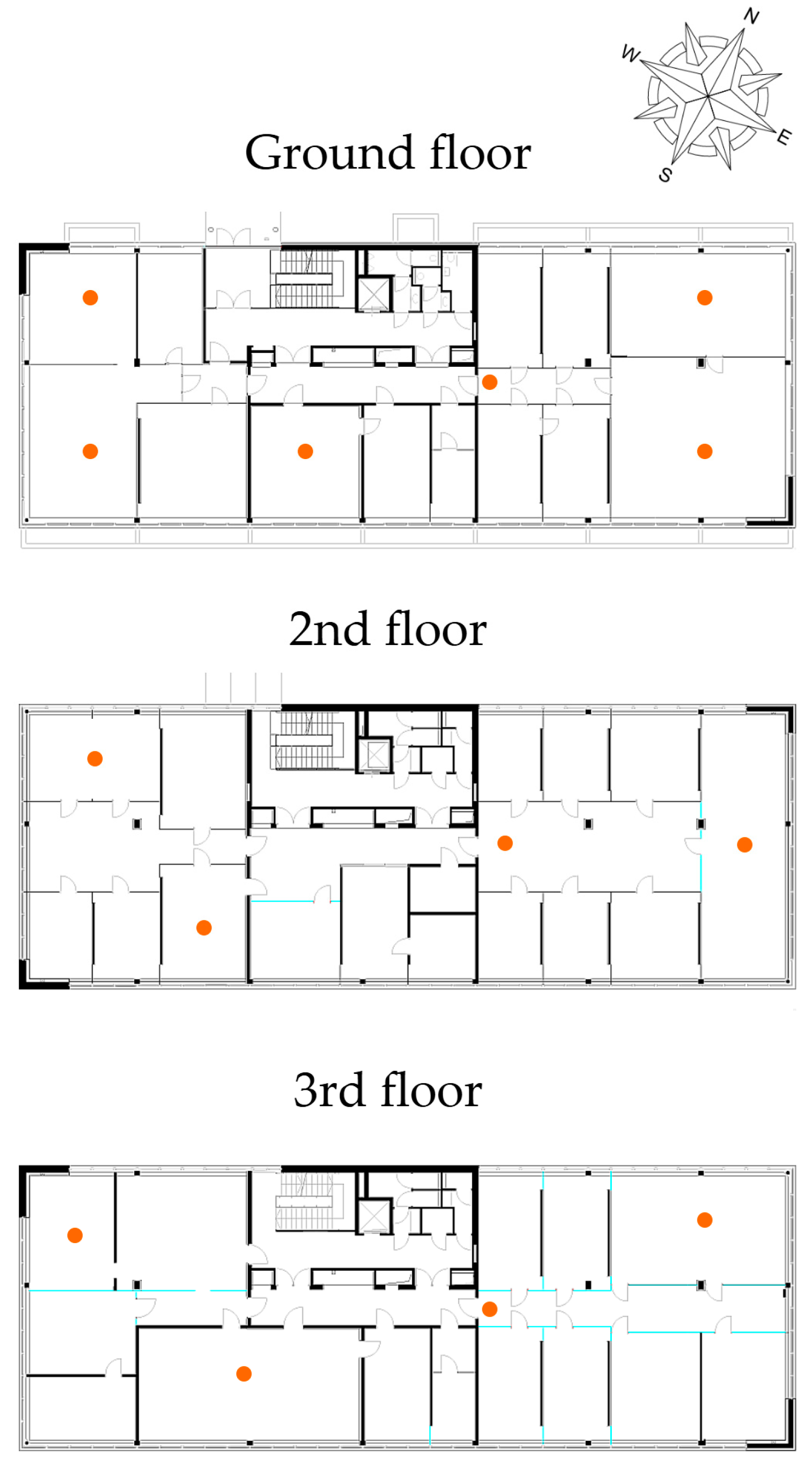
Appendix A.2. Sensor Positioning

Figure A1. Positioning of temperature sensors across the three floors of the building.
Buildings 15 01959 g0a1

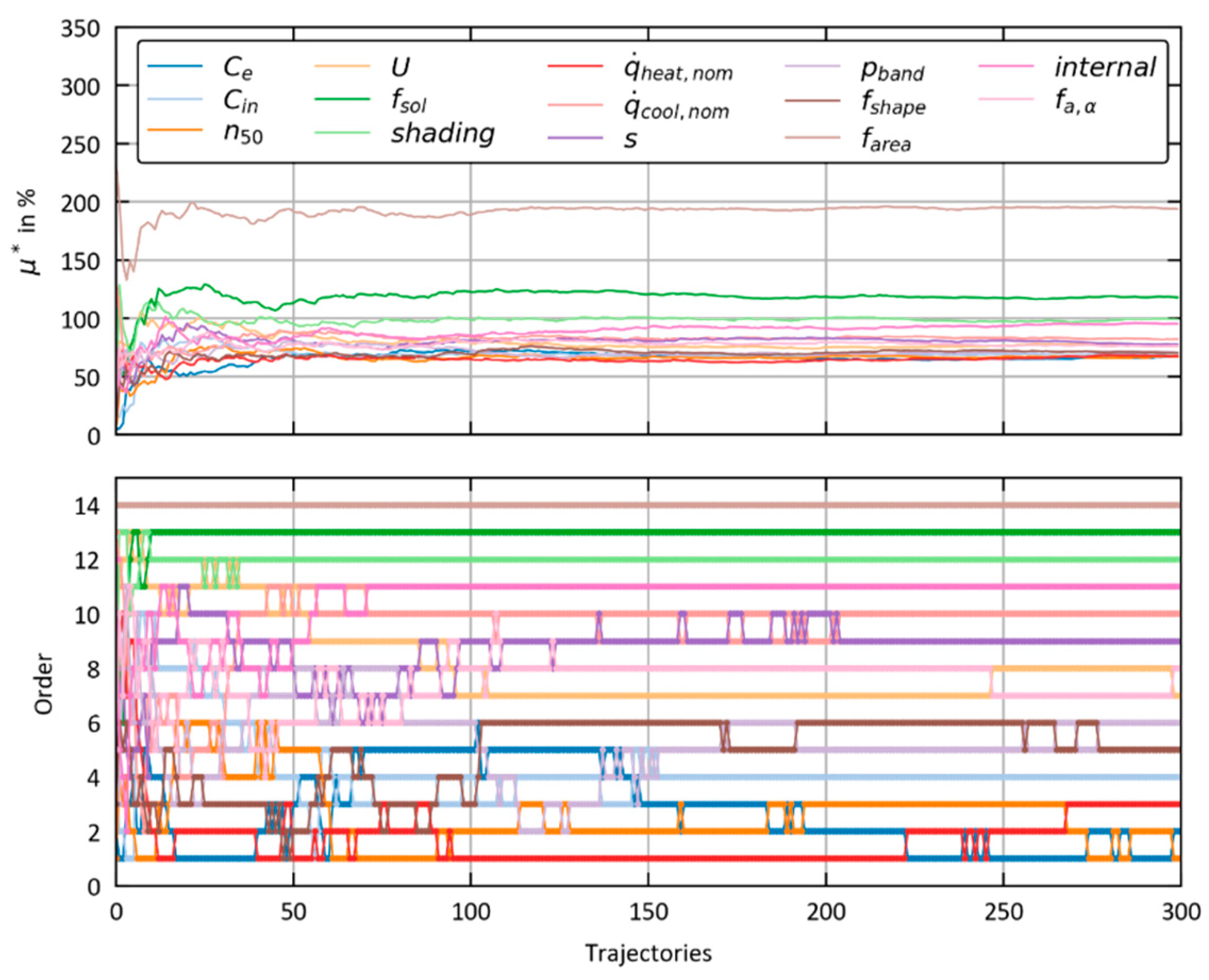
Appendix A.3. Morris Convergence Analysis

Figure A2. The evolution of mean elementary effect (µ*) on the NMBEcool for all parameters (xi) as a function of the number of trajectories. The lower section indicates the order of importance of the parameters, with higher order numbers indicating greater importance.
Buildings 15 01959 g0a2

References

  1. Nejat, P.; Jomehzadeh, F.; Taheri, M.M.; Gohari, M.; Majid, M.Z.A. A global review of energy consumption, CO2 emissions and policy in the residential sector (with an overview of the top ten CO2 emitting countries). Renew. Sustain. Energy Rev. 2015, 43, 843–862. [Google Scholar] [CrossRef]
  2. IPCC Working Group I. IPCC Sixth Assessment Report, Climate Change 2021: The Physical Science Basis; The Intergovernmental Panel on Climate Change (IPCC): Geneva, Switzerland, 2021. [Google Scholar]
  3. Yin, R.; Xu, P.; Piette, M.A.; Kiliccote, S. Study on Auto-DR and pre-cooling of commercial buildings with thermal mass in California. Energy Build. 2010, 42, 967–975. [Google Scholar] [CrossRef]
  4. Zhou, Q.; Wang, S.; Xu, X.; Xiao, F. A grey-box model of next-day building thermal load prediction for energy-efficient control. Int. J. Energy Res. 2008, 32, 1418–1431. [Google Scholar] [CrossRef]
  5. Lee, K.; Braun, J.E. Model-based demand-limiting control of building thermal mass. Build. Environ. 2008, 43, 1633–1646. [Google Scholar] [CrossRef]
  6. Mirakhorli, A.; Dong, B. Model predictive control for building loads connected with a residential distribution grid. Appl. Energy 2018, 230, 627–642. [Google Scholar] [CrossRef]
  7. Fabre, A.; Thomas, R.; Duplessis, B.; Tran, C.-T.; Stabat, P. Dynamic modeling for evaluation of triple-pipe configuration potential in geothermal district heating networks. Energy Convers. Manag. 2018, 173, 461–469. [Google Scholar] [CrossRef]
  8. Kim, E.-J.; Plessis, G.; Hubert, J.-L.; Roux, J.-J. Urban energy simulation: Simplification and reduction of building envelope models. Energy Build. 2014, 84, 193–202. [Google Scholar] [CrossRef]
  9. Heidarinejad, M.; Mattise, N.; Dahlhausen, M.; Sharma, K.; Benne, K.; Macumber, D.; Brackney, L.; Srebric, J. Demonstration of reduced-order urban scale building energy models. Energy Build. 2017, 156, 17–28. [Google Scholar] [CrossRef]
  10. Edtmayer, H.; Nageler, P.; Heimrath, R.; Mach, T.; Hochenauer, C. Investigation on sector coupling potentials of a 5th generation district heating and cooling network. Energy 2021, 230, 120836. [Google Scholar] [CrossRef]
  11. Drgoňa, J.; Arroyo, J.; Figueroa, I.C.; Blum, D.; Arendt, K.; Kim, D.; Ollé, E.P.; Oravec, J.; Wetter, M.; Vrabie, D.L.; et al. All you need to know about model predictive control for buildings. Annu. Rev. Control 2020, 50, 190–232. [Google Scholar] [CrossRef]
  12. American Society of Heating, Refrigerating and Air Conditioning Engineers, Inc. ASHRAE Handbook-Fundamentals; D&R International, Ltd.: McLean, VA, USA, 2013. [Google Scholar]
  13. Coakley, D.; Raftery, P.; Keane, M. A review of methods to match building energy simulation models to measured data. Renew. Sustain. Energy Rev. 2014, 37, 123–141. [Google Scholar] [CrossRef]
  14. Shahcheraghian, A.; Madani, H.; Ilinca, A. From White to Black-Box Models: A Review of Simulation Tools for Building Energy Management and Their Application in Consulting Practices. Energies 2024, 17, 376. [Google Scholar] [CrossRef]
  15. Zhang, Y.; O’Neill, Z.; Dong, B.; Augenbroe, G. Comparisons of inverse modeling approaches for predicting building energy performance. Build. Environ. 2015, 86, 177–190. [Google Scholar] [CrossRef]
  16. Dong, B.; Cao, C.; Lee, S.E. Applying support vector machines to predict building energy consumption in tropical region. Energy Build. 2005, 37, 545–553. [Google Scholar] [CrossRef]
  17. Berthou, T.; Stabat, P.; Salvazet, R.; Marchio, D. Comparaison de Modèles Linéaires Inverses Pour la Mise en Place de Stratégies D’effacement. In Proceedings of the Rencontres AUGC-IBPSA, Chambéry, France, 6–8 June 2012. [Google Scholar]
  18. Attoue, N.; Shahrour, I.; Mroueh, H.; Younes, R. Determination of the Optimal Order of Grey-Box Models for Short-Time Prediction of Buildings’ Thermal Behavior. Buildings 2019, 9, 198. [Google Scholar] [CrossRef]
  19. Bacher, P.; Madsen, H. Identifying suitable models for the heat dynamics of buildings. Energy Build. 2011, 43, 1511–1522. [Google Scholar] [CrossRef]
  20. Brastein, O.M.; Perera, D.; Pfeifer, C.; Skeie, N.-O. Parameter estimation for grey-box models of building thermal behaviour. Energy Build. 2018, 169, 58–68. [Google Scholar] [CrossRef]
  21. Ghosh, S.; Reece, S.; Rogers, A.; Roberts, S.; Malibari, A.; Jennings, N.R. Modeling the Thermal Dynamics of Buildings. ACM Trans. Intell. Syst. Technol. 2015, 6, 1–27. [Google Scholar] [CrossRef]
  22. Arroyo, J.; Spiessens, F.; Helsen, L. Identification of multi-zone grey-box building models for use in model predictive control. J. Build. Perform. Simul. 2020, 13, 472–486. [Google Scholar] [CrossRef]
  23. González, V.G.; Ruiz, G.R.; Bandera, C.F. Empirical and Comparative Validation for a Building Energy Model Calibration Methodology. Sensors 2020, 20, 5003. [Google Scholar] [CrossRef]
  24. Yousaf, S.; Bradshaw, C.R.; Kamalapurkar, R.; San, O. A gray-box model for unitary air conditioners developed with symbolic regression. Int. J. Refrig. 2024, 168, 696–707. [Google Scholar] [CrossRef]
  25. Reynders, G.; Diriken, J.; Saelens, D. Quality of grey-box models and identified parameters as function of the accuracy of input and observation signals. Energy Build. 2014, 82, 263–274. [Google Scholar] [CrossRef]
  26. Afram, A.; Janabi-Sharifi, F. Gray-box modeling and validation of residential HVAC system for control system design. Appl. Energy 2015, 137, 134–150. [Google Scholar] [CrossRef]
  27. Hu, J.; Karava, P. A state-space modeling approach and multi-level optimization algorithm for predictive control of multi-zone buildings with mixed-mode cooling. Build. Environ. 2014, 80, 259–273. [Google Scholar] [CrossRef]
  28. Li, Y.; O’Neill, Z.; Zhang, L.; Chen, J.; Im, P.; DeGraw, J. Grey-box modeling and application for building energy simulations—A critical review. Renew. Sustain. Energy Rev. 2021, 146, 111174. [Google Scholar] [CrossRef]
  29. Kramer, R.; van Schijndel, J.; Schellen, H. Inverse modeling of simplified hygrothermal building models to predict and characterize indoor climates. Build. Environ. 2013, 68, 87–99. [Google Scholar] [CrossRef]
  30. Afshari, A.; Liu, N. Inverse modeling of the urban energy system using hourly electricity demand and weather measurements, Part 2: Gray-box model. Energy Build. 2017, 157, 139–156. [Google Scholar] [CrossRef]
  31. Thilker, C.A.; Bacher, P.; Bergsteinsson, H.G.; Junker, R.G.; Cali, D.; Madsen, H. Non-linear grey-box modelling for heat dynamics of buildings. Energy Build. 2021, 252, 111457. [Google Scholar] [CrossRef]
  32. Harb, H.; Boyanov, N.; Hernandez, L.; Streblow, R.; Müller, D. Development and validation of grey-box models for forecasting the thermal response of occupied buildings. Energy Build. 2016, 117, 199–207. [Google Scholar] [CrossRef]
  33. Berthou, T.; Stabat, P.; Salvazet, R.; Marchio, D. Development and validation of a gray box model to predict thermal behavior of occupied office buildings. Energy Build. 2014, 74, 91–100. [Google Scholar] [CrossRef]
  34. EQUA Simulation AB. IDA ICE 5 Beta 28-Simulation Software|EQUA. Available online: https://www.equa.se/de/ida-ice (accessed on 11 November 2023).
  35. Morris, M.D. Factorial Sampling Plans for Preliminary Computational Experiments. Technometrics 1991, 33, 161–174. [Google Scholar] [CrossRef]
  36. Herman, J.; Usher, W. SALib: An open-source Python library for Sensitivity Analysis. J. Open Source Softw. 2017, 2, 97. [Google Scholar] [CrossRef]
  37. ASHRAE. ASHRAE Guideline 14-2014: Measurement of Energy, Demand and Water Savings; American Society of Heating, Refrigerating and Air-Conditioning Engineers: Atlanta, GA, USA, 2014. [Google Scholar]
  38. DIN 277-1:2021-08; Areas and volumes in building construction—Part 1: Terms, definitions and calculation principles. Deutsches Institut für Normung (DIN): Berlin, Germany, 2021.
  39. SIA 2024:2021; Raumnutzungsdaten für die Energie- und Gebäudetechnik. Schweizerischer Ingenieur- und Architektenverein (SIA): Zürich, Switzerland, 2021.
  40. B 8110-7; Wärmeschutz im Hochbau: Teil 7: Tabellierte wärmeschutztechnische Bemessungswerte. Austrian Standards International: Wien, Austria, 2013.
  41. Mörth, M. Analyse und Transformation von Quartiers-Energiesystemen am Beispiel Innovation District Inffeld. MSc, Institut für Wärmetechnik, Technischen Universität Graz, Graz, 2022. Available online: https://online.tugraz.at/tug_online/wbAbs.showThesis?pThesisNr=76874&pOrgNr=2267# (accessed on 9 April 2024).
  42. Bundesanstalt für Geologie. Geophysik, Klimatologie und Meteorologie—GeoSphere. Available online: https://data.hub.geosphere.at/ (accessed on 19 November 2023).
  43. Gouda, M.M.; Danaher, S.; Underwood, C.P. Building thermal model reduction using nonlinear constrained optimization. Build. Environ. 2002, 37, 1255–1265. [Google Scholar] [CrossRef]
  44. Vivian, J.; Zarrella, A.; Emmi, G.; de Carli, M. An evaluation of the suitability of lumped-capacitance models in calculating energy needs and thermal behaviour of buildings. Energy Build. 2017, 150, 447–465. [Google Scholar] [CrossRef]
  45. Loutzenhiser, P.G.; Manz, H.; Felsmann, C.; Strachan, P.A.; Frank, T.; Maxwell, G.M. Empirical validation of models to compute solar irradiance on inclined surfaces for building energy simulation. Sol. Energy 2007, 81, 254–267. [Google Scholar] [CrossRef]
  46. EN ISO 52016-1; Energetische Bewertung von Gebäuden—Berechnung des Energiebedarfs für Heizung und Kühlung, Innentemperaturen Sowie der Heiz- und Kühllast in Einem Gebäude oder Einer Gebäudezone: Teil 1: Berechnungsverfahren. Austrian Standards International: Vienna, Austria, 2018.
  47. Großmann, H.; Böttcher, C. Pkw-Klimatisierung: Physikalische Grundlagen und Technische Umsetzung; Springer: Berlin/Heidelberg, Germany, 2020. [Google Scholar]
  48. Sprenger, E.; Albers, K.-J.; Recknagel, H. (Eds.) Taschenbuch für Heizung und Klimatechnik: Einschließlich Trinkwasser- und Kältetechnik Sowie Energiekonzepte, 78th ed.; DIV Deutscher Industrieverlag GmbH: Munich, Germany, 2017. [Google Scholar]
  49. Zürcher, C.; Frank, T. Bauphysik: Bau und Energie, 5th ed.; vdf Hochschulverlag AG an der ETH Zürich: Zürich, Switzerland, 2018; Available online: https://enbau-online.ch/bauphysik/ (accessed on 10 April 2024).
  50. Zeller, J. Abschätzung der Infiltration nach DIN 1946-6 “Lüftung von Wohnungen”: Vergleich mit Anderen Verfahren und Würdigung der Ergebnisse. 8. Internationales BUILDAIR-Symposium, 2013. Available online: https://www.aivc.org/sites/default/files/Zeller_Buildair2013_de.pdf (accessed on 10 April 2024).
  51. Kaisermayer, V.; Muschick, D.; Horn, M.; Schweiger, G.; Schwengler, T.; Mörth, M.; Heimrath, R.; Mach, T.; Herzlieb, M.; Gölles, M. Predictive building energy management with user feedback in the loop. Smart Energy 2024, 16, 100164. [Google Scholar] [CrossRef]
  52. Petersen, S.; Kristensen, M.H.; Knudsen, M.D. Prerequisites for reliable sensitivity analysis of a high fidelity building energy model. Energy Build. 2019, 183, 1–16. [Google Scholar] [CrossRef]
Figure 1. Illustration of the calibration workflow of the detailed model, as the first step of the methodology.
Buildings 15 01959 g001
Figure 2. Illustration of the GB model calibration as the second and third steps of the methodology.
Buildings 15 01959 g002
Figure 3. Illustration workflow for assessing the GB model robustness as of the fourth step of the methodology.
Buildings 15 01959 g003
Figure 4. The view of the reference building from the north side. The left-hand side shows the actual building, while the right-hand side displays the model representation in IDA ICE.
Buildings 15 01959 g004
Figure 5. Schematic of the simplified building thermal network model (3R2C).
Buildings 15 01959 g005
Figure 6. Measured and simulated data during the heating and cooling experiment. Shown are weather data, average surface temperatures of two northeast-facing rooms, supply and return temperatures, and room temperatures in two other rooms (room 1: hallway without solar exposure; room 2: southeast facing). The shaded area indicates when the thermal component’s mass flow was deactivated.
Buildings 15 01959 g006
Figure 7. Simulated monthly energy values for heating and cooling from the detailed model and the measured values from 2021. In addition, the CV(RMSE) and NMBE metrics for heating and cooling energy are shown.
Buildings 15 01959 g007
Figure 8. Comparing heat flows and indoor temperature between the detailed building model (index: detailed) and the GB1 model (index: GB) in a typical heating period.
Buildings 15 01959 g008
Figure 9. Comparing heat flows and indoor temperature between the detailed building model (index: detailed) and the GB1 model (index: GB) in a typical cooling period.
Buildings 15 01959 g009
Figure 10. Analysis of the residuals between the simulation results of the room temperature of the GB1 model (index: GB) and the detailed physical model (index: detailed). The upper graph shows the annual duration curves.
Buildings 15 01959 g010
Figure 11. Analysis of the residuals between the simulation results of the flow and return temperatures of the GB1 model (index: GB) and the detailed physical model (index: detailed). The upper graph shows the annual duration curves.
Buildings 15 01959 g011
Figure 12. Comparison of the variants in terms of heat flows and room temperatures. The solid line represents the median, and the dotted line represents the mean value.
Buildings 15 01959 g012
Figure 13. Analysis of the residuals between simulation results of the heat flows and energy of the GB2 model (index: GB) and the measurement data (index: meas). RMSEheat = 6.295 kW, CV(RMSE)heat = 25.92%, NMBEheat = 0.753%. RMSEcool = 4.725 kW, CV(RMSE)cool = 21.10%, NMBEcool = −0.970%.
Buildings 15 01959 g013
Figure 14. Analysis of the residuals between the simulation results of the room temperature of the GB2 model (index: GB) and the measurement data (index: meas). The upper graph shows the annual duration curves. RMSE = 0.680 K, CV(RMSE) = 2.903%, NMBEheat = −0.936%.
Buildings 15 01959 g014
Figure 15. Analysis of the residuals between the simulation results of the flow and return temperatures of the GB2 model (index: GB) and the measurement (index: meas). The upper graph shows the annual duration curves. RMSEheat = 0.651 K, CV(RMSE)heat = 2.661%, NMBEheat = 0.712%. RMSEcool = 0.582 K, CV(RMSE)cool = 2.733%, NMBEcool = −0.068%.
Buildings 15 01959 g015
Table 1. Building physics properties of the simulation model after parameter identification of the detailed physical building model.
Building Envelope DesignationArea [m2]U-Value [W/(m2K)]UA-Value [W/K]Share [%]
Walls in contact with the air590.720.30180.1710.17%
Walls in contact with the ground207.240.2347.962.71%
Roof591.260.1376.854.34%
Floor in contact with the ground633.660.1698.955.59%
Windows724.901.531105.7662.42%
Thermal bridging 261.8414.78%
Total2747.780.641771.53100.00%
Table 2. Comparison of metrics for the simulation models, comparing the GB1 model to the detailed model. The calculations used monthly heating (‘heat’) and cooling (‘cool’) energy consumption data.
Metrics in %GB1 Model
ReferenceWeatherControlControladj
CV(RMSE)heat8.40911.1707.8247.956
NMBEheat−2.627−5.108−0.3261.774
CV(RMSE)cool10.3406.69919.39010.690
NMBEcool−3.906−1.22011.0404.990
Table 3. All parameters used for the Morris method are listed. The significance of each parameter, in relation to the NMBE function for both heating and cooling, is also provided.
ParameterOrder
NameUnitNMBEheatNMBEcool
shading-123
CeJ/(m2K)1113
CinJ/(m2K)1311
fsol-72
s-96
pband-149
n501/h314
UW/(m2K)28
q ˙ h e a t , n o m W/m2512
q ˙ c o o l , n o m W/m2105
fshapem2/m2810
farea-11
internal%44
fa,αm2K/W67
Disclaimer/Publisher’s Note: The statements, opinions and data contained in all publications are solely those of the individual author(s) and contributor(s) and not of MDPI and/or the editor(s). MDPI and/or the editor(s) disclaim responsibility for any injury to people or property resulting from any ideas, methods, instructions or products referred to in the content.

