Application of BITCN-BIGRU Neural Network Based on ICPO Optimization in Pit Deformation Prediction

Abstract

Predicting pit deformation to prevent safety accidents is the primary objective of pit deformation forecasting. A reliable predictive model enhances the ability to accurately monitor future deformation trends in pits. To enhance the prediction of pit deformation and improve accuracy and precision, an Improved Crown Porcupine Optimization Algorithm (ICPO) based on a Bidirectional Time Convolution Network–Bidirectional Gated Recirculation Unit (BITCN-BIGRU) is developed. This model is utilized to forecast the future deformation trends of the pit. Utilizing site data from a metro station pit project in Chengdu, the accuracy of the predicted values from Historical Average (HA), Convolutional Neural Network (CNN), Long Short-Term Memory (LSTM), and Gated Recurrent Unit (GRU) models is evaluated against the six models developed in this study, including the ICPO-BITCN-BIGRU model. Comparison of the test results indicates that the ICPO-BITCN-BIGRU prediction model exhibits superior predictive performance. The predicted values from the ICPO-BITCN-BIGRU model demonstrate R² values of 0.9768, 0.9238, and 0.9943, respectively, indicating strong concordance with the actual values. Consequently, the ICPO-BITCN-BIGRU prediction model developed in this study exhibits high prediction accuracy and robust stability, making it suitable for practical engineering applications.

1. Introduction

As the number of pits continues to rise with ongoing economic development, it is crucial to proactively manage the surrounding environment to minimize construction risks by anticipating changes in pit conditions. If the pit prediction data indicate abnormalities, it suggests a potential safety risk; therefore, it is essential to implement appropriate measures to mitigate these hazards. This approach not only aims to reduce the occurrence of safety accidents but also seeks to enhance production efficiency and lower accident-related costs [1]. Traditional prediction methods rely on mathematical models and empirical formulas, which often fail to accurately represent the real conditions at construction sites [2]. The impact of pit construction on building settlement has been extensively studied, with commonly employed methods including regression analysis, grey theory, time series analysis, and neural network analysis [3].

Some researchers have leveraged the LSTM neural network for processing time series and linear data. Li et al. [4] employed the LSTM model for pit prediction, varying its parameters to demonstrate that the choice of optimization algorithms significantly influences LSTM performance. Their work also validated the feasibility of the LSTM network for processing and predicting deformations in deep foundation pits. Fan et al. [5] optimized the hyperparameters of the LSTM model using the GWO, PSO, MVO, and CSA algorithms to enhance prediction accuracy. Xin et al. [6] developed a monitoring and prediction model for a foundation pit of a specific building in Beijing using SSA-LSTM. The SSA algorithm automates parameter selection, addressing the challenges of manual parameter tuning in the LSTM model. This approach reduces the model’s training time and enables the identification of optimal network parameters to achieve enhanced model performance. Yang et al. [7] proposed a data-driven LSTM model enhanced by the Multi-Head Self-Attention (MHSA) mechanism. This model effectively captures spatio-temporal features and extracts critical information from the data, demonstrating significant generalization capability without altering the underlying architecture. Xu et al. [8] utilized LSTM for single-point settlement prediction and multi-point collaborative prediction of buildings, demonstrating that a more detailed consideration of working conditions, geological parameters, and spatial factors in the prediction model leads to improved results. They achieved more accurate settlement predictions by employing the total inverse construction method. Guo et al. [9] converted actual monitoring data into risk metrics and developed an LSTM-based safety risk warning model utilizing safety evaluation methods. This model effectively predicts the deformation of large-scale, ultra-deep foundation pits in river-circular gravel strata, yielding highly accurate results.

Other researchers have also employed ensemble models for predicting time series data. Hu et al. [10] developed an LSTM-RA-ANN prediction model and investigated the influence of key factors—including soil parameters, monitoring point locations, activation functions, hyperparameters, and input quantities—on evaluation metrics. After accounting for these factors, the predicted settlement demonstrated strong agreement with the monitored settlement. Zhang et al. [11] introduced a novel spatio-temporal deep mixed prediction model (STdeep model) that integrates both main blocks and spatio-temporal blocks. By leveraging the spatio-temporal relationships among surface settlement data collected from various monitoring points within the network, the STdeep model exhibits optimal performance and remarkable stability. Shi et al. [12] proposed a CNN-BiLSTM model for prediction, employing convolutional neural networks to extract spatial dependencies among different monitoring points and utilizing bidirectional long short-term memory (BiLSTM) networks to capture temporal features. Experiments demonstrated that this model enhances predictions for engineering challenges. Zhang et al. [13] introduced a transfer learning strategy utilizing the CNN-LSTM-Attention model. The results indicate that this strategy significantly enhances the accuracy of foundation pit deformation predictions, particularly when working with limited data.

BIGRU is a specialized form of RNN that integrates data inputs from both forward and backward GRU layers, enabling the model to process time series data from both directions simultaneously. Compared to LSTM, GRU is more streamlined, featuring a network architecture with only two gates: the reset gate and the update gate. Several researchers have employed BIGRU for time series data prediction. Wang et al. [14] utilized the BIGRU model to predict bridge deformation, establishing a scientific foundation for early safety warnings and health monitoring of bridges. Zhu et al. [15] proposed a CNN-BIGRU-Attention model for predicting mining-induced settlement, tackling the challenge of settlement prediction models’ significant dependence on data quality. Liu et al. [16] introduced the NGO-CNN-BIGRU-Attention model to predict the severity of rock burst hazards. This model exhibits robust generalization capabilities, rendering it suitable for relevant engineering applications. They employed BIGRU to predict foundation pit deformation, as it more effectively processes time series data from both directions compared to LSTM.

The TCN model leverages the convolution operations of CNNs and adapts to time series data through the introduction of causal and dilated convolutions. BITCN enhances this approach by incorporating a bidirectional information processing mechanism, enabling the model to learn features from both the forward and reverse sequences. This significantly enhances the model’s understanding and predictive capabilities for time series data. Several researchers have applied BITCN to time series prediction. Akbar et al. [17] proposed the iAFPs-Mv-BiTCN model for predicting antifungal peptides. Experimental results indicate that this model is both reliable and effective for drug design. Chen et al. [18] introduced the BiTCN model for detecting anomalous network traffic, with experimental results demonstrating its capability for stable and high-accuracy detection of such anomalies. Yuan et al. [19] employed BITCN to predict protein secondary structures, and experimental results revealed that this model outperformed five state-of-the-art methods in terms of prediction performance.

Several researchers have integrated BITCN with BIGRU for predictive modeling. Liu et al. [20] proposed a SA-BiTCN-BIGRU prediction model to analyze the evolution trend of railway corrugation, demonstrating superior prediction performance compared to other advanced methods. Li et al. [21] proposed a model based on BiTCN-BIGRU-KAN for wind power prediction. Experimental results indicate that this model significantly enhances the accuracy of short-term wind power forecasting. Tian et al. [22] introduced the BiTCN-BIGRU-Attention model for predicting air conditioning load intervals. Experimental results demonstrated that this method yields favorable outcomes for both point forecasts and interval forecasts of air conditioning loads.

Naghibi et al. [23] designed a foundation design against differential settlement that effectively calibrated the design requirements for total settlement of individual foundations while achieving acceptable performance in terms of angular deformation. Fereshteh et al. [24] demonstrated the effect of gridded deep soil mixing on liquefaction-induced foundation settlement and the results showed that the three-dimensional finite element modeling estimated that compared to the unimproved case, the improved foundation settlement on the improved foundation was reduced by 75%. Jitendra et al. [25] designed the estimation of pile group settlement in clay soil using the soft computing technique and demonstrated that multiple parameter pairs can affect the results of the pile group settlement prediction by comparing multiple models. Rodríguez et al. [26] designed a finite element method incorporating Terzaghi’s principle for estimating tunneling construction-induced building settlements and experimentally proved it to be effective in estimating building settlements. Raja et al. [27] designed a study on the potential of machine learning in stochastic reliability modeling of reinforced soil foundations. The experimental results showed that the GEP model showed considerable potential in analyzing the construction risk of civil engineering works, especially for the prediction of varying settlement values. Tizpa et al. [28] designed a methodology for the prediction of the settlement of reinforced granular infill-located PFC/FLAC three-dimensional coupled numerical modeling of a shallow foundation on a void clay above, and experimentally demonstrated that the use of a more rigid geogrid layer leads to an increase in the ultimate bearing capacity of the overlying foundation. Currently, several theoretical models have been developed to predict foundation pit deformation. However, factors such as complex processes, varying working conditions, and multiple excavation sections during construction significantly influence foundation pit deformation. Therefore, this paper proposes a combined model based on ICPO-BITCN-BIGRU for predicting surface settlement of foundation pits. By integrating the BITCN and BIGRU models, this approach enhances the extraction of nonlinear features from the data and effectively leverages the sequential relationships within the dataset. This approach not only improves computational speed but also enhances the accuracy of the calculations. The coupled attention mechanism prioritizes important influencing factors. The strength of the ICPO-BITCN-BIGRU model lies in its structure, which facilitates effective feature extraction from the data and better captures long-term dependencies. By employing the improved CPO algorithm, the model acquires the capability to manage complex nonlinear data. In this study, ‘pits’ refer to deep excavation sites created during civil engineering projects, particularly for underground constructions like metro stations or building foundations. These temporary structures require careful deformation monitoring to ensure structural safety.

2. Project Overview and Layout of Measurement Points

2.1. Project Overview

The research takes the foundation pit of a subway station in Chengdu as a case study. This subway station is located in an expansive soil layer. Expansive soil is a type of clayey soil that undergoes expansion and deformation when exposed to moisture, and contracts and cracks upon drying. Its volume can vary significantly under alternating wet and dry conditions, and its strength can fluctuate dramatically, exhibiting highly unstable characteristics. During the excavation of the subway station foundation pit, the unique geology of expansive soil can lead to disasters such as landslides, even with minimal side slope inclinations. The foundation pit measures 584 m in length, with a maximum excavation width of 112 m and a maximum depth of 21.5 m. To obtain timely data on the deformation of the supporting structures during construction, the project employed five types of monitoring equipment: total stations, leveling instruments, steel tape water level gauges, frequency meters, and inclinometers.

The arrangement of monitoring points must consider the surrounding environment and the condition of the supporting structure system, aiming to position both in the same section whenever possible. Simultaneously, it is essential to integrate the characteristics of both the surrounding environment and the supporting structure to optimize the deployment of measurement points. This includes monitoring horizontal displacement and settlement at the top of the pile (or wall) of the supporting structure, horizontal displacement of the pile (or wall) body, axial force of the supports, and settlement of the columns, among others. These measurements are intended to reflect the safety status of the project. A diagram illustrating the layout of some relevant monitoring points is presented in Figure 1.

2.2. Layout of Measurement Points

The monitoring frequency for the pit is twice daily, and the monitoring alarm values for this project are outlined in

Table 1. Alarm values for monitoring items.

Monitoring Projects	Cumulative Change Warning Value	Cumulative Change Control Value	Rate of Change Control Value (mm/d)
Settlement of structures	6.7 mm	10 mm	2
Subsidence of land surface	Swell: 6.7 mm Subside: 13.3 mm	Swell: 10 mm Subside: 20 mm	3
Pipeline settlement	13.3 mm	20 mm	2
Horizontal displacement of pile top	13.3 mm	20 mm	3
Vertical displacement of pile top	13.3 mm	20 mm	3
Horizontal displacement of the top of the slope	20 mm	30 mm	3
Vertical displacement of the top of the slope	20 mm	30 mm	3
Perimeter pile slope measurement	13.3 mm	20 mm	3

below. The alarm and warning conditions for the monitoring items are detailed as follows:

Definition of warning value:

(1) If the measured cumulative value reaches two-thirds of the control index and the rate of change meets the control value, the monitoring engineer will determine that a “dangerous situation” exists and will issue a yellow alarm.

(2) If the measured cumulative value reaches two-thirds of the control index and the rate of change meets the control value for two consecutive instances, an orange warning will be issued during the second occurrence. Additionally, if the measured cumulative value reaches the control value and the rate of change reaches two-thirds of the control value, an orange alarm will be triggered. Monitoring engineers will assess the situation and issue an orange warning if they determine that a “dangerous situation” exists.

(3) If both the measured cumulative value and the rate of change reach the control value, and the monitoring engineer assesses that a “dangerous situation” exists, a red warning will be issued.

3. ICPO-BITCN-BIGRU Model Building

3.1. Crested Porcupine Optimizer (CPO)

CPO is a novel intelligent optimization algorithm. Its advantages include superior adaptability to multi-peak functions and high-dimensional optimization problems, as well as strong global search capabilities and rapid convergence speed [29].

The CPO algorithm simulates four defense strategies of the crown porcupine, which are visual, sound, odor, and physical attacks, arranged from least aggressive to most aggressive. The visual search space in CPO is illustrated in Figure 2. Area A represents the first defense zone, where the crown porcupine is furthest from the predator, allowing it to implement the initial defense strategy. Area B denotes the second defense zone, activated if the predator shows no fear of the first defense mechanism and continues to approach the crown porcupine. Area C corresponds to the third defense zone, which is engaged when the predator persists in its advance despite the first two defense strategies. Finally, Area D represents the last defense zone, where the crown porcupine will resort to attacking the predator if all previous defense mechanisms have failed, rendering the predator incapable of defending itself.

The CPO algorithm is outlined as follows:

(1)

Initialization parameters

The population is randomly initialized within the search space using the following equation:

$$X_i=L+r\times (U-L)\left|i=1,2,\dots ,N^{\prime }\right.$$

(1)

In the equation, $X_i$ represents the i-th candidate solution, and $L$ and $U$ denote the lower and upper bounds of the search space, respectively. $r$ represents a vector generated randomly in the interval [0, 1], and $N^{\prime }$ indicates the population size.

(2)

Circulating stock reduction techniques

The strategy involves extracting certain individuals from the population during the optimization process to accelerate convergence, followed by reintegrating them to enhance diversity and mitigate the risk of converging to local minima. The frequency of this extraction and reintegration process is governed by the variable T, which dictates the number of iterations performed throughout the optimization. The formula is as follows:

$$N=N_{min}+(N^{\prime }-N_{min})\times \left(1-\left({\displaystyle \frac{t\%\frac{T_{max}}{T}}{\frac{T_{max}}{T}}}\right)\right)$$

(2)

In the equation, $T$ is the variable that determines the number of iterations, $t$ represents the current function evaluation, $T_{max}$ is the maximum number of function evaluations, % denotes the modulus operator, and $N_{min}$ is the minimum number of individuals in the newly generated population, ensuring that the population size cannot be less than $N_{min}$.

(3)

Discovery phase

Based on the defensive behavior of the CPO, it employs two primary defensive strategies when a predator is at a distance: the visual strategy and the auditory strategy. These strategies involve the exploration of different areas, facilitating a global exploratory search.

First Defense Strategy: The porcupine raises its quills in response to an approaching predator. If the predator decides to close the distance, this reduced separation facilitates exploration of the area between the predator and the porcupine, thereby accelerating convergence. Conversely, if the predator retreats, the distance is maximized to promote exploration of previously unvisited areas. The formula is as follows:

$$x_i^{t+1}=x_i^t+{\tau }_1\times |2\times {\tau }_2\times x_{CP}^t-y_i^t|$$

(3)

In the equation, $x_{CP}^t$ represents the best obtained solution for the function evaluation $t$, $y_i^t$ is the vector generated between the current porcupine and a randomly selected porcupine from the population, which is used to indicate the position of the predator during the iteration $t$. ${\tau }_2$ is a random number based on a normal distribution, and ${\tau }_1$ is a random value in the interval [0, 1].

Second Defense Strategy: In this strategy, the porcupine produces sounds to intimidate the approaching predator. This behavior can be mathematically modeled as follows:

$$x_i^{t+1}=(1-U_1)\times x_i^t+U_1\times (y+{\tau }_3\times (x_{r1}^t-x_{r2}^t))$$

(4)

In the equation, $r1$ and $r2$ are two random integers between [1, N], and $U_1$ represents the control parameter. ${\tau }_3$ denotes a random number in the interval [0, 1].

(4)

Development phase

At this stage, the crown porcupines employ two defense strategies: the scent attack strategy and the physical attack strategy. These strategies are aimed at the local exploitation of their search environment.

Third Defense Strategy: In this strategy, the crown porcupine secretes a foul odor to deter predators from approaching. The formula is as follows:

$$x_i^{t+1}=\left(1-U_1\right)\times x_i^t+U_1\times (x_{r_1}^t+S_i^t\times (x_{r_2}^t-x_{r_3}^t)-{\tau }_3\times \delta \times {\gamma }_t\times S_i^t)$$

(5)

In the equation, $r_3$ is a random value in the interval [0, N], and $\delta$ is the parameter that controls the search direction. $x_i^t$ represents the position of the i-th individual at iteration $t$, ${\gamma }_t$ is the defense factor defined by the equation, ${\tau }_3$ is a random value in the interval [0, 1], and $S_i^t$ is the scent diffusion factor.

Fourth Defense Strategy: When a predator is in close proximity to a crested porcupine, it will defend itself by attacking the predator with its spines. The formula is as follows:

$$x_i^{t+1}=x_{CP}^t+(\alpha (1-{\tau }_4)+{\tau }_4)\times (\delta \times x_{CP}^t-x_i^t)-{\tau }_5\times \delta \times {\gamma }_t\times F_i^t$$

(6)

In the equation, $x_{CP}^t$ represents the obtained best solution, $\alpha$ denotes the convergence rate factor, ${\tau }_4$ is a random value in the interval [0, 1], and $F_i^t$ represents the average force affecting the i-th predator’s CPO.

3.2. Improvement of the CPO Algorithm

Although the CPO algorithm and (Dung Beetle Optimizer) DBO algorithm offer advantages such as ease of implementation, minimal parameters, a straightforward structure, and superior search speed for optimal solutions compared to genetic algorithms, they are both prone to falling into local optima. To address these issues, this section introduces the Improved Crested Porcupine Optimizer (ICPO) algorithm, which enhances the CPO algorithm by adjusting parameters such as search step length, search strategy, and population diversity as follows.

(1)

Adaptive search step adjustment:

Dynamically adjusting the search step of the CPO algorithm enhances the robustness and convergence speed of the algorithm. An adaptive mechanism is introduced to adjust the search step length based on the diversity of the population. The formula for measuring population diversity during the iterative process is shown below:

$${\sigma }_t=\sqrt{{\displaystyle \frac{1}{N}}\sum _{i=1}^N\parallel x_i^t-{\overline{x}}^t{\parallel }^2}$$

(7)

In the expression, ${\sigma }_t$ represents the population diversity at the t-th iteration, $x_i^t$ denotes the position of the i-th individual during the t-th iteration, and ${\overline{x}}^t$ indicates the average position of the population in the t-th iteration.

The adaptive search step adjustment formula is shown below:

$${\tau }_t={\tau }_{\min }+\left({\tau }_{\max }-{\tau }_{\min }\right)\times {\displaystyle \frac{{\sigma }_t}{{\sigma }_{\max }}}$$

(8)

In the expression, ${\tau }_t$ represents the search step size at the t-th iteration, while ${\tau }_{\min }$ and ${\tau }_{\max }$ denote the minimum and maximum values of the search step size, respectively, ${\sigma }_{\max }$ representing the greatest diversity in history.

(2)

Gradient descent:

In the development phase, the gradient descent search formulation is introduced to accelerate convergence and enhance solution accuracy. By integrating local search with the gradient descent method within the CPO algorithm, the approach can swiftly identify local optimal solutions while progressively refining the solution along the negative gradient direction of the objective function. The improved formula is shown as follows:

$$x_{\mathrm{new}}^t=x_{\mathrm{best}}^t-\eta \mathsf{\nabla }f(x_{\mathrm{best}}^t)$$

(9)

In the expression, $x_{\mathrm{best}}^t$ represents the current optimal solution, $\eta$ denotes the learning rate (step size), $\mathsf{\nabla }f(x_{\mathrm{best}}^t)$ signifies the gradient of the objective function at $x_{\mathrm{best}}^t$, and $x_{\mathrm{new}}^t$ represents the updated solution.

The formula for updating the optimal solution is as follows:

$$x_{\mathrm{best}}^{t+1}=\left\{\begin{array}{l}{x}_{\mathrm{new}}^t \mathrm{if} f(x_{\mathrm{new}}^t)<f(x_{\mathrm{best}}^t)\\ x_{\mathrm{best}}^t \mathrm{otherwise}\end{array}\right.$$

(10)

In the expression, $f\left(x_{\mathrm{new}}^t\right)$ represents the fitness value of the new solution, while $f(x_{\mathrm{best}}^t)$ denotes the fitness value of the current optimal solution.

During the development phase, the gradient descent method fine-tunes the current optimal solution, helping to prevent the algorithm from becoming trapped in sub-optimal solutions during local search. This combination enables the algorithm to conduct a comprehensive global search while simultaneously performing a detailed local search, effectively balancing global exploration with local refinement.

(3)

Introduction of microhabitat technology:

The diversity of the population is preserved during the optimization process to prevent premature convergence of the algorithm to a locally optimal solution. This is achieved by introducing the Niching Technique (NIT), which maintains population diversity by calculating the similarity between individuals. The formula for calculating the similarity between individuals is as follows:

$$d(x_i,x_j)=\parallel x_i-x_j\parallel$$

(11)

In the expression, $d(x_i,x_j)$ represents the distance between individuals $x_i$ and $x_j$ in the population, where $x_i$ and $x_j$ denote two individuals in the population.

The minor habitat penalty formula is shown below:

$$F(x_i)=\left\{\begin{array}{l}f(x_i)+\gamma \mathrm{if} d(x_i,x_j)<ϵ\mathrm{and} f(x_i)<f(x_j) \\ f(x_i) \mathrm{otherwise}\end{array}\right.$$

(12)

In the expression, $F(x_i)$ represents the penalized fitness value, $f(x_i)$ denotes the original fitness value, $\gamma$ is the penalty factor that controls the intensity of the penalty, and $ϵ$ signifies the similarity threshold.

By penalizing similar individuals, the small habitat technique empowers the algorithm to escape from local optimal regions and continue searching for better solutions. This approach enhances the global search capability, preserves population diversity, and prevents premature convergence. By discouraging similarity among individuals, the small habitat technique allows the population to explore more extensively across the global landscape, ultimately leading to the discovery of higher-quality solutions.

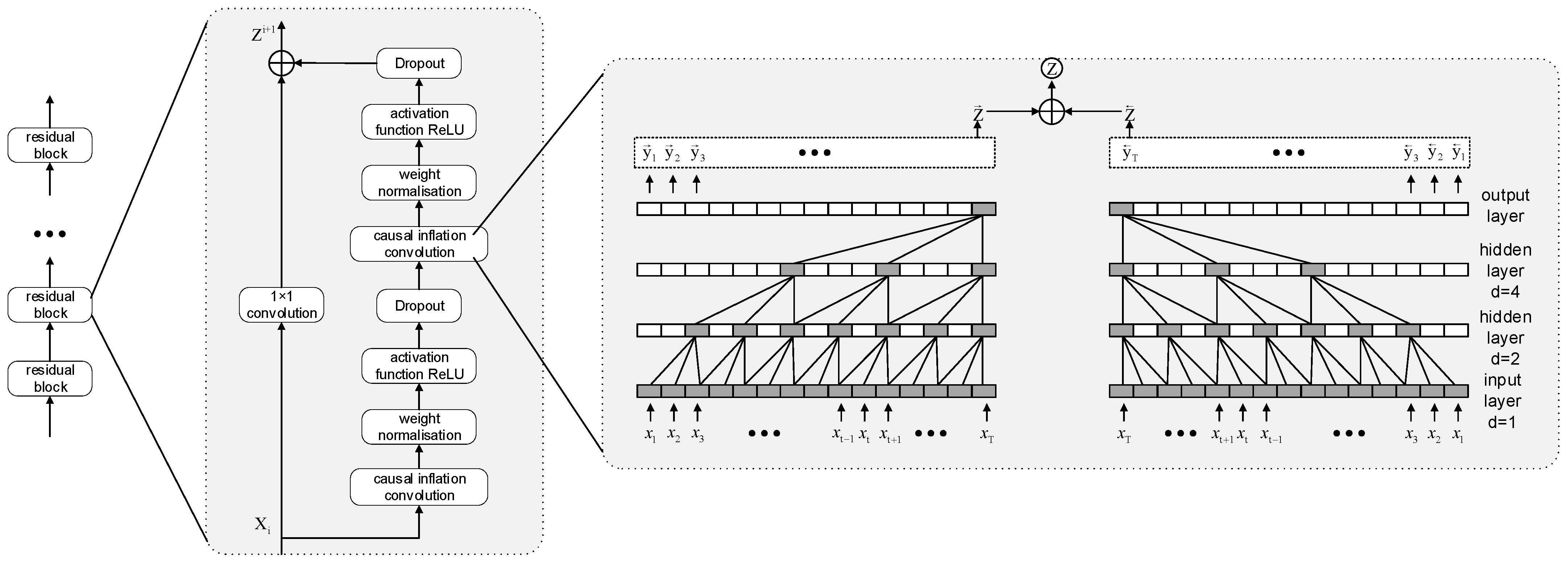
3.3. Bidirectional Time Convolution Network (BITCN)

The Temporal Convolutional Network (TCN) model utilizes the convolution operation derived from Convolutional Neural Networks (CNNs) and modifies it for time series data by incorporating causal and dilated convolutions. The causal convolution component is pivotal for ensuring the temporal integrity of predictions, as it constrains the convolution kernel’s movement direction to rely solely on current and past inputs, thereby preventing any influence from future data. The dilated convolution introduces intervals in the weight matrix of the convolution kernel through the application of an inflation factor, allowing the convolution operation to capture a broader receptive field without increasing the number of parameters. Furthermore, the incorporation of residual blocks in the TCN effectively addresses the challenges of gradient vanishing and explosion by adding residual pathways, thereby enhancing both the training efficiency and stability of the network. By incorporating a bidirectional information processing mechanism that learns features from both forward and reverse sequences, the model’s capacity to understand and predict time series data is significantly enhanced [30]. The structure of the BITCN is illustrated in Figure 3.

3.4. Bidirectional Gated Recirculation Unit (BIGRU)

The BiGRU is a specialized form of recurrent neural network (RNN) that integrates data inputs from both the forward and backward (Gated Recurrent Unit) GRU layers. This dual processing capability allows the model to analyze time series data from both directions simultaneously, thereby capturing more comprehensive and nuanced features. Compared to long short-term memory (LSTM) networks, the GRU is more streamlined in design, featuring only two gates: the reset gate and the update gate. Its architectural structure is illustrated in Figure 4. The reset gate value is produced by a sigmoid activation function, with outputs ranging from 0 to 1. A value closer to 0 indicates that the model is less likely to consider previous information, while a value closer to 1 signifies that the model retains more past information. Similarly, the update gate, also generated by a sigmoid activation function, functions in the same manner: values closer to 0 suggest that more new information is being introduced, whereas values closer to 1 indicate that the model retains more old information [31].

Based on the architecture of GRU neural network, the mathematical formulation of its forward propagation is as follows:

$$R_t=\sigma (X_t{W}_{\mathrm{xr}}+H_{t-1}{W}_{\mathrm{hr}}+b_{\mathrm{r}})$$

(13)

$$Z_t=\sigma (X_t{W}_{\mathrm{xz}}+H_{t-1}{W}_{\mathrm{hz}}+b_{\mathrm{z}})$$

(14)

$${\tilde{\mathit{H}}}_t=tanh[X_t{W}_{\mathrm{xh}}+(R_t\times H_{t-1})W_{\mathrm{hr}}+b_{\mathrm{h}}]$$

(15)

$$H_t=(1-Z_t)\times H_{t-1}+Z_t\times {\tilde{H}}_t$$

(16)

In the expression, $X_t$ represents the input, $H_{t-1}$ denotes the hidden state information from the previous time step, $W_{\mathrm{hr}}$ indicates the parameters to be learned (weights), $b_{\mathrm{r}}$ represents the bias, ${\tilde{H}}_t$ signifies the candidate hidden state, and the symbol $\times$ denotes the element-wise multiplication of vectors. $\sigma$ and $tanh$ are the activation functions.

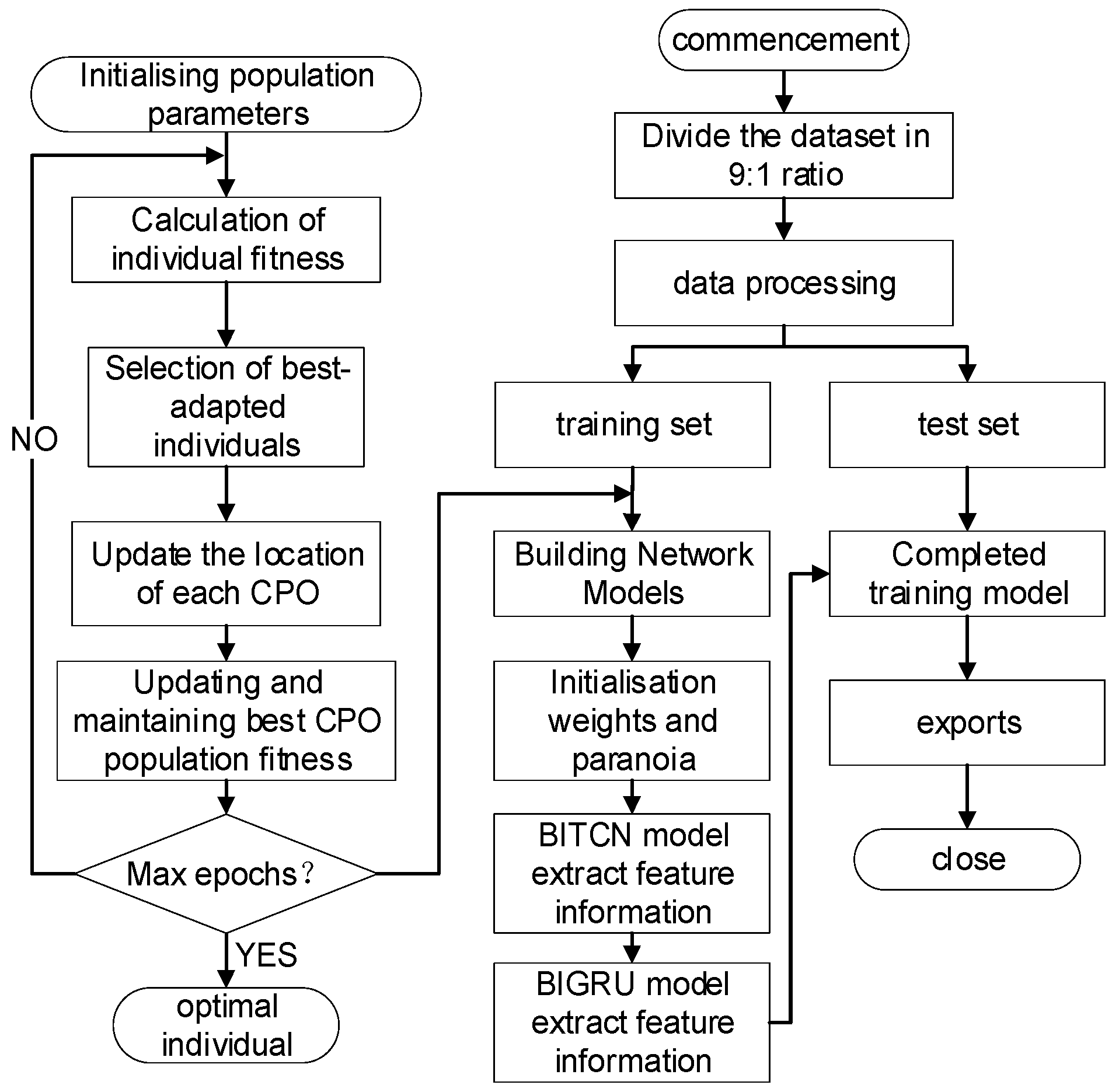
3.5. Convergent Modeling

The ICPO-BITCN-BIGRU model flowchart is shown in Figure 5.

The flow of the ICPO-BITCN-BIGRU model is illustrated below:

Step 1: Define the algorithmic parameters for the ICPO, including population size, maximum iterations, dimensionality, boundary constraints, and other intrinsic parameters of the ICPO algorithm.

Step 2: A random machine initializes the population, with each individual representing a specific set of hyperparameters, including the number of hidden layer nodes (Bi-GRU hidden units), the learning rate, the regularization parameter, and the number and size of convolutional kernels in the TCN.

Step 3: For each individual crown porcupine, construct the BITCN-BIGRU model, which includes an input layer, a TCN layer, a BiGRU layer with a designated number of hidden units, and a fully connected layer. Train the model on the training set and compute the mean square error (MSE) on the validation set to determine the fitness value.

Step 4: Sort the crown porcupine population based on the fitness function and select the best individual at that moment.

Step 5: Compare the current optimal solution with the previously stored optimal solution, and update the global optimal parameters if any improvements are identified.

Step 6: Determine whether the stopping condition has been met. If it has not, proceed to update the positions of the crown porcupine population to seek the next optimal solution. If the condition has been met, terminate the optimization process.

Step 7: The identified optimal parameters are incorporated into the BITCN-BIGRU model, which is then reconstructed to predict the pit monitoring points, resulting in the final output.

3.6. Data Pre-Processing

This research is mainly based on MATLAB 2022a and the hardware configuration is processor Intel^® Core™ i5-12400F (6 cores, 12 threads), graphics card NVIDIA GeForce RTX 3060 Ti (8 GB GDDR6) and RAM 32 GB DDR4 3200 MHz, with storage of 2 TB NVMe SSD (Samsung 980 Pro).

The dataset comprises a total of 410 periods of data collected from 27 October 2020 to 19 May 2021. Due to factors such as the Chinese New Year holiday, there are 14 periods with missing values at each detection point, resulting in a total of 378 periods of data with missing values. Consequently, this study employs the spline method to construct the curve. The steps of the cubic spline interpolation algorithm [32] are outlined below:

Step 1. Input data interpolation node $a=x_1<x_2<\dots <x_n=b$, corresponding function value $y_1,y_2,\cdots ,y_n$, boundary condition $y_1^{\prime }$ and $y_2^{\prime }$ and interpolation points to be found $x_0$.

Step 2. Calculate the length of each subinterval with the following formula:

$$h_j=x_{j+1}-x_j\hspace{1em}(j=1,2,\dots ,n-1)$$

(17)

Step 3. Calculate intermediate variables ${\mu }_j$ and $d_j$ with the following equations:

$${\mu }_j={\displaystyle \frac{h_{j-1}}{h_{j-1}+h_j}}$$

(18)

$$d_j=6\left({\displaystyle \frac{y_{j+1}-y_j}{h_j}}-{\displaystyle \frac{y_j-y_{j-1}}{h_{j-1}}}\right)\hspace{1em}(j=2,3,\dots ,n-1)$$

(19)

Step 4. Calculate intermediate variables ${\beta }_1$ and ${\beta }_n$ with the following equations:

$${\beta }_1=6\left({\displaystyle \frac{y_2-y_1}{h_1}}-y_1^{\prime }\right)$$

(20)

$${\beta }_n=6\left(y_n^{\prime }-{\displaystyle \frac{y_n-y_{n-1}}{h_{n-1}}}\right)$$

(21)

Step 5. Solve the final system of equations using the catch-up method.

Step 6. For each subinterval $[x_j,x_{j+1}]$, the expression for the output cubic spline interpolation function is shown below:

$$S_j(x)=a_j{(x-x_j)}^3+b_j{(x-x_j)}^2+c_j(x-x_j)+d_j$$

(22)

Step 7. Determine the sub-interval in which the interpolation point is located, and utilize the corresponding cubic spline function to compute the interpolation result.

The data obtained after interpolation using the cubic spline method are presented in

Table 2. Statistical table of cumulative changes at foundation pit monitoring points.

Number	DB48-1	DB48-2	……	ZQS50	……	ZQC46	ZQC50
1	0	0	……	0	……	0	0
2	−0.11	−0.14	……	0.04	……	0.12	0.01
3	−0.20	−0.34	……	0.06	……	0.25	0.04
4	−0.31	−0.84	……	0.08	……	0.24	0.08
5	−0.23	−1.14	……	0.09	……	0.23	0.12
6	−0.26	−1.42	……	0.10	……	0.23	0.16
……	……	……	……	……	……	……	……
206	−16.42	−16.84	……	6.092	……	3.16	2.08
207	−16.53	−16.53	……	6.08	……	3.17	2.13
208	−16.65	−16.85	……	6.08	……	3.16	2.15
209	−16.73	−17.23	……	6.083	……	3.15	2.16
……	……	……	……	……	……	……	……
406	−25.50	−25.45	……	5.39	……	3.96	2.00
407	−25.30	−25.61	………	5.38	………	3.97	2.01
408	−25.53	−25.59	……	5.37	……	3.98	2.02
409	−25.75	−25.67	……	5.34	……	3.99	2.03
410	−25.54	−25.82	……	5.27	……	4.00	2.05

below.

3.7. Indicators for Model Evaluation

There are several evaluation metrics for neural network prediction models, with the most common including the coefficient of determination (R²), root mean square error (RMSE), mean absolute error (MAE), and mean absolute percentage error (MAPE). R² is a statistic that measures model fit, taking values between [0, 1]; values close to 1 indicate a better fit of the model to the data, while values near 0 suggest a poor fit. RMSE quantifies the difference between predicted and actual values, with smaller RMSE values indicating better predictive performance of the model. MAE represents the average of the absolute differences between the true values and the predicted values; a smaller MAE indicates greater predictive accuracy. MAPE quantifies the average percentage error between the true and predicted values, facilitating the visualization of prediction errors relative to the true values. These four evaluation metrics provide a comprehensive assessment of the model’s predictive accuracy and reliability, as defined by the following formulas:

$$R^2=1-{\displaystyle \frac{{\displaystyle {\sum }_{i=1}^N{(y_i-{\widehat{y}}_i)}^2}}{{\displaystyle {\sum }_{i=1}^N{(y_i-\overline{y})}^2}}}$$

(23)

$$RMSE=\sqrt{{\displaystyle \frac{{\displaystyle {\sum }_{i=1}^N{(y_i-{\widehat{y}}_i)}^2}}{N}}}$$

(24)

$$MAE={\displaystyle \frac{{\displaystyle {\sum }_{i=1}^N\left|y_i-{\widehat{y}}_i\right|}}{N}}$$

(25)

$$MAPE={\displaystyle \frac{1}{N}}{\displaystyle {\sum }_{i=1}^N\left[\frac{\left|{\widehat{y}}_i-y_i\right|}{{\widehat{y}}_i}\right]}\times 100$$

(26)

In the formula, $N$ indicates the total number of forecast periods, $y_i$ denotes the monitored value, ${\widehat{y}}_i$ denotes the predicted value and $\overline{y}$ denotes the average of the monitored values.

3.8. Model Validation

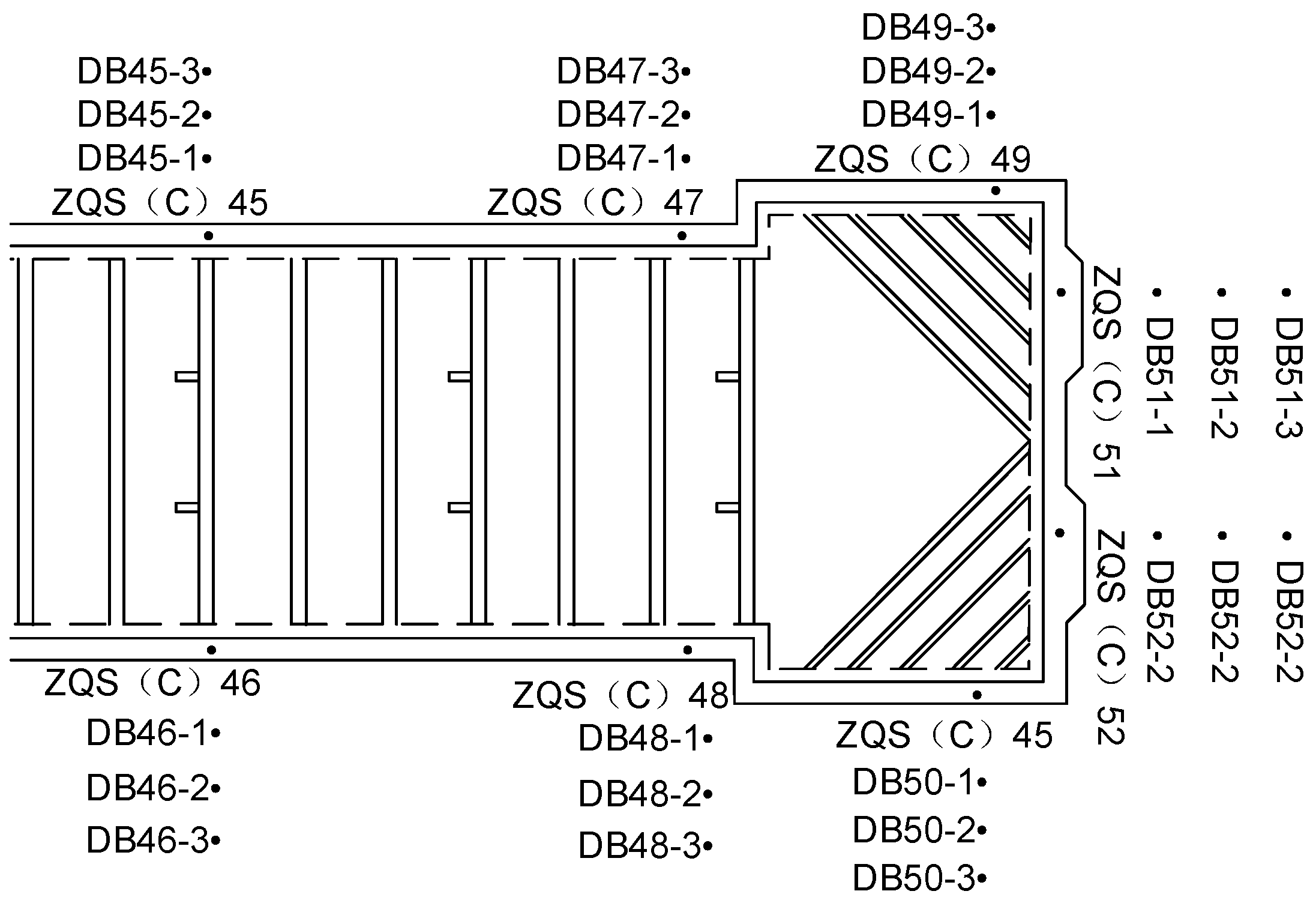
The optimal number of iterations, batch size, and number of neurons in the hidden layer identified by the ICPO algorithm were employed in training the BITCN-BIGRU model. Upon completion of the training, the test set data were input into the model to generate prediction results. These results were subsequently compared and analyzed against those from other prediction models. The dataset comprised a total of 410 entries, spanning from 27 October 2020 to 19 May 2021 and included underground pit monitoring data from 27 monitoring points, which served as multi-feature indicators for predicting the DB48-2 monitoring point. The prediction accuracy of the ICPO-BITCN-BIGRU model, along with other models, is presented in

Table 3. Table of prediction accuracy of each model.

NAME	MAE	MAPE	RMSE	R2
ICPO-BITCN-BIGRU	0.0449	0.1745	0.0522	0.9936
CPO-BITCN-BIGRU	0.1248	0.4886	0.1317	0.9589
DBO-BITCN-BIGRU	0.1201	0.4712	0.1325	0.9585
CNN-Attention-LSTM	0.1908	0.6063	0.1568	0.9138
BITCN-BIGRU	0.1711	0.6647	0.1937	0.9111
CNN-LSTM	0.2078	0.8041	0.2435	0.8597

.

The ICPO-BITCN-BIGRU model achieved values of MAE, MAPE, RMSE, and R² of 0.0449, 0.1745, 0.0522, and 0.9936, respectively. In comparison, the CPO-BITCN-BIGRU, DBO-BITCN-BIGRU, and CNN-Attention-LSTM models exhibited reductions in MAE by 78%, 76%, and 71%; in MAPE by 62.6%, 63%, and 60.6%; and in RMSE by 76.5%, 71.2%, and 66.7%, respectively. Additionally, the coefficient of determination R² for the ICPO-BITCN-BIGRU model is the closest to 1, indicating a superior fitting ability to the measured values compared to the other prediction models. Overall, the ICPO-BITCN-BIGRU model demonstrated better prediction accuracy and fitting performance compared to the multi-feature CNN-LSTM and BITCN-BIGRU prediction models.

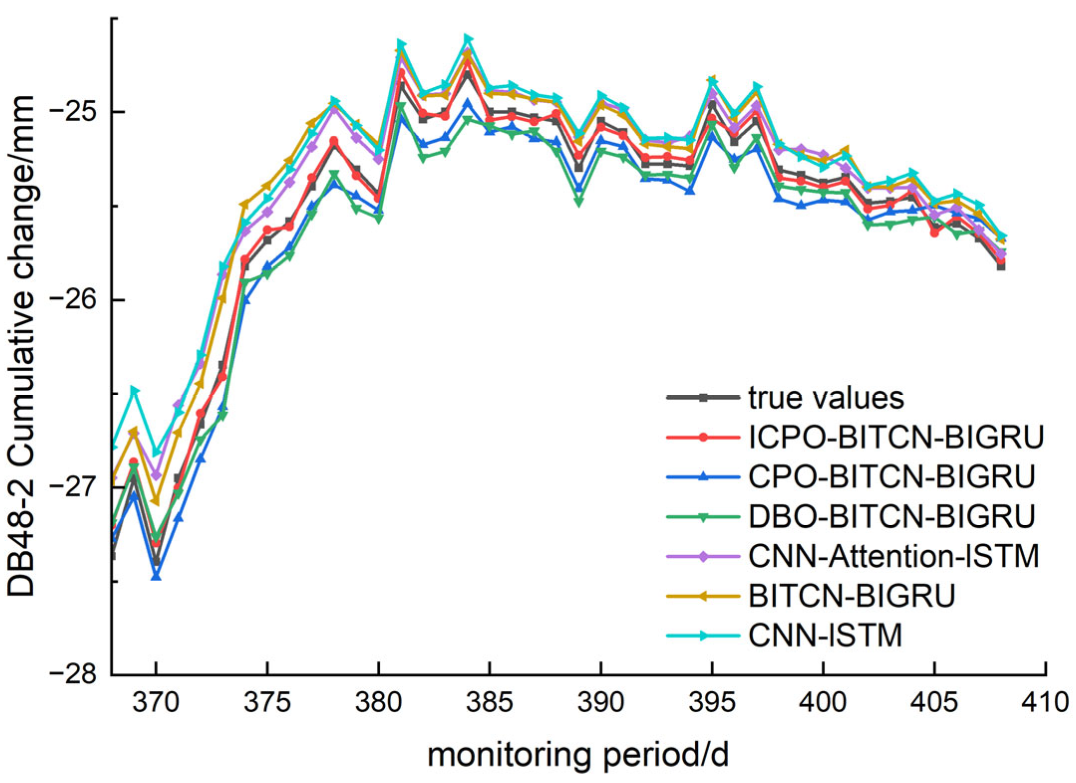
The comparison of predicted and true values for the ICPO-BITCN-BIGRU model alongside other prediction models is illustrated in Figure 6. The figure indicates that the predicted deformation trends for the ICPO-BITCN-BIGRU, CPO-BITCN-BIGRU, and DBO-BITCN-BIGRU models closely align with the true deformation trends, demonstrating a strong fit. In contrast, the predicted values from the BITCN-BIGRU, CNN-Attention-LSTM, and CNN-LSTM models exhibit significant discrepancies from the true values in certain data points. This deformation prediction analysis confirms that the ICPO algorithm outperforms the traditional CPO and DBO algorithms in optimizing the BITCN-BIGRU model. Furthermore, the ICPO-BITCN-BIGRU model demonstrates superior prediction performance compared to the CNN-Attention-LSTM model, making it more suitable for this project.

4. Deformation Prediction of the ICPO-BITCN-BIGRU Model

The previous section’s prediction of pit deformation focused solely on the surface settlement monitoring point, without accounting for other deformation aspects within the project. To enhance the evaluation of pit deformation prediction, it is essential to compare the effectiveness of predictions across additional monitoring points. Therefore, surface settlement, horizontal displacement at the pile top, and vertical displacement at the pile top have been selected as key characteristic points for prediction.

In this chapter, a multi-feature BITCN-BIGRU combinatorial neural network model is constructed using the detection data from monitoring point DB48-2 and its 27 nearby monitoring points as feature indicators. This model is designed to extract spatial and temporal features from the pit data. The performance of the ICPO-BITCN-BIGRU model is then compared with that of several other models, including CPO-BITCN-BIGRU, Convolutional Neural Network (CNN), Long Short-Term Memory (LSTM), Gated Recurrent Unit (GRU), and Historical Average (HA).

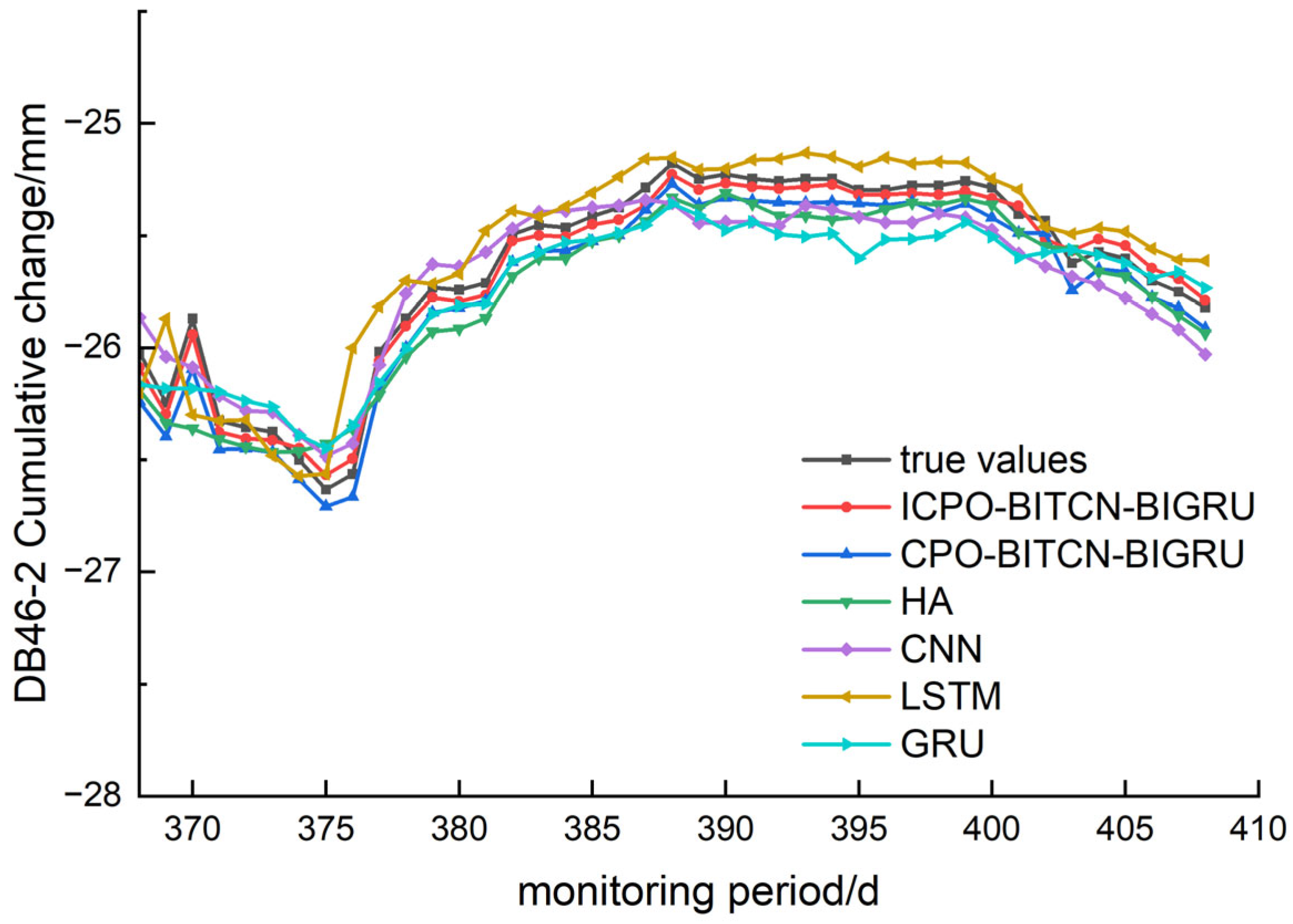
4.1. Prediction of Surface Settlement Deformation

The prediction of the three surface settlement monitoring points—DB48-2, DB46-2, and DB50-2—was evaluated by comparing the index values and prediction effects of various models. This comparison was conducted using evaluation metrics such as R², MAE, RMSE, and MAPE, as illustrated in Figure 7, Figure 8, and Figure 9, respectively. The detailed results of this analysis are summarized in

Table 4. Table of prediction accuracy of prediction model for each monitoring point.

Monitoring Point	Predictive Modeling	MAE	MAPE	RMSE	R2
DB48-2	HA	0.3646	1.4275	0.3985	0.6241
	CNN	0.2867	1.1200	0.3331	0.7373
	LSTM	0.1576	0.6090	0.2075	0.8981
	GRU	0.2671	1.0461	0.2920	0.7982
	CPO-BITCN-BIGRU	0.1248	0.4886	0.1317	0.9589
	ICPO-BITCN-BIGRU	0.0449	0.1745	0.0522	0.9936
DB46-2	HA	0.1326	0.5165	0.1508	0.8722
	CNN	0.1331	0.5193	0.1441	0.8832
	LSTM	0.1262	0.4897	0.1665	0.8441
	GRU	0.1506	0.5888	0.1682	0.8410
	CPO-BITCN-BIGRU	0.1055	0.4109	0.1114	0.9303
	ICPO-BITCN-BIGRU	0.0475	0.1851	0.0496	0.9862
DB50-2	HA	0.2039	0.7888	0.2180	0.7714
	CNN	0.2176	0.8402	0.2390	0.7254
	LSTM	0.1619	0.6257	0.1919	0.8229
	GRU	0.1525	0.5907	0.1688	0.8630
	CPO-BITCN-BIGRU	0.1460	0.5641	0.1547	0.8849
	ICPO-BITCN-BIGRU	0.0940	0.3635	0.0980	0.9538

.

A comprehensive analysis of the aforementioned images and graphs demonstrates that the ICPO-BITCN-BIGRU prediction model proposed in this study outperforms other models across various error indicators when predicting changes in surface settlement. The model exhibits stable prediction accuracy, strong generalization capability, and a high degree of goodness of fit. The prediction results indicate that the ICPO-BITCN-BIGRU model effectively captures the deformation patterns and trends over time in the numerical data derived from pit engineering monitoring.

For the MAE, the prediction error values at the selected monitoring sites for the ICPO-BITCN-BIGRU model were 0.0449, 0.0475, and 0.0940. In comparison, the CPO-BITCN-BIGRU model exhibited error values of 0.1248, 0.1198, and 0.1460, while the LSTM model recorded error values of 0.1576, 0.1262, and 0.1619. The CNN model showed error values of 0.2867, 0.1331, and 0.2176, respectively. The results indicate that for the three selected measurement points, the order of prediction accuracy is as follows: ICPO-BITCN-BIGRU < CPO-BITCN-BIGRU < other models, demonstrating that the ICPO-BITCN-BIGRU model provides the most accurate predictions.

For the MAPE, the prediction error values at the selected monitoring points for the ICPO-BITCN-BIGRU model were 0.1745, 0.1851, and 0.3635. In comparison, the CPO-BITCN-BIGRU model exhibited error values of 0.4886, 0.4109, and 0.5641. The LSTM model recorded error values of 0.6090, 0.4897, and 0.6257, while the CNN model showed error values of 1.1200, 0.5193, and 0.8402, respectively. These results indicate that for the three selected measurement points, the order of prediction accuracy is as follows: ICPO-BITCN-BIGRU < CPO-BITCN-BIGRU < other models. This demonstrates that the ICPO-BITCN-BIGRU model provides more accurate predictions compared to the other models evaluated.

For the coefficient of determination R², the prediction error values at the selected monitoring points for the ICPO-BITCN-BIGRU model were 0.9936, 0.9862, and 0.9538. In comparison, the CPO-BITCN-BIGRU model exhibited R² values of 0.9589, 0.9303, and 0.8849. The LSTM model recorded R² values of 0.8981, 0.8441, and 0.8229, while the CNN model showed R² values of 0.7373, 0.8832, and 0.7254, respectively.

These results indicate that for the three selected measurement points, the coefficients of determination for the HA, CNN, LSTM, and GRU prediction models are all smaller than those of the ICPO-BITCN-BIGRU model. The R² values for the ICPO-BITCN-BIGRU model are closer to 1, suggesting that its linear relationship between predicted and actual values is optimal among the compared models. Consequently, the prediction results from the ICPO-BITCN-BIGRU model are closer to the real values, indicating its superior performance in this context.

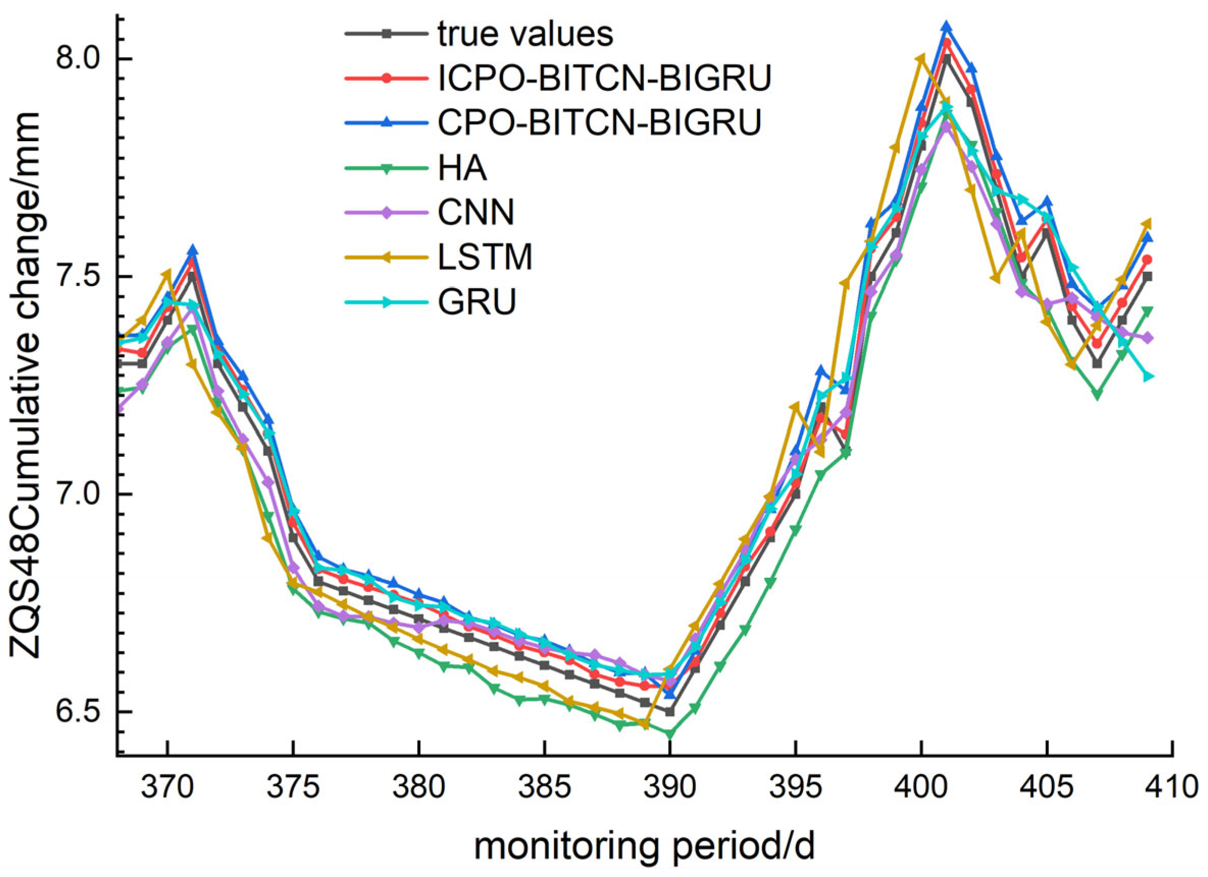
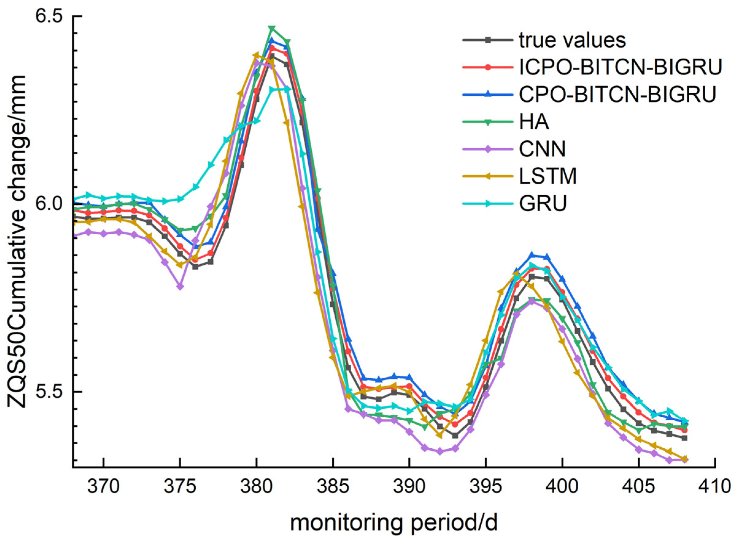
4.2. Prediction of Horizontal Displacement and Deformation at the Top of Pile

To predict horizontal displacement and deformation at the top of the pile, three monitoring points—ZQS46, ZQS48, and ZQS50—were selected. Comparative graphs illustrating the evaluation metrics and prediction performance of various models are presented in Figure 10, Figure 11 and Figure 12. The analysis encompasses MAE, RMSE, MAPE and R², as summarized in

Table 5. Table of prediction accuracy of prediction model for each monitoring point.

Monitoring Point	Predictive Modeling	MAE	MAPE	RMSE	R2
ZQS46	HA	0.0233	0.7203	0.0243	0.8865
	CNN	0.0239	0.7347	0.0267	0.8631
	LSTM	0.0174	0.5296	0.0283	0.8471
	GRU	0.0184	0.5694	0.0211	0.9148
	CPO-BITCN-BIGRU	0.0141	0.4357	0.0145	0.9597
	ICPO-BITCN-BIGRU	0.0070	0.2151	0.0076	0.9888
ZQS48	HA	0.0830	1.1717	0.0890	0.9564
	CNN	0.0673	0.9407	0.0756	0.9685
	LSTM	0.1065	1.4784	0.1275	0.9104
	GRU	0.0634	0.8890	0.0773	0.9670
	CPO-BITCN-BIGRU	0.0699	0.9801	0.0736	0.9701
	ICPO-BITCN-BIGRU	0.0334	0.4713	0.0348	0.9933
ZQS50	HA	0.0533	0.9183	0.0580	0.9778
	CNN	0.0777	1.3354	0.0872	0.9499
	LSTM	0.0719	1.2288	0.0931	0.9428
	GRU	0.0751	1.2757	0.0945	0.9411
	CPO-BITCN-BIGRU	0.0541	0.9368	0.0558	0.9795
	ICPO-BITCN-BIGRU	0.0249	0.4313	0.0259	0.9956

.

For the selected monitoring points, the ICPO-BITCN-BIGRU model, CPO-BITCN-BIGRU model, LSTM model, CNN model, and GRU model were employed to predict trends in the monitoring data. Notably, the HA and CNN models exhibited significant discrepancies in their predicted values at both troughs and peaks. In contrast, the ICPO-BITCN-BIGRU and CPO-BITCN-BIGRU models demonstrated robust generalization capabilities, effectively handling monitoring data characterized by substantial fluctuations. Additionally, the GRU model showed considerable divergence between its predicted trends and the actual values at each monitoring point.

For the MAE, the prediction error values at the selected monitoring sites for the ICPO-BITCN-BIGRU model were 0.0070, 0.0334, and 0.0249. In comparison, the CPO-BITCN-BIGRU model exhibited error values of 0.0141, 0.0699, and 0.0541. The LSTM model recorded error values of 0.0174, 0.1065, and 0.0719, while the CNN model reported error values of 0.0239, 0.0673, and 0.0777. These results indicate the following order of performance: ICPO-BITCN-BIGRU < CPO-BITCN-BIGRU < other models, demonstrating that the ICPO-BITCN-BIGRU model achieved the best prediction results.

For the MAPE, the prediction error values at the selected monitoring sites for the ICPO-BITCN-BIGRU model were 0.2151, 0.4713, and 0.4313. In comparison, the CPO-BITCN-BIGRU model exhibited error values of 0.4357, 0.9801, and 0.9368. The LSTM model recorded error values of 0.5296, 1.4784, and 1.2288, while the CNN model showed error values of 0.7347, 0.9407, and 1.3354, respectively. These results indicate that the ICPO-BITCN-BIGRU model outperformed the other models in terms of prediction accuracy at the selected monitoring sites.

For the RMSE, the ICPO-BITCN-BIGRU model demonstrated prediction error values of 0.0076, 0.0348, and 0.0259 at the selected monitoring sites. In comparison, the CPO-BITCN-BIGRU model exhibited RMSE values of 0.0145, 0.0736, and 0.0558. The LSTM model recorded RMSE values of 0.0283, 0.1275, and 0.0931, while the CNN model reported RMSE values of 0.0267, 0.0756, and 0.0872, respectively. These results indicate that the RMSE for the three selected measurement points follows the order: ICPO-BITCN-BIGRU < CPO-BITCN-BIGRU < other models, underscoring the superior predictive performance of the ICPO-BITCN-BIGRU model.

For the coefficient of determination R², the ICPO-BITCN-BIGRU model demonstrated values of 0.9888, 0.9933, and 0.9956 at the selected monitoring points. In contrast, the CPO-BITCN-BIGRU model achieved R² values of 0.9597, 0.9701, and 0.9795. The LSTM model recorded values of 0.8471, 0.9104, and 0.9428, while the CNN model yielded values of 0.8631, 0.9685, and 0.9499. These findings indicate that for the three selected measurement points, the coefficients of determination for the HA, CNN, LSTM, and GRU models are consistently lower than those for the ICPO-BITCN-BIGRU model. The R² values of the ICPO-BITCN-BIGRU model are notably closer to 1, reflecting an optimal linear relationship between predicted and actual values, and indicating that its predictions are more closely aligned with the observed data.

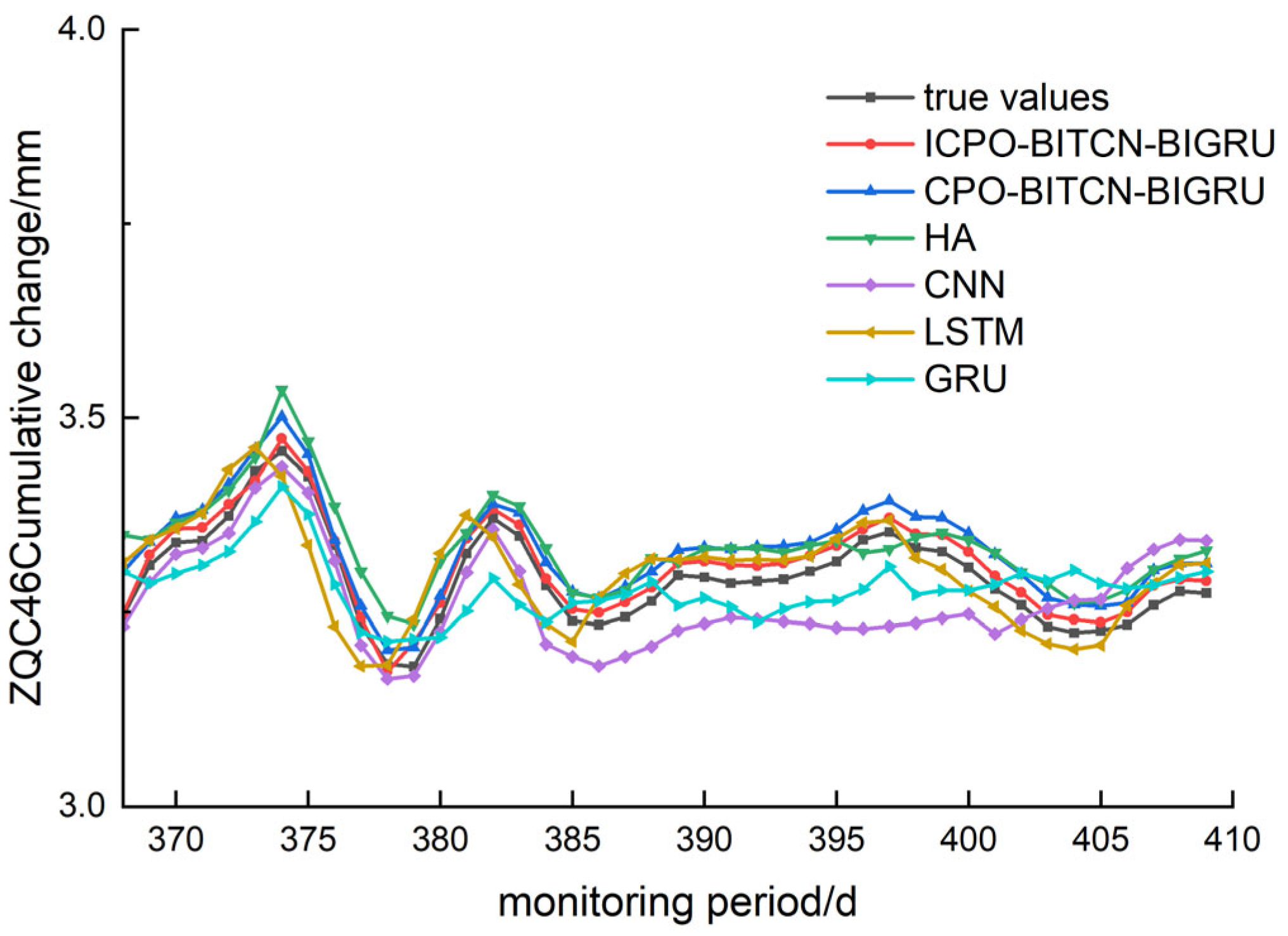
4.3. Prediction of Vertical Displacement and Deformation at the Top of Pile

To predict the vertical displacement of pile tops, three monitoring points—ZQC50, ZQC48, and ZQC46—were selected. The comparison graphs illustrating the evaluation index values and prediction performance of various models are presented in Figure 13, Figure 14 and Figure 15. Comparative analyses were conducted using metrics such as R², MAE, RMSE, and MAPE, as detailed in

Table 6. Table of prediction accuracy of prediction model for each monitoring point.

Monitoring Point	Predictive Modeling	MAE	MAPE	RMSE	R2
ZQC50	HA	0.0601	1.5702	0.0688	0.6973
	CNN	0.0852	2.2236	0.0972	0.3957
	LSTM	0.0506	1.3285	0.0541	0.8131
	GRU	0.0704	1.8420	0.0750	0.6409
	CPO-BITCN-BIGRU	0.0461	1.2114	0.0476	0.8555
	ICPO-BITCN-BIGRU	0.0187	0.4914	0.0191	0.9768
ZQC46	HA	0.0414	1.2599	0.0450	0.4675
	CNN	0.0471	1.4291	0.0550	0.2019
	LSTM	0.0369	1.1176	0.0426	0.5212
	GRU	0.0426	1.2893	0.0465	0.4304
	CPO-BITCN-BIGRU	0.0350	1.0636	0.0362	0.6551
	ICPO-BITCN-BIGRU	0.0162	0.4917	0.0170	0.9238
ZQC48	HA	0.0093	0.4920	0.0100	0.9709
	CNN	0.0223	1.1623	0.0236	0.8388
	LSTM	0.0109	0.5765	0.0117	0.9606
	GRU	0.0118	0.6247	0.0122	0.9571
	CPO-BITCN-BIGRU	0.0092	0.4838	0.0094	0.9746
	ICPO-BITCN-BIGRU	0.0042	0.2245	0.0045	0.9943

.

For the MAE, the ICPO-BITCN-BIGRU model achieved prediction error values of 0.0187, 0.0162, and 0.0042 for the selected monitoring sites. In comparison, the CPO-BITCN-BIGRU model recorded MAE values of 0.0461, 0.0350, and 0.0092. The LSTM model had an MAE of 0.0506, while the CNN model reported error values of 0.0852, 0.0471, and 0.0223, respectively. This indicates the following order of performance: ICPO-BITCN-BIGRU < CPO-BITCN-BIGRU < other models, with the ICPO-BITCN-BIGRU model demonstrating the best prediction results.

For the MAPE, the ICPO-BITCN-BIGRU model exhibited prediction error values of 0.4914, 0.4917, and 0.2245 at the selected monitoring sites. In contrast, the CPO-BITCN-BIGRU model recorded MAPE values of 1.2114, 1.0636, and 0.4838. The LSTM model yielded error values of 1.3285, 1.1176, and 0.5765, while the CNN model demonstrated MAPE values of 2.2236, 1.4291, and 1.1623, respectively.

For the RMSE, the ICPO-BITCN-BIGRU model demonstrated prediction error values of 0.0191, 0.0170, and 0.0045 at the selected monitoring sites. In comparison, the CPO-BITCN-BIGRU model recorded RMSE values of 0.0476, 0.0362, and 0.0094. The LSTM model exhibited RMSE values of 0.0541, 0.0426, and 0.0117, while the CNN model showed error values of 0.3957, 0.2019, and 0.0236. These results indicate that the RMSE for the three selected monitoring points follows the order: ICPO-BITCN-BIGRU < CPO-BITCN-BIGRU < other models.

For the coefficient of determination R², the ICPO-BITCN-BIGRU model yielded values of 0.9768, 0.9238, and 0.9943 at the selected monitoring points. In contrast, the CPO-BITCN-BIGRU model recorded R² values of 0.8555, 0.6551, and 0.9746, while the LSTM model exhibited values of 0.8131, 0.5212, and 0.9606. The CNN model demonstrated R² values of 0.3957, 0.2019, and 0.8388. These results indicate that the coefficients of determination for the HA, CNN, LSTM, and GRU prediction models are consistently lower than those of the ICPO-BITCN-BIGRU model. Notably, the R² values for the ICPO-BITCN-BIGRU model are closer to 1, indicating an optimal linear relationship between the predicted and actual values, and suggesting that its prediction results are more closely aligned with the true values compared to the other models.

5. Conclusions

Based on a metro pit construction project in Chengdu, this paper provides an overview of the project, addresses the interpolation and filling of missing data using the pit monitoring data, and further predicts pit deformation employing the ICPO-BITCN-BIGRU model. The study ultimately arrives at the following conclusions:

(1) The cumulative change in the surface at DB48-2, a pit monitoring point, was selected as the research subject. Various prediction models, including ICPO-BITCN-BIGRU, CPO-BITCN-BIGRU, DBO-BITCN-BIGRU, CNN-Attention-LSTM, BITCN-BIGRU, and CNN-LSTM, were validated through experiments. The results indicate that the ICPO-BITCN-BIGRU model demonstrated the best fitting prediction performance among the samples, with the MAE of the predictions decreasing from 0.2867 to 0.0449. This model is specifically tailored for predicting deep foundation pit deformation, significantly enhancing both the accuracy and reliability of the predictions.

(2) The CPO-BITCN-BIGRU, CNN, LSTM, GRU, and HA prediction models were constructed and compared with the ICPO-BITCN-BIGRU model presented in this study to predict the changes in the cumulative values at nine monitoring points, including DB48-2, DB46-2, and DB50-2, which are associated with the foundation pit. Overall, the prediction models exhibited a general consistency with the actual values in forecasting the trends of pit deformation. However, all models displayed some degree of error, particularly at the peaks and valleys of the deformation curve, where discrepancies were more pronounced.

(3) Taking the RMSE evaluation index of the pile top vertical displacement monitoring points as an example, the CNN model recorded errors of 0.3957, 0.2019, and 0.0236, while the LSTM model exhibited errors of 0.8131, 0.5212, and 0.9606. The CPO-BITCN-BIGRU model showed errors of 0.0476, 0.0362, and 0.0094, and the ICPO-BITCN-BIGRU model achieved errors of 0.0191, 0.0170, and 0.0045, respectively. The comparison of test results indicates that the ICPO-BITCN-BIGRU prediction model demonstrates superior performance. Notably, the predicted values from the ICPO-BITCN-BIGRU model align closely with the actual values, yielding R² values of 0.9768, 0.9238, and 0.9943, respectively, indicating a strong agreement with the real data. Therefore, the ICPO-BITCN-BIGRU model constructed in this study exhibits high prediction accuracy and stability, making it suitable for application in practical engineering scenarios.