Comparative Analysis of Machine Learning Models for Predicting Contaminant Concentration Distributions in Hospital Wards

Abstract

As the distribution of indoor contaminants is often heterogeneous, the traditional Wells–Riley equation is inadequate for accurately assessing the infection risk to indoor personnel. In this study, contaminant concentration data from hospital wards were obtained through experimentally validated computational fluid dynamics (CFD) simulations. Four common machine learning models—multiple linear regression (MLR), support vector regression (SVR), backpropagation (BP) neural network, and convolutional neural network (CNN)—were employed to predict the distribution of contaminants within the wards. The results demonstrate that the CNN achieves the best predictive performance, followed by the BP neural network. Specifically, the CNN exhibited a root mean square error, mean absolute error, and mean absolute percentage error of 6.31 ppm, 3.18 ppm, and 8.33%, respectively. Comparative analysis revealed that the CNN reduced the mean absolute percentage error (MAPE) by 58.18%, 33.47%, and 25.15% compared to MLR, SVR, and BPNN, respectively.

1. Introduction

Worldwide, losses from respiratory infectious disease pandemics, notably, SARS and COVID-19, have been enormous, and research into how to effectively anticipate and quantify the risk of infection with such infections has received increasing attention. The Wells–Riley equation is a model for calculating the probability of infection, obtained by Riley et al. in 1978 to calculate the probability of infection on the basis of an analysis of a measles epidemic in an elementary school with 836 students [1]. Hospital wards are a critical component of the health care environment, but they also represent a high-risk area for pathogen transmission. According to statistics, approximately 1.4 million health care-associated infections (HAIs) occur worldwide each year, resulting in the exacerbation of existing conditions and even death for many patients [2]. Furthermore, HAIs significantly increase health care costs, with estimates suggesting that 7 out of every 100 hospitalized patients in developed countries will be affected by at least one HAI; in developing countries, this proportion can reach as high as 10% [3]. Air quality and airflow patterns within hospital wards have direct impacts on infection transmission.

It is one of the most common models for calculating the probability of infection among indoor workers and has been applied to predict infection probabilities in different scenarios, such as office buildings, buses, and hospitals [4,5,6]. Moreover, scholars have continuously modified the Wells–Riley equation to improve the accuracy of its predictions [7,8]. The Wells–Riley equation assumes that contamination is uniformly distributed throughout space, but in practice, the spatial distribution of contamination is often not uniform [9,10]. Lu et al. studied the proportion of indoor contamination under four airflow structures—an interstory air supply, mixed ventilation, downdraft ventilation, and displacement ventilation—and they reported that contamination was unevenly distributed under different airflow patterns [11]. Cho studied the distributions of contamination under three ventilation strategies and reported that the diffusion patterns of contamination were different under the different ventilation strategies [12], which also proves that pollution is not always distributed uniformly in space. Therefore, the traditional Wells–Riley equation cannot be used to assess the infection risk of indoor personnel accurately.

Currently, the expanded Wells–Riley equation developed by Zhang et al. is used by the majority of researchers to assess the risk of infection in individuals exposed to a variety of spatial contaminants [8]. Liu et al. used CFD to determine the contaminant distribution in a multicompartment dental clinic and combined it with the extended Wells–Riley method to analyze the risks of infection in different areas within the clinic [6]. Luo et al. used CFD to simulate the distribution of contaminants in a coach and combined it with the extended Wells–Riley method to analyze the infection risk of people on the coach [13]. Zhang et al. used CFD to simulate the concentration field in a hospital ward and combined it with an extended Wells–Riley model to analyze the risks of infection in the ward under different airflow patterns [14]. On the basis of the above study, CFD is required to obtain the indoor contamination distribution to accurately predict the infection probabilities of people in the room. However, CFD modeling and solving take a long time, and it is difficult to quickly obtain indoor contamination distributions via CFD. Therefore, quickly predicting indoor contamination distributions is currently an important challenge. The rapid prediction of indoor contamination distributions can reveal real-time infection risks for health care workers and provide a basis for developing accurate outbreak prevention and control measures.

Convolutional neural networks are also widely used in medical image analysis, environment sensing in self-driving vehicles, and other fields, where these application scenarios require accurate parsing of complex spatial information. Wei et al. [15] applied a deep dense SR (DDSR) convolutional neural network model to improve the resolution of medical images. Mishra et al. [16] presented an automatic traffic sign recognition system to minimize motor vehicle accidents using representation to identify signs; this task uses a deep convolutional neural network. In environments such as hospital wards, the distribution of contaminants is influenced not only by airflow but also by the room structure, equipment layout, etc. CNNs are good at automatically extracting complex spatial features from both 2D and 3D data, making them particularly effective at capturing patterns in indoor contaminant distributions [17].

Portal-Porras et al. performed CFD simulations on 158 different DU91W(2)250 airfoils, and the results indicated that CNNs are able to accurately predict the main characteristics of the flow around the flow control device [18]. Bhatnagar et al. used a CNN for flow field prediction and reported that velocity and pressure fields can be estimated efficiently and faster than can RANS solvers using CNN modeling, which allows for near real-time study of the effects of airfoil shape and operating conditions on aerodynamic and flow fields [19]. In addition, multiple linear regression (MLR) and backpropagation (BP) neural networks are also commonly used in flow field prediction models. Tian et al. used MLR and BP neural networks to predict relative humidity, air age, and air exchange efficiency metrics, and their results revealed that the RMSE values for relative humidity, air age, and air exchange efficiency were 0.1, 29 s, and 0.1, respectively, when BP neural networks were used [20]. Liu et al. used BP neural networks to predict indoor temperatures, and their results revealed that the error induced when predicting indoor temperatures using a BP neural network was only 0.02 K [21]. Warey et al. used MLR and BP neural networks to predict the equivalent temperature in a compartment, and the results revealed that the average absolute percentage error was less than 5% [22]. The abovementioned studies demonstrate that machine learning achieves good results when applied to the rapid prediction of indoor flow fields, but few scholars have considered its application to the rapid prediction of indoor contamination distributions, especially in ward environments, which has not been fully explored.

In this study, as shown in Figure 1, we systematically applied multiple machine learning models to rapidly predict contaminant distributions in hospital wards, utilizing experimentally validated CFD data for rigorous training and testing. Notably, we found that convolutional neural networks (CNNs) significantly outperform other models in terms of prediction accuracy, which is crucial for enabling real-time monitoring of contaminant distributions in hospital environments. Furthermore, through a comprehensive comparison of various models, such as MLR, SVR, and BP neural networks, this study not only reveals the characteristics and applicable scenarios of each model but also provides a valuable reference for future research.

2. Method

2.1. Correlation Analysis

Sensors can accurately determine the contamination concentration at the current location, but a single sensor cannot accurately assess the indoor contamination distribution because of the uneven distribution of indoor contamination. Considering the cost of sensors, it is also impractical to arrange many sensors in a room. Therefore, an accurate indoor contamination distribution prediction method based on the arrangement of limited sensors is needed. Indoor contamination is influenced by indoor airflow and often diffuses from one area to adjacent areas, and there is a potential relationship between the contamination concentrations in different areas, so the contamination concentrations in representative areas of the room should be monitored. Correlation analysis involves analyzing two or more variable elements that have a correlation so that the closeness of the correlation between the two variable factors can be measured. Therefore, correlation analysis can be used to analyze the correlations of contamination concentrations in various indoor areas and identify representative indoor areas. In this study, Pearson’s correlation, the most common type of correlation analysis, was used [23]. The Pearson correlation coefficient is defined as the ratio of the covariance and standard deviation between two variables, and its equation can be expressed as

$$\mathrm{r}={\displaystyle \frac{{\sum }_{\mathrm{i}=1}^{\mathrm{n}}({\mathrm{X}}_{\mathrm{i}}-\overline{\mathrm{X}})({\mathrm{Y}}_{\mathrm{i}}-\overline{\mathrm{Y}}))}{\sqrt{{\sum }_{\mathrm{i}=1}^{\mathrm{n}}{({\mathrm{X}}_{\mathrm{i}}-\overline{\mathrm{X}})}^2}\sqrt{{\sum }_{\mathrm{i}=1}^{\mathrm{n}}{({\mathrm{Y}}_{\mathrm{i}}-\overline{\mathrm{Y}})}^2}}}$$

(1)

where $\overline{\mathrm{X}}$ is the average contamination concentration in one region of the variable; $\overline{\mathrm{Y}}$ is the average contamination concentration in another region; ${\mathrm{X}}_{\mathrm{i}}$ is the contamination concentration in one region in case i; and ${\mathrm{Y}}_{\mathrm{i}}$ is the contamination concentration in another region in case i.

2.2. Machine Learning

Machine learning is the process of making model assumptions about a given research problem, using computers to learn from the training data to obtain model parameters and ultimately to predict and analyze the data. Typical machine learning models include classification, regression, clustering, anomaly detection, dimensionality reduction, and reward maximization models [24]. Contamination concentration prediction is a regression problem. In this study, multiple linear regression, support vector machine regression, a backpropagation neural network, and a convolutional neural network are used to predict indoor contamination concentrations. These common models for machine learning are described below.

2.2.1. Multiple Linear Regression

Multiple linear regression (MLR) considers the effects of multiple factors on the same result. Equation (2) shows the MLR formula.

$${\mathrm{y}}_{\mathrm{i}}\left({\mathrm{x}}_{\mathrm{i}}\right)={\sum }_{\mathrm{j}=1}^{\mathrm{n}}{\mathsf{\omega }}_{\mathrm{j}}{\mathrm{x}}_{\mathrm{i}\mathrm{j}}+\mathrm{b}$$

(2)

where y is the predicted contamination concentration value; $\mathsf{\omega }$ denotes the weight coefficients; x represents the input variables; j is the serial number of the input parameter; and $\mathrm{b}$ is a constant term.

2.2.2. Support Vector Regression

Support vector regression (SVR) is an extension of an SVM, which is a statistics-based machine learning method proposed by Drucker et al. in 1996 [25]. The basic idea is to nonlinearly transform the input sample space to another high-dimensional space and construct a regression estimation function in this high-dimensional space; the regression equation can be expressed as

$${\mathrm{y}}_{\mathrm{i}}\left({\mathrm{x}}_{\mathrm{i}}\right)={\sum }_{\mathrm{j}=1}^{\mathrm{n}}{\mathsf{\omega }}_{\mathrm{j}}\phi {(\mathrm{x}}_{\mathrm{i}\mathrm{j}})+\mathrm{b}$$

(3)

where y is the predicted contamination concentration value; $\mathsf{\omega }$ denotes the weight coefficients; x represents the input variables; j is the serial number of the input parameter; $\mathrm{b}$ is a constant term; and $\phi$ is the mapping function, which serves to map the input samples to a higher-dimensional space.

The SVR is different from traditional regression models. Traditional regression models usually calculate losses directly on the basis of the difference between the predicted contamination concentration f(x) and the actual contamination concentration y. In contrast, SVR assumes that the deviation between f(x) and y that can be tolerated is ε. Therefore, the loss is calculated only when the absolute value of the deviation between f(x) and y is greater than ε. Thus, the insensitive loss function can be expressed as Equation (4).

$$\epsilon \left(y_i\right)=\left\{\begin{array}{c}0, \left|y_i-f\left(x_i\right)\right|\le \epsilon \\ \left|y_i-f\left(x_i\right)\right|-\epsilon \left|y_i-f\left(x_i\right)\right|>\epsilon \end{array}\right.$$

(4)

By using the Lagrangian function, the solution of the nonlinear regression function can be determined on the basis of optimization [26], as shown in Equation (5):

$$\mathrm{f}(\mathrm{x})=\sum _{\mathrm{i}=1}^{\mathrm{N}}({\mathsf{\alpha }}_{\mathrm{i}}-{\mathsf{\alpha }}_{\mathrm{i}}^{\ast })\mathrm{K}(\mathrm{x},{\mathrm{x}}_{\mathrm{i}})+\mathrm{b}$$

(5)

where $\mathrm{K}(\mathrm{x},{\mathrm{x}}_{\mathrm{i}})$, ${\mathsf{\alpha }}_{\mathrm{i}}$, and ${\mathsf{\alpha }}_{\mathrm{i}}^{\ast }$ are, respectively, the kernel function and the pairwise variables with ${\mathsf{\alpha }}_{\mathrm{i}}$,${\mathsf{\alpha }}_{\mathrm{i}}^{\ast }$ > 0. The common kernel functions are the polynomial kernel function and the radial kernel function. The radial kernel function is not only easy to implement but also a suitable tool for addressing nonlinear problems [27], so the common radial kernel function is used in this study, as shown in Equation (6):

$$\mathrm{K}({\mathrm{x}}_{\mathrm{i}},\mathrm{x})=\mathrm{e}\mathrm{x}\mathrm{p}(-\mathsf{\gamma }{‖\mathrm{x}-{\mathrm{x}}_{\mathrm{i}}‖}^2)$$

(6)

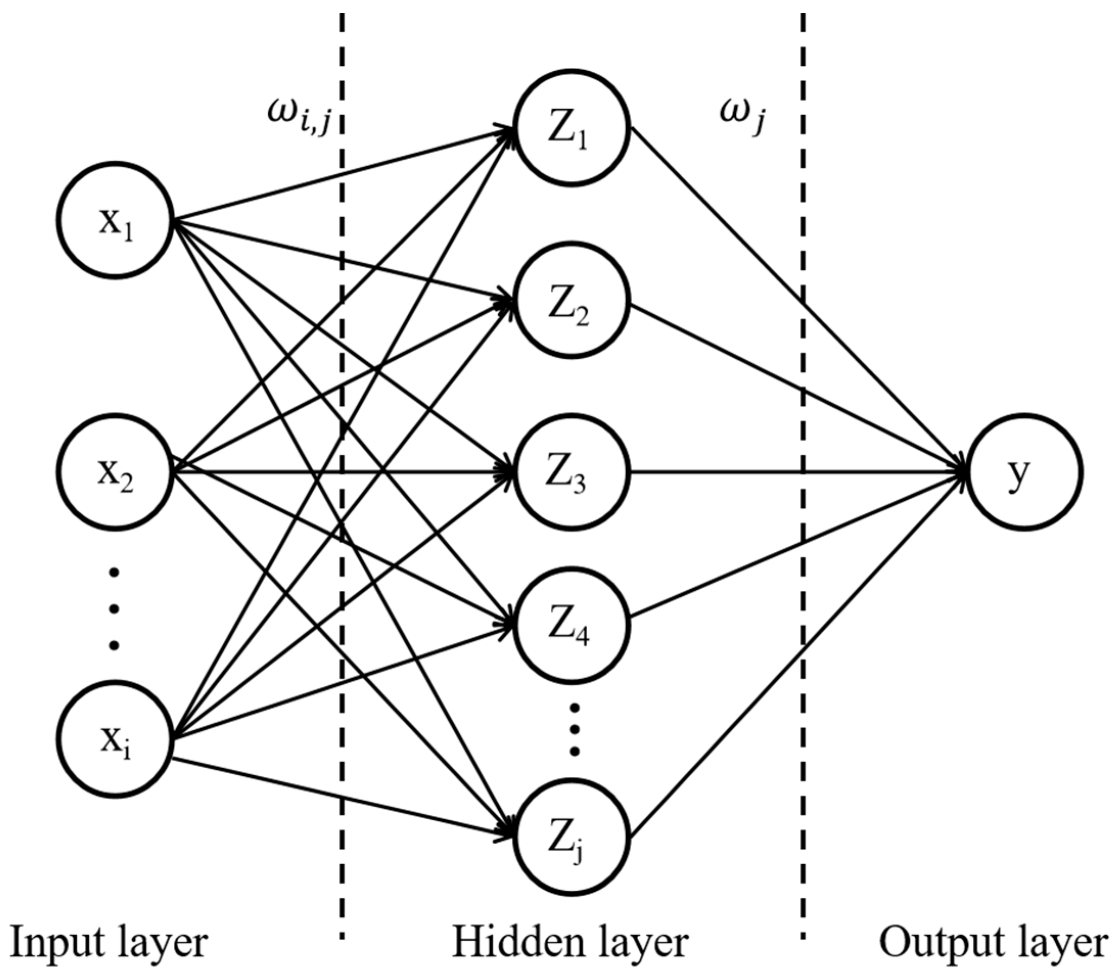
2.2.3. Backpropagation Neural Network

The backpropagation (BP) neural network is a concept proposed by scientists led by McClelland et al. in 1986 [28]. It is a multilayer feedforward neural network that is trained according to the error backpropagation algorithm and is one of the most widely used neural network models. The BP neural network consists of an input layer, a hidden layer, and an output layer, including forward propagation and backward propagation processes. Figure 2 shows the structure of the BP neural network.

In this study, a 9-layer neural network is used in the BP neural network, including an input layer, 7 hidden layers, and an output layer. The input layer has 5 nodes; the numbers of nodes in the 7 hidden layers are 64, 64, 32, 16, 16, 4, and 4; and 1 node is contained in the output layer. The activation function of the hidden layer is an ReLU, and the activation function of the output layer is linear.

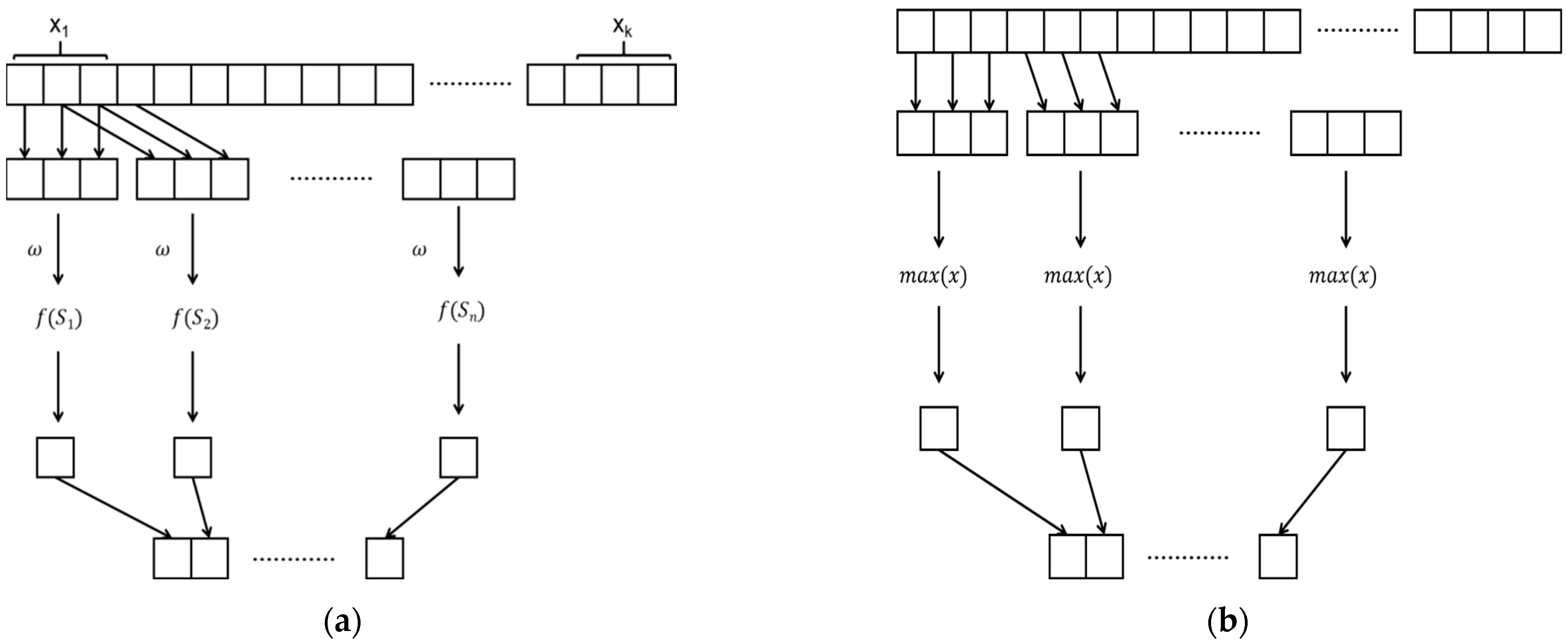
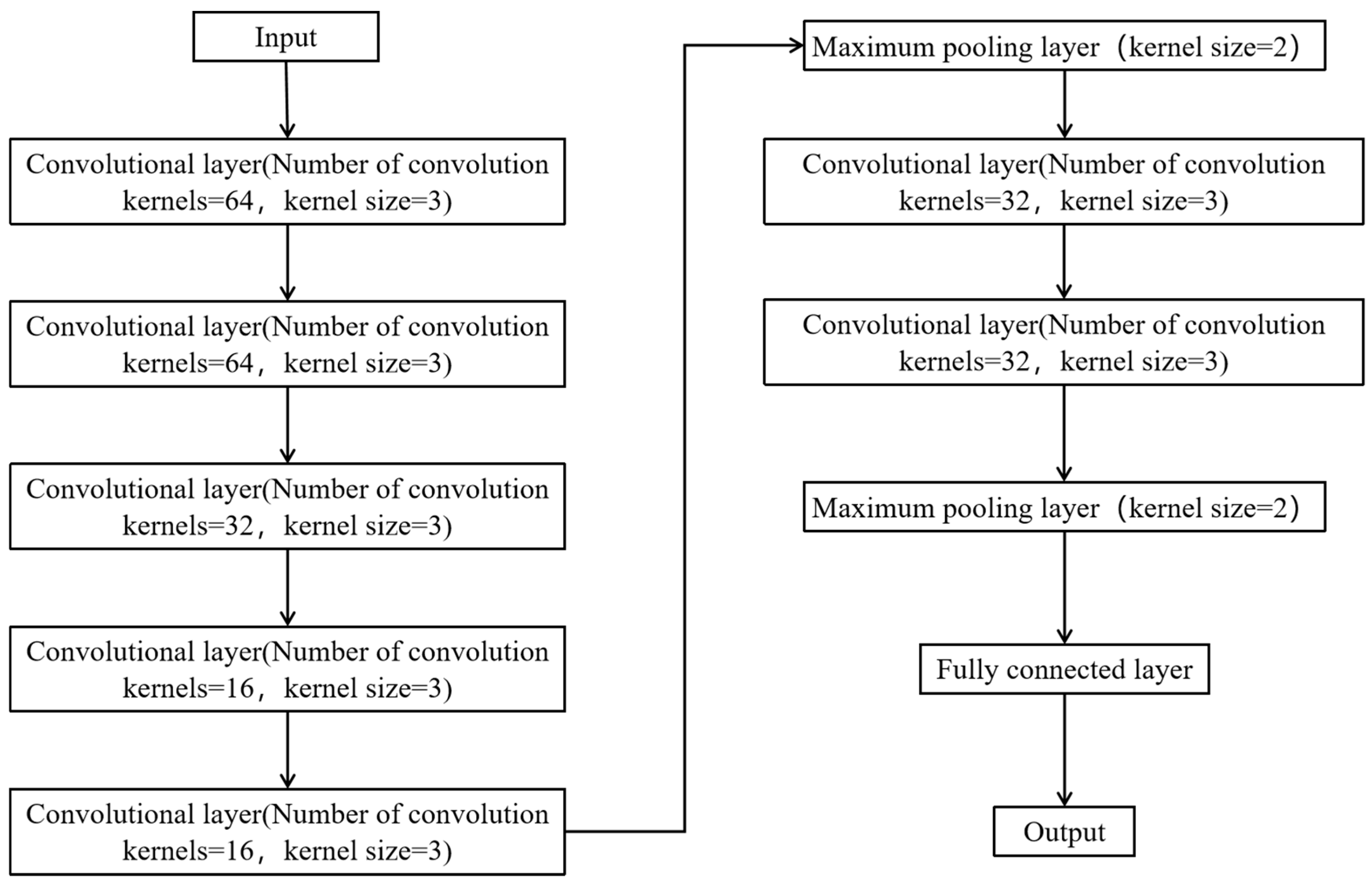
2.2.4. Convolutional Neural Network

The original convolutional neural network (CNN) was proposed by LeCun et al. in 1998 [29]. A CNN consists of three main parts: a convolutional layer, a maximum pooling layer, and a fully connected layer. It extracts local segments from a sequence according to a certain size window, and each subsequence is dotted with weights. The result of the dot product is subsequently combined into a new sequence, and the process is shown in Figure 3a.

The maximum pooling layer is mainly responsible for extracting features from the reinforced convolutional layer. Figure 3b shows a schematic diagram of the maximum pooling layer. The maximum pooling layer extracts local segments from the sequence according to a certain size window, takes the maximum value of each subsequence, and then combines them, which can reduce noise interference and improve the generalization ability of the model.

The input data are derived from data depicting contaminant concentration distributions obtained from experimentally validated CFD simulations. These data contain spatially continuous information and are well suited for processing with the CNN, which can automatically extract and learn spatial features from the data. We select a small filter size of 3, which captures sufficient local information while maintaining computational efficiency. Through multilayer convolutional operations, the model gradually extracts spatial features from low-to-high levels. Each convolutional layer is followed by a max pooling layer to reduce the size of the feature map and prevent overfitting. The max pooling layer extracts the maximum value from the local region, thereby preserving the most significant feature information. A final fully connected layer maps all the features to a single output value that represents the predicted contaminant concentration. A linear activation function is used to ensure that a linear relationship is maintained between the output value and the actual concentration value.

To determine the optimal configuration, we conducted extensive hyperparameter tuning experiments using various learning rates (0.001, 0.0005), batch sizes (64, 128), and training cycles (100, 200, 300). Ultimately, we selected the combination of a learning rate of 0.001, a batch size of 64, and a training period of 200, as this configuration yielded the lowest root mean square error (RMSE = 6.31 ppm), mean absolute error (MAE = 3.18 ppm), and mean absolute percentage error (MAPE = 8.33%) on the validation set. Additionally, we explored deeper and wider network architectures; however, while these adjustments increased the model capacity, they did not significantly improve the prediction accuracy and instead increased the risk of overfitting. Consequently, a 10-layer neural network is used in the CNN of this study, including 7 convolutional layers, 2 maximum pooling layers, and a fully connected layer, as shown in Figure 4. The activation function of the convolutional layer is an ReLU, and the activation function of the fully connected layer is linear. The final selected CNN architecture is considered to provide the best computational efficiency while ensuring optimal prediction performance.

2.3. Predictive Evaluation Indicators

This study uses the RMSE, MAE, MAPE, and R² metrics to evaluate the model. R² is a common metric that reflects the degree of fit of a model. The RMSE and MAE are used to measure the closeness between the predicted and observed values obtained for the test data. The MAPE is used to describe the relative error of the model. The RMSE, MAE, MAPE, and R² metrics are calculated as follows.

$$\mathrm{R}\mathrm{M}\mathrm{S}\mathrm{E}=\sqrt{{\displaystyle \frac{\sum _{\mathrm{i}=1}^{\mathrm{n}}({\mathrm{y}}_{\mathrm{i}}-{\mathrm{y}}_{\mathrm{i}}^{\prime }{)}^2}{\mathrm{n}}}}$$

(7)

$$\mathrm{M}\mathrm{A}\mathrm{E}={\displaystyle \frac{\sum _{\mathrm{i}=1}^{\mathrm{n}}\left|{\mathrm{y}}_{\mathrm{i}}-{\mathrm{y}}_{\mathrm{i}}^{\prime }\right|}{\mathrm{n}}}$$

(8)

$$\mathrm{M}\mathrm{A}\mathrm{P}\mathrm{E}={\displaystyle \frac{\sum _{\mathrm{i}=1}^{\mathrm{n}}\left|\frac{{\mathrm{y}}_{\mathrm{i}}-{\mathrm{y}}_{\mathrm{i}}^{\prime }}{{\mathrm{y}}_{\mathrm{i}}^{\prime }}\right|}{\mathrm{n}}}$$

(9)

$$R^2=1-{\displaystyle \frac{\sum _{i=1}^n({\mathrm{y}}_{\mathrm{i}}-{\mathrm{y}}_{\mathrm{i}}^{\prime }{)}^2}{\sum _{i=1}^n({\mathrm{y}}_{\mathrm{i}}^{\prime }-\overline{{\mathrm{y}}_{\mathrm{i}}^{\prime }}{)}^2}}$$

(10)

where y represents the predicted contamination concentration; y′ represents the true contamination concentration; and $\overline{{\mathrm{y}}_{\mathrm{i}}^{\prime }}$ represents the average of the true contamination concentration results.

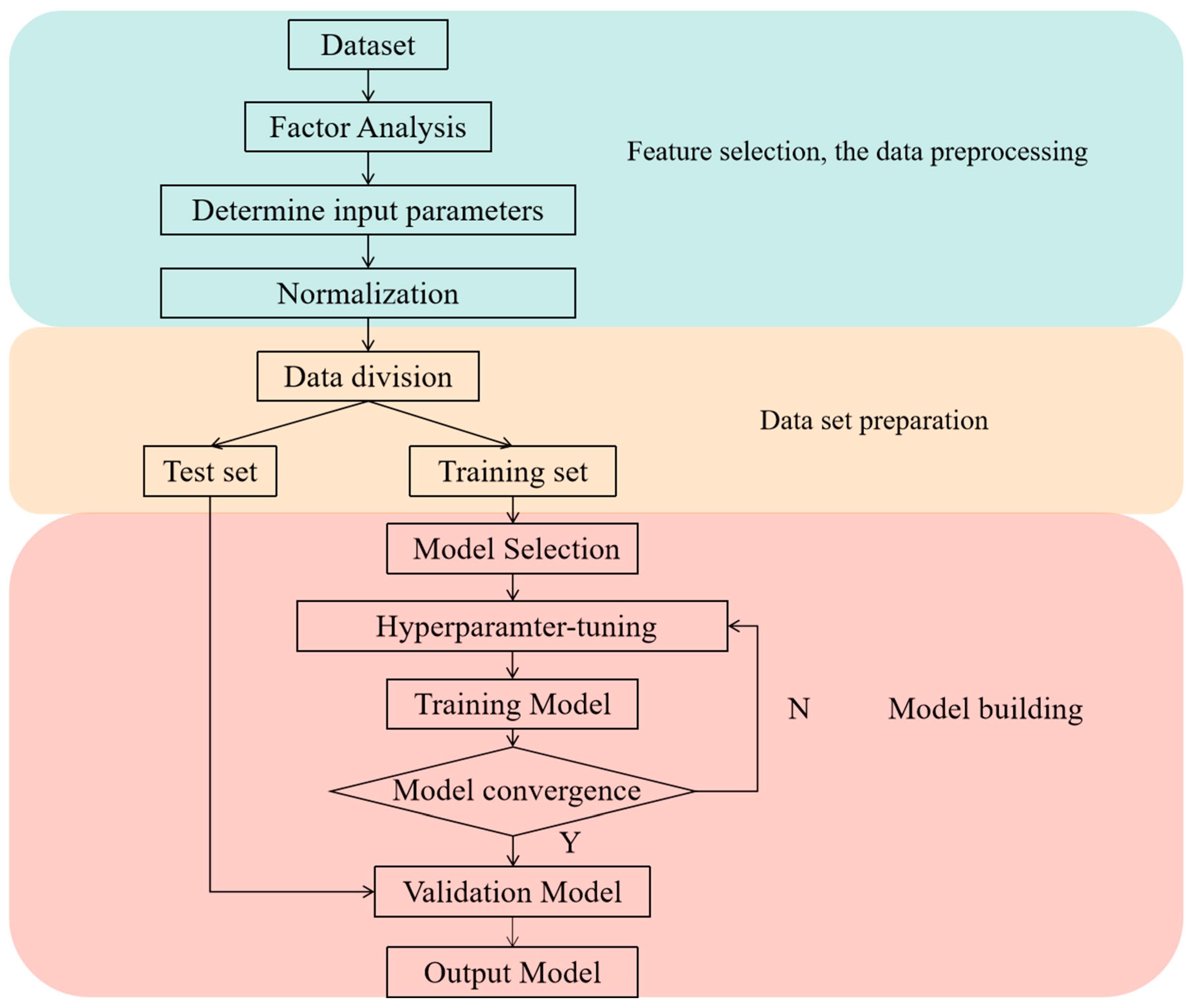
2.4. Machine Learning Model Construction Process

Figure 5 shows the flowchart of the machine learning model construction process. The construction of machine learning models consists of three parts: feature engineering, dataset preparation, and model building. First, the coordinates of each location in the room, the concentration of contamination at each location, and the amount of fresh air in the room are collected. Next, a factor analysis is performed. To reduce the number of required sensors, the room is divided into several areas, and the correlations among the contamination concentrations in different areas are analyzed to find the areas where the contamination concentrations need to be monitored. On the basis of the results of the factor analysis, the contamination concentration of the monitoring point, the fresh air volume of the room, and the coordinates of the predicted location are set as the input parameters, and the data are normalized by Equation (11).

$$\mathrm{X}\_\mathrm{s}\mathrm{t}\mathrm{a}\mathrm{n}\mathrm{d}\mathrm{a}\mathrm{r}\mathrm{d}\mathrm{i}\mathrm{z}\mathrm{e}\mathrm{d}={\displaystyle \frac{(\mathrm{X}-\mathsf{\mu })}{\mathsf{\sigma }}}$$

(11)

where $\mathrm{X}\_\mathrm{s}\mathrm{t}\mathrm{a}\mathrm{n}\mathrm{d}\mathrm{a}\mathrm{r}\mathrm{d}\mathrm{i}\mathrm{z}\mathrm{e}\mathrm{d}$ represents the data after normalization; $\mathrm{X}$ represents the original data; $\mathsf{\mu }$ represents the mean value of the original data; and $\mathsf{\sigma }$ represents the standard deviation of the data.

The preparation part of the dataset divides the dataset into a training set and a test set. The training set accounts for 70% of the dataset used to train the model, and the test set accounts for 30% of the dataset used to test the accuracy of the model. To assess the performance of machine learning models in accurately predicting indoor contaminant distributions, we used experimentally validated CFD simulation data. During data preparation, all the data points were randomly shuffled to ensure independence and representativeness between the training and test sets. Specifically, 70% of the data were allocated for training the model, whereas the remaining 30% were reserved for testing its accuracy. To account for potential temporal autocorrelation in contaminant concentrations, we generated data points for various periods during the CFD simulations to capture changes in contaminant levels over time and airflow patterns. However, preliminary analyses revealed that there was no significant temporal autocorrelation across the time points in the dataset used.

3. Dataset Acquisition

Many scholars have used CFD data to construct machine learning training and testing datasets [20,30]. As shown in the comparison experiments, CFD can provide accurate information about the flow distribution and concentration fields in the whole simulation domain. Therefore, this study uses validated CFD simulations to construct a dataset for training and testing machine learning methods via the constructed learning models. The data acquisition workflow is shown in Figure 6. First, a physical model is built on the basis of the actual arrangement of the ward. A mathematical model is then developed to mathematically obtain the indoor contamination distribution by selecting the RNG k-ε turbulence equation, the DO radiation equation, and the component transport equation. Once the model is established, tests are performed in a full-scale laboratory to obtain the indoor temperature, velocity, and contamination concentrations, which are compared with the simulated values to verify the accuracy of the model. Finally, the indoor contamination distribution is simulated with different numbers of air changes, and the simulation results are used as a dataset.

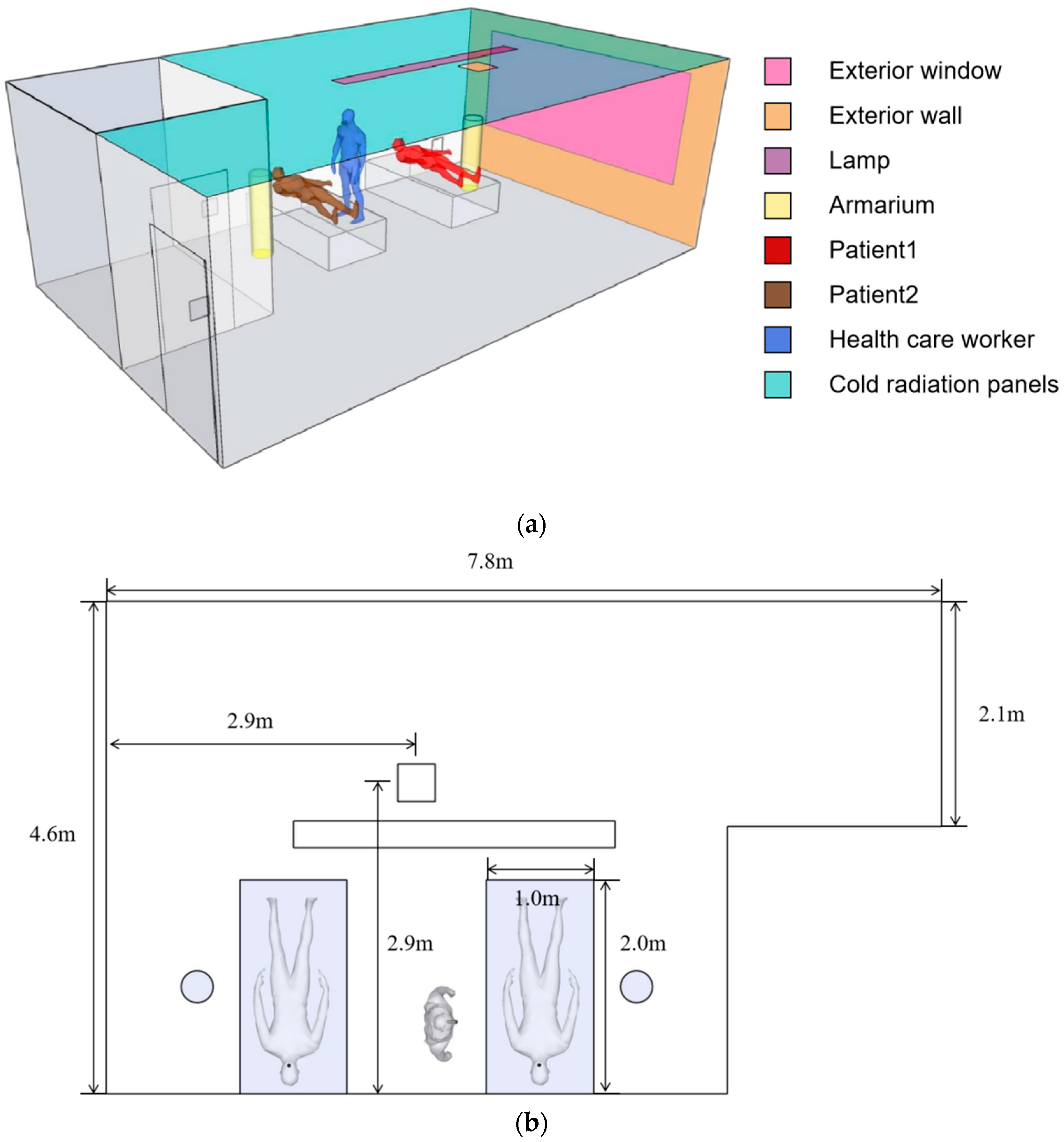
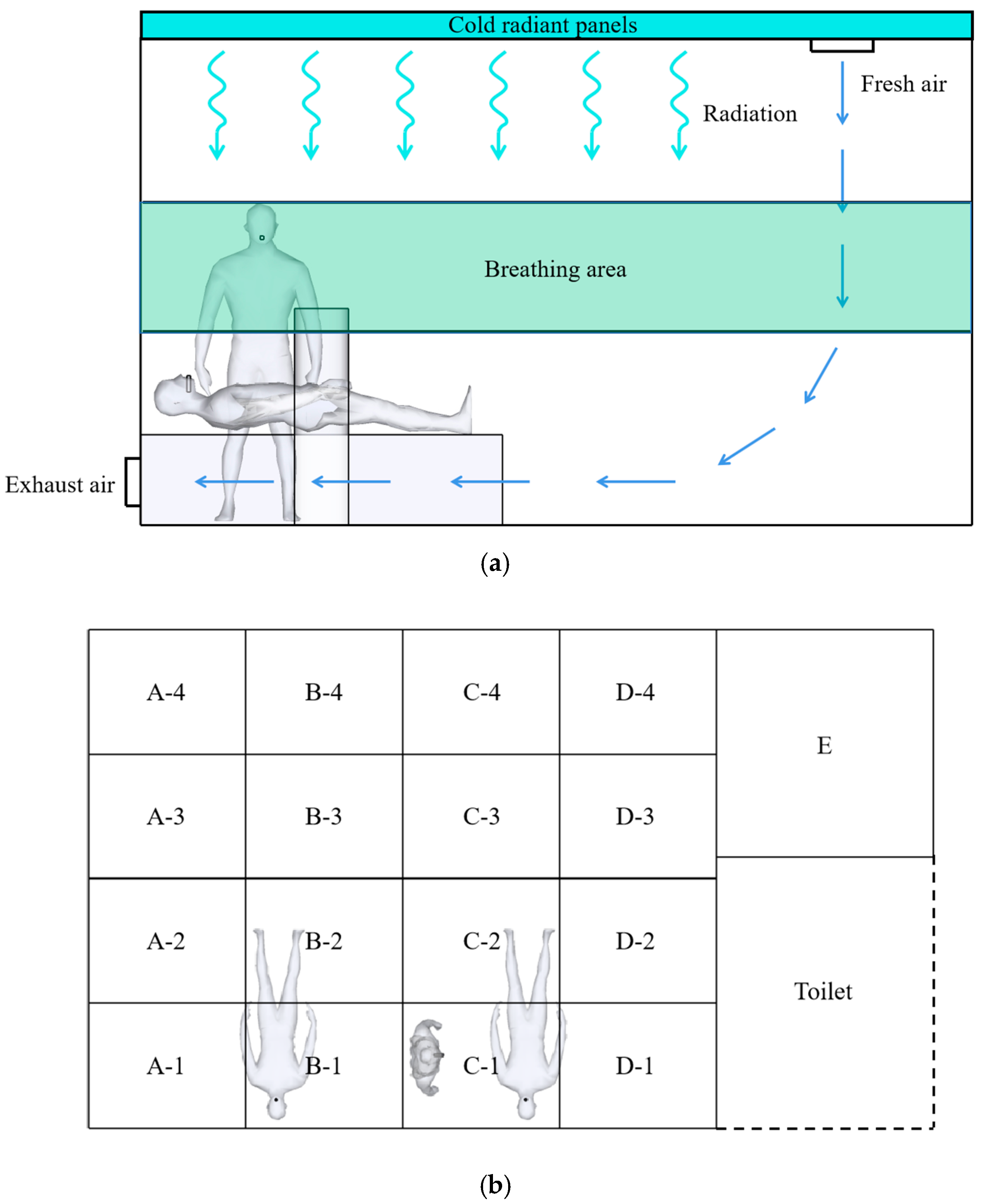
3.1. Indoor Environment Settings and Model Validation

In this study, we selected the RNG k-ε turbulence model to simulate airflow and contaminant distribution in a hospital ward. The RNG k-ε model improves the simulation accuracy for complex flow structures by refining certain assumptions found in the standard k-ε model, such as accounting for the effects of rotational and cyclonic flows. Specifically, the stability and computational efficiency of the RNG k-ε model in complex flow situations make it an ideal choice.

Although the shear stress transport (SST) model offers advantages for modeling flow near walls, particularly in regions with high shear rates, the RNG k-ε model is sufficiently accurate for our application scenario. This is due to the more homogeneous flow conditions in the wards and the absence of extreme shear flows. Furthermore, while large eddy simulation (LES) provides a more detailed representation of turbulence characteristics, it is computationally expensive, especially in 3D complex geometries. Considering that the main objective of this study is to quickly predict the contaminant distribution and that our resources are limited, the more computationally efficient RNG k-ε model is chosen.

A model of a negative pressure ward with applied radiant air conditioning is developed as a case study. As shown in Figure 7, the negative pressure ward is 7.8 m long, 4.6 m wide, and 2.7 m high. The interior is equipped with external walls, external windows, medical equipment, light bulbs, cold radiation panels, two patients, and one health care worker. Exterior walls, exterior windows, light bulbs, personnel, and medical equipment are used to simulate the heat gained by the room. Radiant cold panels were used to maintain the temperature of the room. Scholars have demonstrated the reliability of using carbon dioxide as a tracer gas, and this study uses carbon dioxide as a contaminant exhaled by patients [24,31]. The contaminants are exhaled from the mouths of two patients. In this work, the RNG k-ε equation is used to describe the contaminant distribution in the negative pressure ward. The maximum grid size of the model is 100 mm, the time step is set to 0.5 s, and the solver is set to SIMPLE.

Table 1. Boundary condition settings.

Surface	Boundary Conditions
Interior walls, floors	Wall; Adiabatic
Exterior walls	Wall; Heat flux: 35.89 W/m2
Exterior windows	Wall; Heat flux: 389 W/m2
Lamp	Wall; Heat flux: 133 W/m2
Patients and health care workers	Wall; Heat flux: 45 W/m2 [11]
Armarium	Wall; Heat flux: 389.71 W/m2
Mouth	Velocity-inlet: 0.88 m/s [32,33]; Temperature: 34 °C [34]
New air vent	Velocity-inlet: 1.13 m/s; Temperature: 18.64 °C
Ceiling	Wall; Temperature: 19 °C
Exhaust air vent	EA1, EA2, Velocity-inlet: −0.96 m/s; EA3 Velocity-inlet: −0.95 m/s [35]

shows the detailed settings of the boundary conditions.

To verify the accuracy of the CFD results, a laboratory is established according to the CFD model, and the laboratory is shown in Figure 8. Previous studies have compared the computational results of the CFD model with experimental results and demonstrated the reliability of the model [36].

3.2. Preparing the Dataset

The number of air changes has an important effect on the indoor contamination concentration [37], and changes in the number of air changes will result in changes in the indoor contamination distribution. The number of air changes in the ward is easily affected by various factors. For example, the opening of a room door will cause a change in pressure in the room [38], which will result in a change in the number of air changes in the room. Moreover, a fresh air unit needs to provide fresh air to several rooms, and a change in the number of air changes in one room will lead to a change in the number of air changes in several rooms. As a result, the number of air changes in the room is difficult to maintain in a steady state. Therefore, to evaluate the ability of the machine learning models to predict indoor contamination distributions accurately, indoor contamination distributions are simulated under different numbers of air changes using CFD, and the dataset obtained from the CFD simulations is used to train and test the machine learning models.

A total of 22 scenarios are simulated, and the contamination distribution data in the height range of 1.3–1.7 m are used for the analysis of regional contamination concentrations, as well as the training and testing of the machine learning models. Scenarios 1–10 present the indoor contamination distributions when the indoor flow field is stable. Scenarios 11–22 present the indoor contamination distributions when the indoor flow field is changed. When the indoor flow field changes, the indoor contamination distribution is obtained every 5 min, and the indoor contamination distribution is recorded for one hour in total. The data obtained from Scenarios 1 to 10 are used to analyze the correlations among the contamination concentrations in different areas, and the data obtained from Scenarios 11 to 19 are used as the dataset for training the machine learning models, with a total of 90,720 points of data. The data obtained from Scenarios 20 to 22 are utilized as the test set to evaluate the accuracy of the machine learning models, with a total of 30,240 data points.

Table 2. Scenario settings.

Scenario	Air Changes Under a Steady State	Air Changes After State Changes	Scenario	Air Changes Under a Steady State	Air Changes After State Changes
Scenario 1	3	3	Scenario 12	12	6
Scenario 2	4	4	Scenario 13	12	9
Scenario 3	5	5	Scenario 14	9	3
Scenario 4	6	6	Scenario 15	9	6
Scenario 5	7	7	Scenario 16	9	12
Scenario 6	8	8	Scenario 17	6	3
Scenario 7	9	9	Scenario 18	6	9
Scenario 8	10	10	Scenario 19	6	12
Scenario 9	11	11	Scenario 20	3	6
Scenario 10	12	12	Scenario 21	3	9
Scenario 11	12	3	Scenario 22	3	12

shows the detailed scenario settings.

4. Results and Discussion

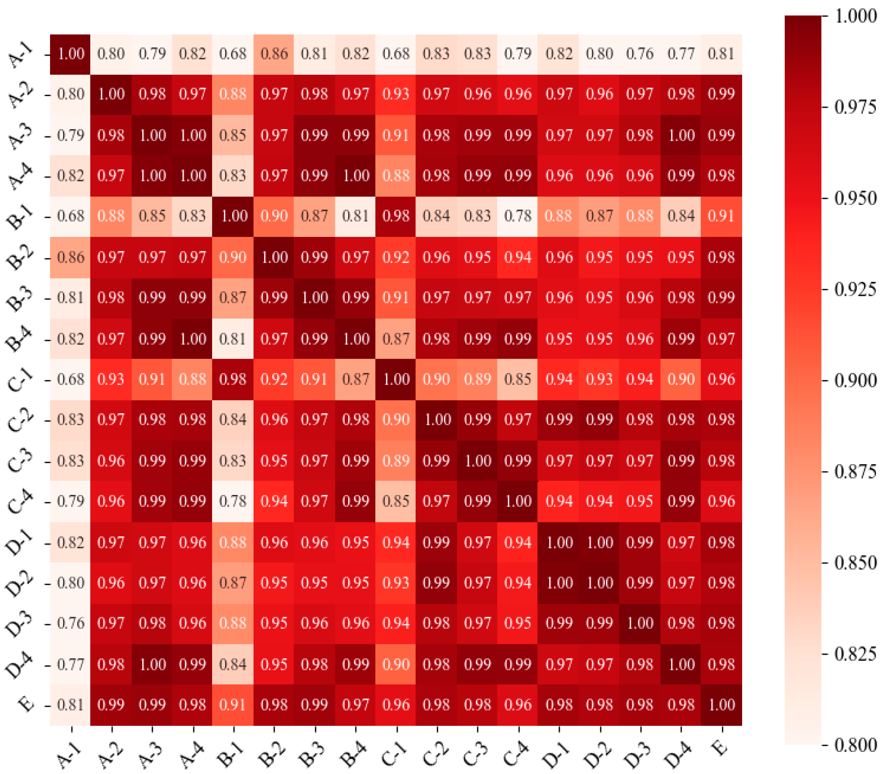
4.1. Regional Contamination Correlation Analysis

The breathing zone for medical personnel is at 1.3–1.7 m, so only the distributions of the indoor contamination concentrations at 1.3–1.7 m in the room are considered [11]. To analyze the indoor contamination concentration distributions in different areas more accurately, the room is divided into 17 boxes, as shown in Figure 9.

Figure 10 shows the correlation analysis of the contamination concentrations in different regions. The figure shows that the Pearson coefficients are greater than 0.8 for all the indoor areas. There are strong correlations between the contamination concentrations in the E region and those in all the indoor regions. The correlations between the contamination concentrations in the central area of the room and other indoor areas are not as strong as those involving the E area. This is because the center area is closer to the fresh air outlet, resulting in a low contamination concentration in the area; thus, the contamination concentration in this area cannot reflect the actual contamination concentration in the room.

To accurately predict the indoor contamination distributions, the contamination concentrations in area E are monitored. Moreover, on the basis of the correlation analysis results, the sensors were arranged in areas A-1, B-1, C-1, C-4, and B-4 to analyze the influence of the sensor arrangement on the prediction accuracy. Figure 11 shows the sensor arrangement locations.

Table 3. Case settings.

Case	Sensor Arrangement Area	Sensor Number
Case 1	E	Sensor 1
Case 2	E,A-1	Sensors 1–2
Case 3	E,A-1,B-1	Sensors 1–3
Case 4	E,A-1,B-1,C-1	Sensors 1–4
Case 5	E,A-1,B-1,C-1,C-4	Sensors 1–5
Case 6	E,A-1,B-1,C-1,C-4,B-4	Sensors 1–6

shows the case settings. The input parameters of the model are the coordinate positions of the prediction points, including X-axis and Y-axis coordinates, the pollution concentration of the monitoring points, and the number of room air changes.

Figure 12 shows the forecast evaluation metrics for different cases. As shown in Figure 12, the model accuracy increases when the number of sensors is increased from one to two. Compared with those of Case 1, the RMSE, MAE, and MAPE of Case 2 are reduced by 19.54%, 17.57%, and 17.67%, respectively. However, when the sensors continue to be added, the model accuracy decreases. Compared with those of Case 2, the RMSE, MAE, and MAPE of Case 6 increase by 10.63%, 12.71%, and 17.84%, respectively. This finding shows that increasing the sensor arrangement can improve the model accuracy, but too many arrangements of sensors are not effective in improving the model accuracy and even lead to the degradation of the model accuracy, so a reasonable arrangement of sensors in the ward is needed.

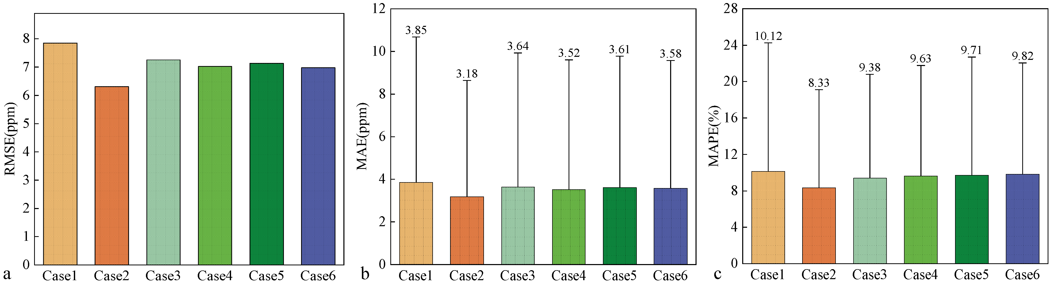
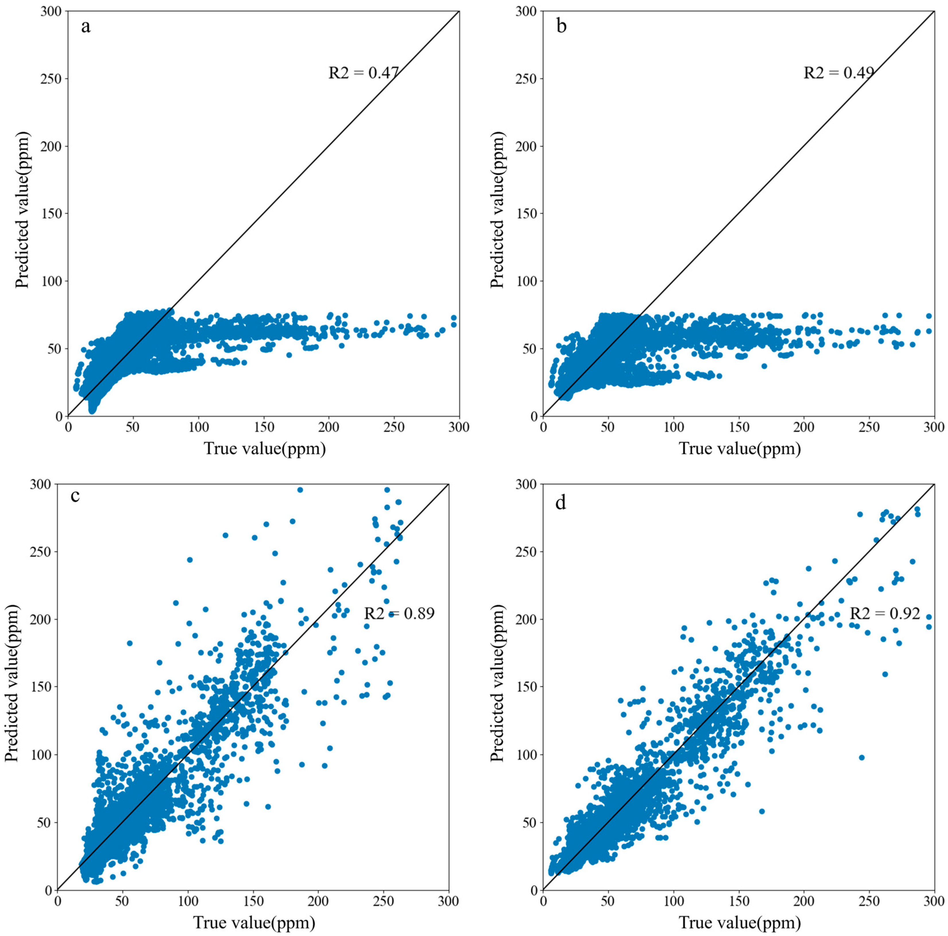
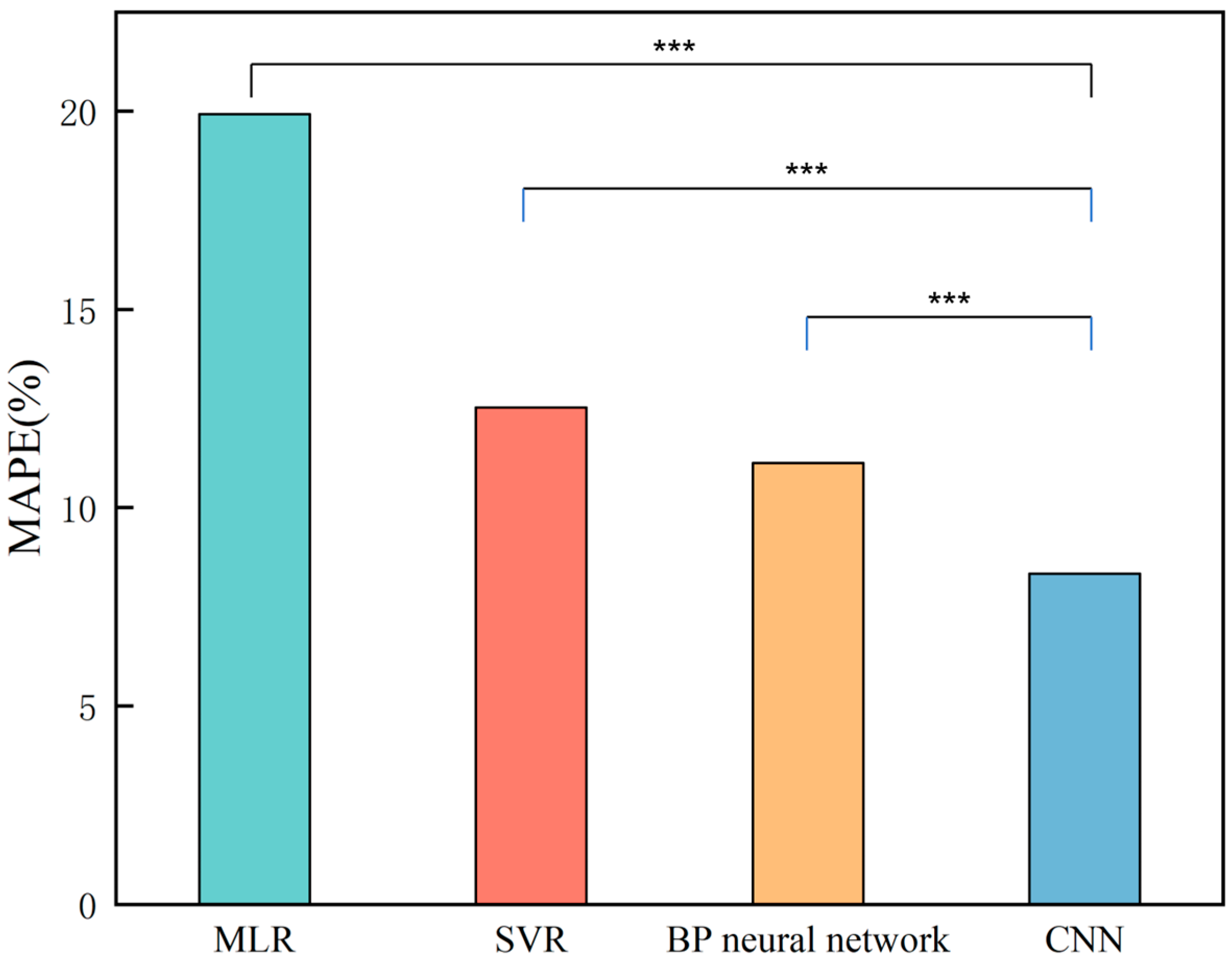
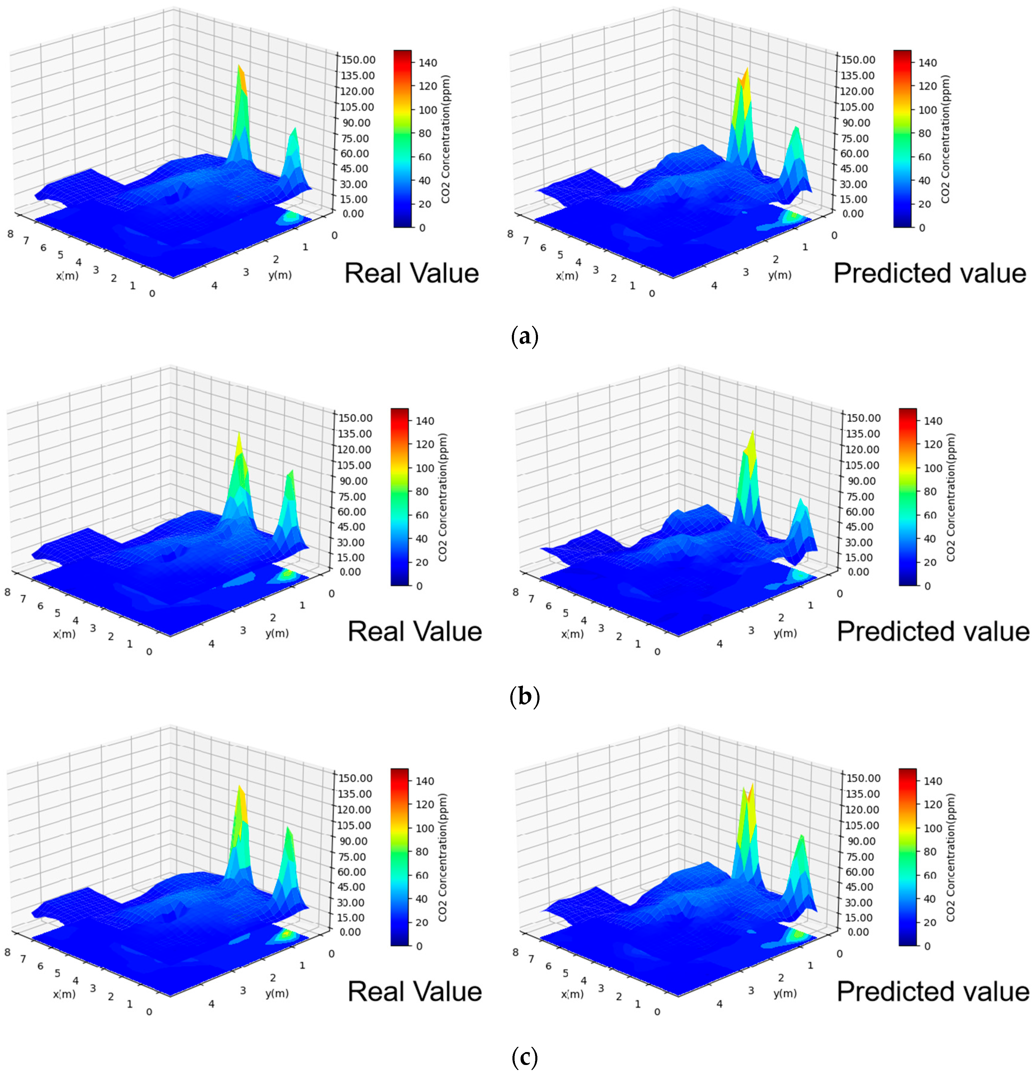
4.2. Indoor Contamination Concentration Prediction

The MLR model, SVR model, BP neural network, and CNN are trained on the training set and then tested on the test set. Figure 13 shows the prediction results of the four models. The figure shows that MLR and SVR have higher prediction accuracies at lower contamination concentrations but lower prediction accuracies in areas with higher contamination concentrations, and the R² values of these two models are 0.47 and 0.49, respectively. The BP neural network and CNN can ensure higher accuracy in different concentration ranges, and the R² values of these two models are 0.89 and 0.91, respectively.

Figure 14 shows the comparison between the RMSE and MAE values of different models. The RMSE and MAE values of MLR are the highest among all four models, with values of 15.73 ppm and 7.61 ppm, respectively. The RMSE of the SVR model is similar to that of the MLR model at 15.4 ppm. Compared with that of MLR, the MAE value is reduced by 24.18%. This indicates that the overall prediction effect of SVR is better than that of the linear model, but for outlier prediction, the performances of SVR and MLR are basically the same. The RMSE and MAE values of both the BP neural network and the CNN are lower than those of SVR and MLR. Compared with those of SVR, the RMSE and MAE of the BP neural network are 50.74% and 30.77% lower, respectively. The CNN has the best performance among the four models, with RMSE and MAE values of 6.31 ppm and 3.18 ppm, respectively, and compared with those of the BP neural network, these values decrease by 16.80% and 20.47%, respectively. This finding indicates that the best prediction results can be obtained by using a CNN for indoor contamination concentration prediction. The results show that among the four machine learning models, the BP neural network and CNN can better fit the variation patterns of indoor contamination and make effective indoor contamination predictions.

Figure 15 shows the MAPE values of the different models. The figure shows that MLR has the worst prediction effect, with an MAPE of 19.92%. The MAPEs of the SVR and BP neural networks are basically the same at 12.52% and 11.13%, respectively. The CNN performs best among the four models, with an MAPE of 8.33%. Comparative analysis revealed that the CNN reduced the MAPE by 58.18%, 33.47%, and 25.15% compared with the MLR, SVR, and BP neural network, respectively.

To assess the performance differences among various machine learning models more accurately, we not only presented the average performance metrics (e.g., RMSE, MAE, MAPE, and R²) using bar charts (see Figure 14 and Figure 15) but also verified whether these differences were statistically significant through appropriate statistical tests. For each performance metric, we conducted a paired-samples t-test when the data met the assumption of a normal distribution or a Wilcoxon signed-rank test when the data did not meet this assumption. The findings demonstrate that, in most cases, the CNN model has significant advantages over the other models (MLR, SVR, and BP neural network) across all the performance metrics.

The abovementioned findings demonstrate that the CNN has the best prediction effect. To observe the prediction effect of the CNN when the indoor contamination changes, the CNN is used to predict the indoor contamination distributions for Case 22 at 20 min, 40 min, and 60 min, as shown in Figure 16. The figure shows that the CNN prediction results are very similar to the actual contamination distribution. The CNN not only accurately predicts the indoor contamination distribution but also predicts the increase in the contamination concentration near the source, which is important for accurately predicting the risk of indoor human infection.

4.3. Discussion

Figure 12 shows that increasing the sensor arrangement can improve the model accuracy, but too many sensors cannot effectively improve the model accuracy and can even lead to a decrease in the model accuracy. Similar findings were reported by Ren & Cao [30], who reported that adding sensors did not necessarily improve model accuracy. This is due to the existence of correlations between contamination concentrations in different regions. When the input variables are correlated, the covariance problem of the input variables leads to a decrease in the generalization ability of the model [39]. Therefore, when determining the input parameters, a correlation analysis of the input parameters should be performed to avoid inappropriate input parameters leading to a decrease in model accuracy.

Beyond sensor deployment, the choice of machine learning algorithms further determines the prediction accuracy. A comprehensive comparison of the four models (MLR, SVR, the BP neural network, and the CNN) across the MAE, MAPE, R², and RMSE metrics (Figure 13, Figure 14 and Figure 15) reveals significant performance disparities. Across the four indicators, the MLR has the worst values, indicating that it is inappropriate to apply the MLR to indoor contamination concentration prediction. This is because indoor contamination concentrations vary nonlinearly, and MLR cannot accurately describe nonlinear variations [24]. Figure 13 shows that SVR has high prediction accuracy for data-dense areas, but its prediction results for data-sparse areas show large deviations. This finding is similar to that of Du et al., who suggested that SVR does not effectively predict data-sparse regions [37]. Figure 16 shows that indoor contamination tends to form aggregates near patients, resulting in a small number of areas with much higher contamination concentrations than other areas. Therefore, when SVR is used to predict indoor contamination distributions, the contamination concentrations in these areas are not accurately predicted. Figure 13 shows that the BP neural network is also able to predict data-sparse regions more accurately than SVR does. Moreover, the BP neural network is significantly better than SVR in terms of its RMSE, MAE, and R² values, indicating that the BP neural network is better than SVR with respect to contamination prediction accuracy. Although the BP neural network can extract the contamination distribution pattern from the data, the indoor contamination distribution pattern is very complex, and the BP neural network cannot fully learn the hidden knowledge contained in the data. The CNN can extract features from multidimensional spatial data and identify changing patterns more accurately [40]. Therefore, the CNN is better than the BP neural network for the prediction of indoor contamination.

Although the results of Case 22 show that the CNN model has high accuracy in time series prediction, a single scenario may not comprehensively represent the model’s performance across various dynamic conditions. Therefore, in future studies, both the number and diversity of test scenarios should be increased to further validate the model’s generalizability.

For example, additional representative scenarios (e.g., Case 5, Case 14, and Case 30) can be selected from the existing CFD simulation data, and the same evaluation method can be used for a comprehensive comparison. This approach will not only help identify the potential limitations of the model under specific conditions but also offer more comprehensive support for a range of complex scenarios that may occur in real-world applications.

5. Conclusions

In this study, four machine learning methods (MLR, SVR, a BP neural network, and a CNN) are applied to hospital ward contamination prediction, and their prediction results are compared and analyzed. The results of this study are as follows.

(1) Correlations are observed between the contamination concentrations in different areas in hospital wards, and when monitoring hospital ward contamination concentrations, representative areas should be selected.

(2) Machine learning models achieve accurate spatiotemporal prediction of hospital ward contaminant concentration distributions with strategically limited sensor data inputs. Excessive sensor inputs not only fail to enhance model prediction fidelity but also may induce performance degradation through overfitting mechanisms.

(3) Not all machine learning models exhibit effective predictive capabilities for contamination distributions in hospital wards. When MLR and SVR are used, their R² values are 0.47 and 0.49, respectively, indicating that they cannot effectively predict hospital ward contamination distributions. The BP neural network and CNN can predict hospital ward contamination in cases with limited monitoring points. Among them, the CNN has the best prediction effect, with R², RMSE, MAE, and MAPE values of 0.92, 6.31 ppm, 3.18 ppm, and 8.33%, respectively. Compared with those of the BP neural network, the RMSE, MAE, and MAPE of the CNN decrease by 16.80%, 20.47%, and 25.15%, respectively. Therefore, the use of a CNN to rapidly predict contamination distributions in hospital wards is recommended.

References

1. Riley, E.C.; Murphy, G.; Riley, R.L. Airborne spread of measles in a suburban elementary school. Am. J. Epidemiol. 1978, 107, 421–432. [Google Scholar] [CrossRef] [PubMed]
2. Han, K.-T.; Kim, S. Impact of COVID-19 on nurse staffing levels and healthcare-associated infections in medical institutions: A retrospective cohort study. Sci. Rep. 2025, 15, 13351. [Google Scholar] [CrossRef] [PubMed]
3. Ren, C.; Wang, J.; Feng, Z.; Kim, M.K.; Haghighat, F.; Cao, S.-J. Refined design of ventilation systems to mitigate infection risk in hospital wards: Perspective from ventilation openings setting. Environ. Pollut. 2023, 333, 122025. [Google Scholar] [CrossRef] [PubMed]
4. Yan, S.; Wang, L.L.; Birnkrant, M.J.; Zhai, J.; Miller, S.L. Evaluating SARS-CoV-2 airborne quanta transmission and exposure risk in a mechanically ventilated multizone office building. Build. Environ. 2022, 219, 109184. [Google Scholar] [CrossRef]
5. Mei, D.; Duan, W.; Li, Y.; Li, J.; Chen, W. Evaluating risk of SARS-CoV-2 infection of the elderly in the public bus under personalized air supply. Sustain. Cities Soc. 2022, 84, 104011. [Google Scholar] [CrossRef]
6. Liu, Z.; Yao, G.; Li, Y.; Huang, Z.; Jiang, C.; He, J.; Wu, M.; Liu, J.; Liu, H. Bioaerosol distribution characteristics and potential SARS-CoV-2 infection risk in a multi-compartment dental clinic. Build. Environ. 2022, 225, 109624. [Google Scholar] [CrossRef]
7. Fennelly, K.P.; Nardell, E.A. The relative efficacy of respirators and room ventilation in preventing occupational tuberculosis. Infect. Control Hosp. Epidemiol. 1998, 19, 754–759. [Google Scholar] [CrossRef]
8. Zhang, S.; Lin, Z. Dilution-based evaluation of airborne infection risk—Thorough expansion of Wells-Riley model. Build. Environ. 2021, 194, 107674. [Google Scholar] [CrossRef]
9. Aganovic, A.; Cao, G.; Kurnitski, J.; Melikov, A.; Wargocki, P. Zonal modeling of air distribution impact on the long-range airborne transmission risk of SARS-CoV-2. Appl. Math. Model. 2022, 112, 800–821. [Google Scholar] [CrossRef]
10. Fisk, W.J.; Seppänen, O.; Faulkner, D.; Huang, J. Economic benefits of an economizer system: Energy savings and reduced sick leave. ASHRAE Trans. 2005, 111, 673–679. [Google Scholar]
11. Lu, Y.; Oladokun, M.; Lin, J.Z. Reducing the exposure risk in hospital wards by applying stratum ventilation system. Build. Environ. 2020, 183, 107204. [Google Scholar] [CrossRef]
12. Cho, J. Investigation on the contaminant distribution with improved ventilation system in hospital isolation rooms: Effect of supply and exhaust air diffuser configurations. Appl. Therm. Eng. 2018, 148, 208–218. [Google Scholar] [CrossRef]
13. Wei, S.; Wu, W.; Jeon, G.; Ahmad, A.; Yang, X. Improving resolution of medical images with deep dense convolutional neural network. Concurr. Comput. Pract. Exp. 2020, 32, e5084. [Google Scholar] [CrossRef]
14. Mishra, J.; Goyal, S. An effective automatic traffic sign classification and recognition deep convolutional networks. Multimed. Tools Appl. 2022, 81, 18915–18934. [Google Scholar] [CrossRef]
15. Luo, Q.; Ou, C.; Hang, J.; Luo, Z.; Yang, H.; Yang, X.; Zhang, X.; Li, Y.; Fan, X. Role of pathogen-laden expiratory droplet dispersion and natural ventilation explaining a COVID-19 outbreak in a coach bus. Build. Environ. 2022, 220, 109160. [Google Scholar] [CrossRef] [PubMed]
16. Zhang, S.; Niu, D.; Lu, Y.; Lin, Z. Contaminant removal and contaminant dispersion of air distribution for overall and local airborne infection risk controls. Sci. Total Environ. 2022, 833, 155173. [Google Scholar] [CrossRef] [PubMed]
17. Portal-Porras, K.; Fernandez-Gamiz, U.; Zulueta, E.; Irigaray, O.; Garcia-Fernandez, R. Hybrid LSTM+CNN architecture for unsteady flow prediction. Mater. Today Commun. 2023, 35, 106281. [Google Scholar] [CrossRef]
18. Portal-Porras, K.; Fernandez-Gamiz, U.; Zulueta, E.; Ballesteros-Coll, A.; Zulueta, A. CNN-based flow control device modelling on aerodynamic airfoils. Sci. Rep. 2022, 12, 8205. [Google Scholar] [CrossRef]
19. Bhatnagar, S.; Afshar, Y.; Pan, S.; Duraisamy, K.; Kaushik, S. Prediction of aerodynamic flow fields using convolutional neural networks. Comput. Mech. 2019, 64, 525–545. [Google Scholar] [CrossRef]
20. Tian, X.; Cheng, Y.; Lin, Z. Modelling indoor environment indicators using artificial neural network in the stratified environments. Build. Environ. 2022, 208, 108581. [Google Scholar] [CrossRef]
21. Liu, G.; Ren, L.; Qu, G.; Zhang, Y.; Zang, X. Fast prediction model of three-dimensional temperature field of commercial complex for entrance-atrium temperature regulation. Energy Build. 2022, 273, 112380. [Google Scholar] [CrossRef]
22. Warey, A.; Kaushik, S.; Khalighi, B.; Cruse, M.; Venkatesan, G. Data-driven prediction of vehicle cabin thermal comfort: Using machine learning and high-fidelity simulation results. Int. J. Heat Mass Transf. 2020, 148, 119083. [Google Scholar] [CrossRef]
23. Pang, S.; Song, L.; Kasabov, N. Correlation-aided support vector regression for forex time series prediction. Neural Comput. Appl. 2011, 20, 1193–1203. [Google Scholar] [CrossRef]
24. Gao, K.; Mei, G.; Piccialli, F.; Cuomo, S.; Tu, J.; Huo, Z. Julia language in machine learning: Algorithms, applications, and open issues. Comput. Sci. Rev. 2020, 37, 100254. [Google Scholar] [CrossRef]
25. Drucker, H.; Burges, C.J.; Kaufman, L.; Smola, A.; Vapnik, V. Support vector regression machines. In Advances in Neural Information Processing Systems, 9; MIT Press: Cambridge, MA, USA, 1996. [Google Scholar]
26. Malik, A.; Tikhamarine, Y.; Souag-Gamane, D.; Kisi, O.; Pham, Q.B. Support vector regression optimized by meta-heuristic algorithms for daily streamflow prediction. Stoch. Environ. Res. Risk Assess. 2020, 34, 1755–1773. [Google Scholar] [CrossRef]
27. Wang, X.; Wang, Y. A Hybrid Model of EMD and PSO-SVR for Short-Term Load Forecasting in Residential Quarters. Math. Probl. Eng. 2016, 2016, 1–10. [Google Scholar] [CrossRef]
28. McClelland, J.L.; Rumelhart, D.E.; PDP Research Group. Parallel Distributed Processing; MIT Press: Cambridge, MA, USA, 1986; Volume 2, pp. 20–21. [Google Scholar]
29. Lecun, Y.; Bottou, L.; Bengio, Y.; Haffner, P. Gradient-based learning applied to document recognition. Proc. IEEE 1998, 86, 2278–2324. [Google Scholar] [CrossRef]
30. Ren, J.; Cao, S.J. Incorporating online monitoring data into fast prediction models towards the development of artificial intelligent ventilation systems. Sustain. Cities Soc. 2019, 47, 101498. [Google Scholar] [CrossRef]
31. Richardson, E.T.; Morrow, C.D.; Kalil, D.B.; Bekker, L.G.; Wood, R. Shared air: A renewed focus on ventilation for the prevention of tuberculosis transmission. PLoS ONE 2014, 9, e96334. [Google Scholar] [CrossRef]
32. Qian, H.; Li, Y.; Nielsen, P.V.; Hyldgaard, C.E.; Wong, T.W.; Chwang, A.T. Dispersion of exhaled droplet nuclei in a two-bed hospital ward with three different ventilation systems. Indoor Air 2006, 16, 111–128. [Google Scholar] [CrossRef]
33. Olmedo, I.; Nielsen, P.V.; Ruiz de Adana, M.; Jensen, R.L.; Grzelecki, P. Distribution of exhaled contaminants and personal exposure in a room using three different air distribution strategies. Indoor Air 2012, 22, 64–76. [Google Scholar] [CrossRef]
34. Liu, F.; Zhang, C.; Qian, H.; Zheng, X.; Nielsen, P.V. Direct or indirect exposure of exhaled contaminants in stratified environments using an integral model of an expiratory jet. Indoor Air 2019, 29, 591–603. [Google Scholar] [CrossRef] [PubMed]
35. Ministry of Housing and Urban-Rural Development of the People’s Republic of China. Code for Design of General Hospital; China Planning Press: Beijing, China, 2015. [Google Scholar]
36. Zhou, C.G.; Ding, Y.F.; Ye, L.F. Study on infection risk in a negative pressure ward under different fresh airflow patterns based on a radiation air conditioning system. Environ. Sci. Pollut. Res. 2024, 31, 14135–14155. [Google Scholar] [CrossRef] [PubMed]
37. Du, B.; Lund, P.D.; Wang, J.; Kolhe, M.; Hu, E. Comparative study of modelling the thermal efficiency of a novel straight through evacuated tube collector with MLR, SVR, BP and RBF methods. Sustain. Energy Technol. Assess. 2021, 44, 101029. [Google Scholar] [CrossRef]
38. Hang, J.; Li, Y.; Ching, W.; Wei, J.; Jin, R.; Liu, L.; Xie, X. Potential airborne transmission between two isolation cubicles through a shared anteroom. Build. Environ. 2015, 89, 264–278. [Google Scholar] [CrossRef]
39. Cheng, P.; Chen, D.; Wang, J. Research on prediction model of thermal and moisture comfort of underwear based on principal component analysis and Genetic Algorithm–Back Propagation neural network. Int. J. Nonlinear Sci. Numer. Simul. 2021, 22, 607–619. [Google Scholar] [CrossRef]
40. Kwon, S.; Park, G.; Jang, Y.; Cho, J.; Chu, M.-G.; Min, B. Determination of oil well placement using convolutional neural network coupled with robust optimization under geological uncertainty. J. Pet. Sci. Eng. 2021, 201, 108118. [Google Scholar] [CrossRef]
Figure 1. Research framework.
Buildings 15 01828 g001
Figure 2. BP neural network structure.
Buildings 15 01828 g002
Figure 3. CNN schematic diagram. (a) Schematic diagram of the convolutional layer; (b) Schematic diagram of the maximum pooling layer.
Buildings 15 01828 g003
Figure 4. CNN structure.
Buildings 15 01828 g004
Figure 5. Flowchart of the machine learning model construction process.
Buildings 15 01828 g005
Figure 6. Data acquisition process.
Buildings 15 01828 g006
Figure 7. Physical model of the negative pressure ward: (a) negative pressure ward layout and (b) negative pressure ward size.
Buildings 15 01828 g007
Figure 8. Laboratory layout.
Buildings 15 01828 g008
Figure 9. Indoor zone divisions. (a) Breathing zone division; (b) Plane zone division.
Buildings 15 01828 g009
Figure 10. Pearson correlation coefficients for different regions.
Buildings 15 01828 g010
Figure 11. Division of the prediction area.
Buildings 15 01828 g011
Figure 12. Predictive evaluation indicators of different cases: (a) RMSE of different cases, (b) MAE of different cases, and (c) MAPE of different cases.
Buildings 15 01828 g012
Figure 13. Prediction results of the machine learning models: (a) MLR; (b) SVR; (c) BPNN; (d) CNN.
Buildings 15 01828 g013
Figure 14. RMSE and MAE histograms of the machine learning models (*** p < 0.001).
Buildings 15 01828 g014
Figure 15. MAPE histograms of the machine learning models (*** p < 0.001).
Buildings 15 01828 g015
Figure 16. Comparison between the CNN-predicted and real values: (a) 20-min contamination distribution; (b) 40-min contamination distribution; and (c) 60-min contamination distribution.
Buildings 15 01828 g016