Machine Learning-Based Cost Estimation Models for Office Buildings

Abstract

With the increasing trend of office buildings towards high-rise, multifunctional, and structurally complex architecture, the difficulty of engineering cost management has increased. Accurately estimating costs during the decision-making stage is crucial for ensuring the overall project’s financial viability. Therefore, finding straightforward and efficient methods for cost estimation is essential. This paper explores the application of algorithm-optimized back propagation neural networks and support vector machines in predicting the costs of office buildings. By employing grey relational analysis and principal component analysis to simplify indicators, six prediction models are developed: BPNN, GA-BPNN, PSO-BPNN, GA-SVM, PSO-SVM, and GSA-SVM models. After considering accuracy, stability, and computation time, the PCA-GSA-SVM model is identified as the most suitable for office building cost prediction. It achieves stable and rapid results, with an average mean square error of 0.024, a squared correlation coefficient of 0.927, and an average percentage error of 5.52% in experiments. Thus, the model proposed in this paper is both practical and reliable, offering valuable insights for decision-making in office building projects.

1. Introduction

Cost management in construction projects is a key determinant of project success. However, the increasing complexity and scale of engineering projects pose challenges to effective cost management [1]. As competition in the construction market intensifies, more enterprises are utilizing computer technology to strengthen project cost management, aiming to gain a competitive edge while ensuring profitability [2]. Cost prediction is a key component of cost management. However, traditional cost prediction methods often require significant human resources and time. To meet evolving market demands, the use of machine learning models for cost prediction has emerged as a promising approach [3].

Against the backdrop of rapid development in the global construction industry, the construction sector has emerged as one of the pillar industries supporting China’s national economic growth, experiencing rapid expansion in scale [4]. Moreover, office buildings constitute a significant proportion of the building stock, with their energy consumption accounting for approximately one-third of the total energy consumption in commercial buildings in China [5]. It is projected that by 2035, the total floor area of office buildings will reach 5 billion square meters [6]. With the development of the times, modern office buildings have gradually evolved towards being taller, more personalized, intelligent, and multifunctional. With the gradual increase in the scale and investment of office buildings, they have become an indispensable aspect of the architectural field [7].

Traditional methods for compiling construction project costs have certain limitations, and previous research utilizing statistical methods in the field of construction cost prediction has also been limited [8,9]. Traditional cost compilation methods often rely on historical engineering data and specific mathematical models. These methods are time-consuming, labor-intensive, and prone to errors, especially when project information is limited during the decision-making stages [10]. In addition, previous research by scholars on construction cost prediction has largely focused on simple regression theories such as time series analysis [11,12] and linear regression [13]. These methods often exhibit poor stability, limited generalizability, and insufficient accuracy in real-world applications.

Accurate investment estimation during the decision-making stage is fundamental for achieving favorable returns for the entire project. Although this stage significantly influences project investment, the required expenses represent only a small proportion of the total lifecycle costs of the building.

During the decision-making stage, projects face multiple uncertainties, with no design drawings available. Estimations heavily rely on the personal experience of estimators. The issue of cost calculation is particularly prominent at this stage [14]. Building on this premise, the study focuses on cost estimation during the critical engineering decision-making stage.

Machine learning can uncover hidden information within data using various algorithms [15]. This paper focuses on cost estimation for office buildings during the decision-making stage, which is characterized by strong uncertainty and limited availability of project information. Traditional estimation methods rely heavily on reference projects, suffer from long computation times, low accuracy, and poor stability [16]. In contrast, machine learning methods offer advantages such as better compatibility, shorter execution times, and ease of adjustment and modification [17]. They are particularly effective at predicting complex, nonlinear relationships, compensating for the shortcomings of traditional methods.

The contribution of the paper is as follows: (1) Establishing a cost estimation indicator system for office buildings during the decision-making stage, identifying key influencing indicators. (2) Utilizing dimensionality reduction methods and optimization algorithms to enhance the effectiveness of machine learning models for cost estimation in office buildings during the decision-making stage. Combining genetic algorithm, particle swarm optimization algorithm, and grid search algorithm with Back Propagation Neural Network (BPNN) and Support Vector Machine (SVM) models to improve the performance of cost estimation models. (3) Comparing and selecting the most effective prediction model for office building cost estimation by considering factors such as accuracy, stability, and computation time. Six prediction models are developed: BPNN, GA-BPNN, PSO-BPNN, GA-SVM, PSO-SVM, and GSA-SVM. The predictive performance of each model is evaluated from multiple perspectives, with the most suitable model being identified.

2. Literature Review

Prediction is a widely utilized and pivotal aspect of machine learning. It entails establishing relevant prediction models based on training datasets and using these models to forecast outcomes according to user specifications. Machine learning algorithms are being applied extensively in prediction tasks, showing promising outcomes across diverse areas such as agriculture [18], energy [19,20,21] and meteorology [22]. These successes provide a solid basis for utilizing machine learning in predicting construction project costs.

In 1962, the British Construction Information Service (BCIS) introduced the “BCIS model”, which was the earliest method for estimating engineering project costs. In 1974, Koehn and others proposed an engineering cost regression estimation model based on regression analysis. However, the model’s factors were not comprehensive enough, leading to certain limitations in estimation [8].

In the 1980s, stochastic simulation estimation models represented by Monte Carlo emerged. However, these models were computationally complex and involved cumbersome derivation processes [9].

Previous research has mainly applied traditional statistical methods for cost prediction, such as linear regression [13] and time series analysis [11,12,23]. Some scholars have explored different methods to predict construction costs more accurately. These include the multi-step ahead approach [24], generalized additive model [25], and multiple regression analysis [26].

With ongoing advancements in machine learning, intelligent algorithms such as neural networks and support vector machines have increasingly attracted attention in construction cost prediction. Juszczyk et al. focused on sports venues and proposed a cost analysis and prediction method based on an artificial neural network ensemble, aiming to improve prediction accuracy [27]. Dong et al. utilized an algorithmic model based on LSTM neural networks to forecast construction cost indices. Their study demonstrated, with practical examples, the significant predictive advantage of this model [28]. Pessoa et al. utilized a Multilayer Perceptron Artificial Neural Network model to forecast the costs of public education building projects in Brazil, confirming the model’s effectiveness [29]. Sitthikankun et al. developed a cost estimation model for government construction projects using artificial neural networks, aiming to increase efficiency for tender participants [30]. Zhang et al. combined random forest and support vector regression for cost prediction, and their results showed that the model achieved high accuracy and flexibility [31]. To improve prediction accuracy, Fan et al. proposed models based on standard support vector machines and least squares support vector machines [32]. Khalaf et al. used the particle swarm optimization algorithm to estimate construction project costs and durations at the early design stage and explored its broader applicability [33].

Some scholars have also compared common machine learning algorithms to identify the most effective one. Shin used both BRT and neural network models simultaneously to early-stage cost estimation in construction projects. The results showed that the neural network model achieved better performance [34]. Son evaluated a Support Vector Machine, Back Propagation Neural Network, C4.5 Decision Tree algorithm, and Logistic Regression to develop a green building prediction model. The study found that the SVM model had the highest accuracy, sensitivity, and specificity [35].

In recent years, research methods for engineering cost prediction have gradually shifted from traditional single calculation methods to machine learning techniques. Among them, Support Vector Machine and Back Propagation Neural Network are widely used and generally show good performance. Most existing studies apply only one machine learning method to cost prediction, aiming to verify its feasibility without conducting comparative analyses. In addition, current research on engineering cost prediction primarily focuses on residential buildings. Only a few scholars have conducted in-depth studies on other building types, such as sports facilities and commercial buildings. Research specifically targeting office buildings remains limited. The performance of machine learning models also depends heavily on the availability of data. Since office buildings are more common than schools or hospitals, they allow for larger datasets and potentially better prediction accuracy. Based on the above considerations, this study focuses on the decision-making stage characterized by limited information. It targets cost estimation for office building projects at this stage, using SVM and BPNN due to their proven predictive capabilities. Three commonly used optimization algorithms are also introduced to enhance model performance. Finally, the prediction results of each model are compared and evaluated to determine the most suitable one.

3. Research Methods

3.1. Back-Propagation Neural Network (BPNN)

The BPNN mainly consists of two parts: training and testing. The accuracy of the neural network prediction results depends on the effectiveness of training, which includes the following steps:

(1)

Network Initialization

According to the input sequence $X$ and the output sequence $Y$, the number of input nodes $s$, hidden nodes $l$, and output layer nodes $t$ are determined. Then, the thresholds $a$ for the hidden layer and $b$ for the output layer are initialized, along with the connection weights ${\omega }_{ij}$ and ${\omega }_{jk}$ between each layer. Finally, the neuron activation function and the corresponding learning rate are specified.

(2)

Calculation of hidden layer output

Based on the input variables $X$, hidden layer threshold $a$, and the connection weights ${\omega }_{ij}$ between the input layer and the hidden layer, the input $U$ of the hidden layer is calculated, which can be expressed as:

$$U_j=f({\displaystyle \sum _{i=1}^s{x}_i\cdot }{\omega }_{ij}-a_j) j=1, \dots \dots , l$$

(1)

where $f$ is the activation function of the hidden layer, and $l$ is the number of nodes in the hidden layer.

(3)

Calculation of output layer value

Based on the thresholds $b$, connection weights ${\omega }_{jk}$, and the inputs $U$ from the hidden layer, the output values $T$ of the output layer are computed, expressed as follows:

$$T_k={\displaystyle \sum _{j=1}^s{\omega }_{jk}\cdot }{U}_j-b_k k=1, \dots \dots , t$$

(2)

(4)

Error Calculation

The prediction error $\epsilon$ of the network is calculated based on the expected output values $Z$ and the predicted output values $T$, expressed as:

$${\epsilon }_k=Z_k-T_k k=1, \dots \dots , t$$

(3)

(5)

Weight Update

The connection weights ${\omega }_{ij}$ and ${\omega }_{jk}$ are updated based on the prediction error $\epsilon$, where $\lambda$ represents the learning rate, expressed as:

$${\omega }_{ij}=\lambda U_j(1-U_j)x(i){\displaystyle \sum _{k=1}^t{\epsilon }_k{\omega }_{jk}}+{\omega }_{ij} i=1, \dots , s; j=1, \dots , l$$

(4)

$${\omega }_{jk}=\lambda {\mathrm{U}}_{\mathrm{j}}{\epsilon }_k+{\omega }_{jk} j=1, \dots , l; k=1, \dots , t$$

(5)

(6)

Threshold Update

The network node threshold $a,b$ is updated based on the prediction error $\epsilon$, expressed as:

$$a_j=\lambda U_j(1-U_j){\displaystyle \sum _{k=1}^t{\omega }_{jk}}{\epsilon }_k+a_j j=1, \dots , l$$

(6)

$$b_k={\epsilon }_k+b_k k=1, \dots , t$$

(7)

(7)

Check for Termination

It is checked whether the algorithm iteration meets the requirements. If it has concluded, the result is output, and the model can predict and identify unknown samples. If it has not concluded, we return to step 2.

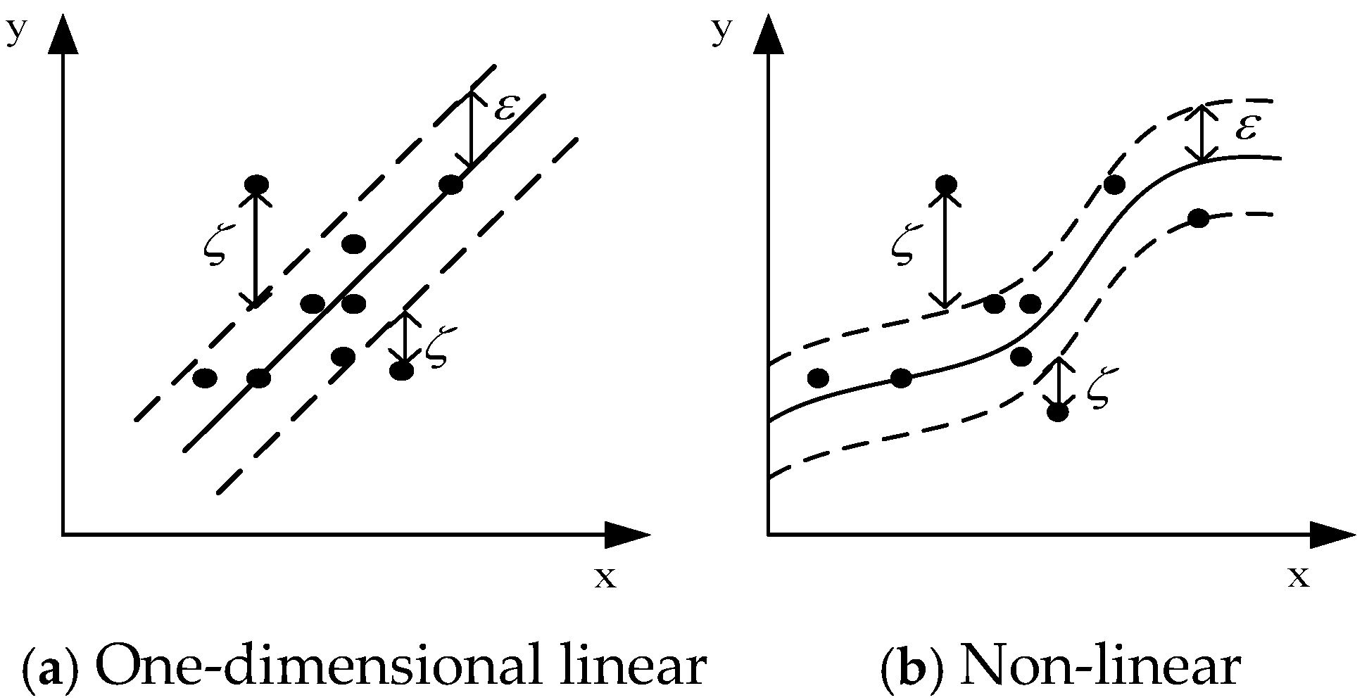
3.2. Support Vector Machine (SVM)

SVM is a learning method proposed by Vapnik and others in the 1990s based on statistical theory [36]. Nowadays, it finds wide applications in pattern recognition, regression analysis, feature extraction, and other fields. It is particularly suitable for predictions involving small sample sizes.

For regression SVM, an insensitive loss function is defined to ignore errors within a certain range around the actual values. Figure 1a,b, respectively, illustrate the $\epsilon$ insensitive zones of one-dimensional linear and nonlinear regression functions, and the $\xi$ variable represents the error cost at the training points.

Given sample data $\left\{x_i,y_i\right\}, i=1, 2, \dots , l, x_i\in R^n, y_i\in R$, $x_i$ and $y_i$, respectively, represent the sample inputs and outputs. The estimated regression function is found in the set of linear functions: $f(x)=b+w\cdot x$, $w, x\in R^n, b\in R$. To ensure a solution exists, slack variables $\xi$ and $\stackrel{\wedge }{\xi }$ are introduced. Then, it is transformed into solving the following function problem:

$$\min \phi (w)={\displaystyle \frac{1}{2}}{‖w‖}^2+G{\displaystyle \sum _{i=1}^l({\xi }_i+\stackrel{\wedge }{{\xi }_i})}$$

(8)

$$\mathit{subject}\mathit{to}\left\{\begin{array}{c}{y}_i-((w\cdot x_i)+b)\le \epsilon +{\xi }_i\\ \begin{array}{c}((w\cdot x_i)+b)-y_i\le \epsilon +\stackrel{\wedge }{{\xi }_i}\\ {\xi }_i,\stackrel{\wedge }{{\xi }_i}\ge 0 i=1, \dots , l\end{array}\end{array}\right.$$

(9)

where G (G > 0) is a specified constant. Establishing $Lagrange$ function, the optimization problem in its dual form is:

$$\begin{array}{l}L(w,b,{\xi }_i,\stackrel{\wedge }{{\xi }_i})={\displaystyle \frac{1}{2}}{‖w‖}^2+G{\displaystyle \sum _{i=1}^l({\xi }_i+\stackrel{\wedge }{{\xi }_i})}-{\displaystyle \sum _{i=1}^l{a}_i[\epsilon +{\xi }_i-y_i+((w\cdot x_i)+b)}]-\\ {\displaystyle \sum _{i=1}^l\stackrel{\wedge }{a_i}[\epsilon +\stackrel{\wedge }{{\xi }_i}+y_i-((w\cdot x_i)+b)}]-{\displaystyle \sum _{i=1}^l(n_i{\xi }_i+\stackrel{\wedge }{{\eta }_i}\stackrel{\wedge }{{\xi }_i})}\end{array}$$

(10)

where $w, b, {\xi }_i, \stackrel{\wedge }{{\xi }_i}$ represent the original variable, $a_i, {\stackrel{\wedge }{a}}_i, \stackrel{\wedge }{{\eta }_i}, {\eta }_i$ represent the dual variable, and both are greater than zero. Through calculation, we can finally obtain $w$ and the estimated function:

$$\left\{\begin{array}{c}w={\displaystyle \sum _{i=1}^l{x}_i(a_i-{\stackrel{\wedge }{a}}_i)}\hfill \\ f(x)={\displaystyle \sum _{i=1}^l(x_i,x)(a_i-{\stackrel{\wedge }{a}}_i)+b}\end{array}\right.$$

(11)

Introducing a kernel function $K(x,x^{\prime })$, the regression function becomes:

$$f(x)={\displaystyle \sum _{i=1}^{l}K(x_i,x)(a_i-{\stackrel{\wedge }{a}}_i)+b}$$

(12)

3.3. Optimization Algorithm

The initialization values of parameters in both the BPNN and SVM models are crucial, as they directly determine the prediction performance of the models. For the BPNN, selecting appropriate initial weights and thresholds is crucial. Optimization algorithms can be applied to find optimal values, thereby enhancing the performance of the neural network. For SVM, after selecting the RBF function as the kernel function based on the characteristics of the research object and literature studies [37,38,39,40], it is critical to set the penalty parameter (C) and the kernel function parameter (g) properly. Only with appropriate parameters can the transformed samples be effectively distributed in high-dimensional space. Since no single optimization method fits all scenarios, this study selects several optimization algorithms that have been widely validated as effective in other fields, including Particle Swarm Optimization (PSO), Genetic Algorithm (GA), and Grid Search Algorithm (GSA). These algorithms are used to optimize the parameters of both BPNN and SVM models, and the most suitable machine learning model is selected through comparison.

Genetic Algorithm (GA) is an evolutionary algorithm inspired by natural selection, initially proposed by Professor Holland. Key parameters include the number of generations, population size, crossover probability, and mutation probability.

The Particle Swarm Optimization (PSO) algorithm, inspired by bird foraging behavior, was proposed by Kennedy and Eberhart in 1995 as a swarm intelligence optimization technique. In PSO, each particle represents a potential solution in an N-dimensional search space and has two key attributes: position, which indicates the current solution, and velocity, which determines how the position is updated during the search process. The entire process iterates continuously until meeting the final condition.

The Grid Search Algorithm (GSA) is a simple and straightforward method for parameter optimization. In this study, it is primarily applied to optimize the parameters of the SVM. The essence of GSA lies in evaluating different parameter combinations in a grid format to identify the optimal one. However, when the number of parameters is large, GSA becomes computationally intensive and time-consuming, making it more suitable for problems with fewer variables.

3.4. Hyperparameter Settings

In the application of the BPNN, optimization algorithms can be used to assign optimized initial weights and thresholds, thereby improving its predictive performance. In the GA-BPNN experiments, based on previous studies and a controlled variable analysis [41,42], the population size was set to sizepop = 20, the number of generations to maxgen = 100, the crossover probability to pcross = 0.5, and the mutation probability to pmutation = 0.01. For the PSO-BPNN experiments, parameter settings were determined with reference to related literature and controlled variable analysis [43,44,45]. The PSO algorithm was configured with a swarm size of size = 20 and a maximum iterations number of Tmax = 100. The initial inertia weight was set to 0.9 and decreased linearly to 0.4. The cognitive and social learning factors were both set to C₁ = C₂ = 2.

In the application of SVM models, optimization algorithms enable an efficient search for near-optimal values of the penalty factor C and kernel parameter g within a short time. Based on comparative experiments, the SVM model adopted the Radial Basis Function (RBF) kernel. In the GA-SVM experiments, the parameter search ranges were set to C ∈ [0, 100] and g ∈ [0, 100]. For the PSO-SVM experiments, the search ranges were set to C ∈ [2⁻⁵, 100] and g ∈ [2⁻⁵, 100]. The parameter settings for GA and PSO followed those described earlier. In the GSA-SVM experiments [46,47], a step size of 0.5 was used for both the penalty parameter (cstep) and the kernel parameter (gstep). The initial search ranges for the parameters were set as C ∈ [2⁻⁸, 28] and g ∈ [2⁻⁸, 28], respectively.

4. Determination of Indicators and Data Processing

4.1. Determination and Assignment of Indicators

Before applying machine learning methods to cost estimation for office buildings, it is essential to establish a set of indicators. These indicators correspond to the engineering feature vectors, which serve as the input values for the model. Based on the literature review [13,24,26,32,33,48,49,50,51], the indicators are consolidated and analyzed statistically. Some are further optimized as needed. For example, indicators that appear only once are removed. Similar indicators with overlapping concepts, such as “Number of floors”, “Number of floors above ground”, and “Number of floors below ground”, are integrated or adjusted. As a result, the “Number of floors” indicator is deleted because it overlaps with the others.

After the above processing, the indicators are further organized and analyzed statistically. Use the expert scoring method for indicator selection, and delete redundant indicators that have little impact on cost estimation. Finally, experts from 6 construction units, 4 design units, and 5 construction units were selected. The concentration and dispersion of expert opinions were analyzed to screen the data. Based on expert opinions, the final selection of indicators was determined, and the specific indicator system for estimating the cost of office buildings is presented in

Table 1. Indicator system for estimating the cost of office buildings.

Serial Number	Indicator	Unit	Serial Number	Indicator	Unit
X1	Floor area	m2	X10	Base type	-
X2	Underground floor area	m2	X11	Number of elevators	set
X3	Structure type	-	X12	Internal decoration Level	-
X4	Height	m	X13	External decoration level	-
X5	Number of floors above ground	floor	X14	Installation completeness	-
X6	Number of floors below ground	floor	X15	Engineering cost index	-
X7	Average height above ground	m	X16	Steel price index	-
X8	Average height below ground	m	X17	Concrete price index	-
X9	Seismic grade	grade

.

Before training the model, it is necessary to quantify each indicator in the indicator system. For quantifiable indicators, the value can be directly obtained from the corresponding actual engineering data. For qualitative indicators, values are quantified from low to high according to cost. Qualitative indicators are assigned values from 1 to 5 based on their different properties, where a higher value indicates a higher corresponding price and a greater impact on the unit cost.

4.2. Data Collection

Based on the established cost estimation indicator system for office buildings, data collection for case indicators is conducted. Regional disparities in policy environment, geological conditions, and other fundamental factors are significant. However, within the same region, conditions tend to be more similar, which benefits model training [52]. Therefore, this paper selects a province in China as the study area. To ensure convenience in data acquisition, Hubei Province was chosen as the case study region. Given that the unit cost indicator is more representative than the overall project cost, and unit cost data are more readily available during case collection, this paper adopts the unit construction cost as the final predicted value for the model.

Data on newly completed office buildings in Hubei Province over the past six years were collected and organized. After removing data with severe missing information, 115 valid cases were initially obtained. Statistical analysis revealed that only 2 cases involved steel structures, 2 involved frame-tube structures, and 1 involved masonry structures. These three types of structural systems have a significant impact on the overall cost. To avoid potential biases in the predictive performance due to insufficient training data, these 5 cases were excluded. Consequently, a total of 110 valid data were obtained. It is important to note that the construction unit cost used in this study refers to the final settlement price at project completion. Decision-stage obtainable indicator data serve as the model’s input vectors, while the final settlement price serves as the output vector. For missing data, we employed a constant value imputation method.

4.3. Dimensionality Reduction of Indicators

Estimating office building costs involves numerous indicators, and even after refinement, the final indicator system still contains a large number of variables. To avoid overfitting caused by extracting too many features and to improve the prediction accuracy of the model, it is necessary to conduct dimensionality reduction on the indicators. We select Principal Component Analysis (PCA) and Grey Relational Analysis (GRA), two widely adopted methods in machine learning, to perform this task. GRA quantitatively evaluates the correlation between influencing factors, allowing us to better understand how each factor relates to engineering cost within the indicator system. However, some information may be lost during dimensionality reduction. PCA, in contrast, seeks to reduce the number of indicators while preserving as much original information as possible, though it requires greater computational effort. Both methods have their respective advantages, so we choose to employ both approaches for dimensionality reduction. We will then compare the predictive results of the models to select the optimal dimensionality reduction method.

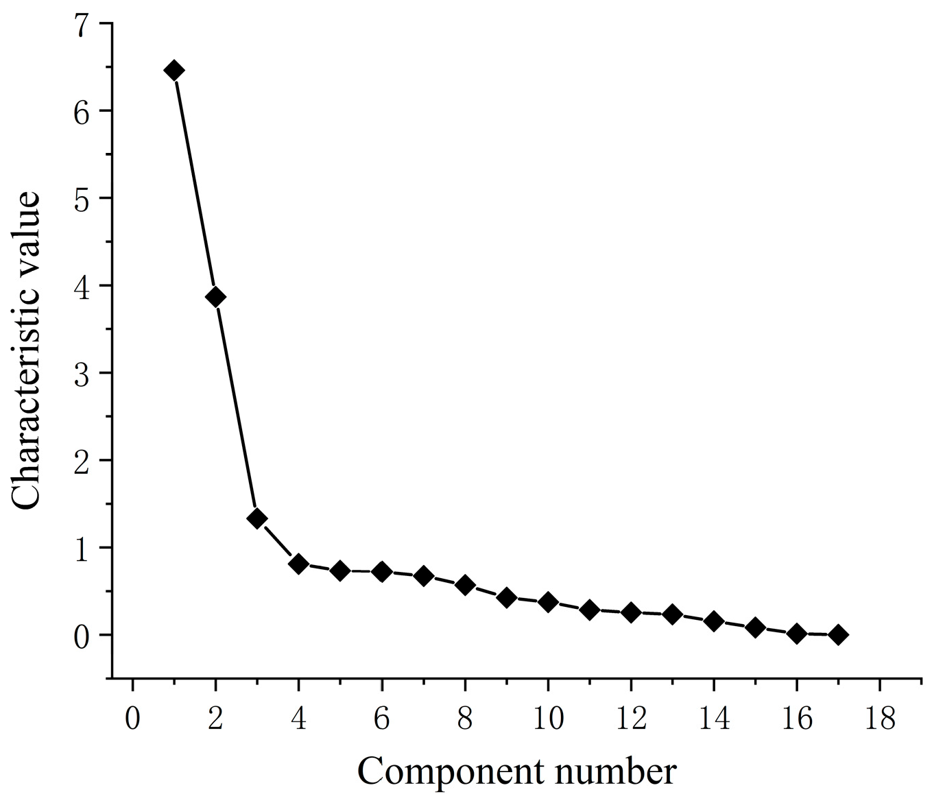
4.3.1. PCA for Dimensionality Reduction

We use the heatmap function to visualize the correlation coefficients between feature variables, as shown in Figure 2. On the right side of the figure is the color scale, where different colors represent varying degrees of correlation between variables. The closer the color is to purple, the stronger the correlation. As the heatmap illustrates, most indicators exhibit varying degrees of intercorrelation. To improve model performance and eliminate multicollinearity, we apply Principal Component Analysis (PCA) for dimensionality reduction.

Observations reveal that the unit construction cost exhibits correlation coefficients greater than 0.6 with five feature variables: external decoration level, installation completeness, average height above ground, steel price index, and concrete price index. These correlations are relatively significant. The dependent variable shows correlation coefficients ranging from 0.4 to 0.6 with four feature variables: internal decoration level, base type, average height below ground, and engineering cost index. Correlation coefficients can partially reflect the importance of these indicators. Therefore, the nine indicators mentioned above have a significant impact on the unit cost.

Utilizing IBM SPSS Statistics (version 24.0), principal component analysis was conducted on the dataset. The KMO measure of sampling adequacy was 0.792, surpassing the threshold of 0.7, and Bartlett’s test of sphericity yielded a p-value below 0.001. These results confirm that the input variables are significantly correlated, indicating that the dataset is suitable for subsequent factor analysis. To retain as much information as possible, we extracted the first seven principal components, which together explain 85.903% of the total variance—capturing the majority of the dataset’s information. As illustrated in the scree plot for office building cost estimation (Figure 3), the first seven factors account for most of the variance, indicating that they retain most of the original information.

We obtained the factor score coefficient matrix from the SPSS analysis. Based on this matrix, we derived expressions for each of the seven common factors, denoted as $F_1$ through $F_7$. For instance, the expression for the first common factor ($F_1$) is as follows:

$$\begin{array}{l}{F}_1=0.793x_1+0.772x_2+0.611x_3+0.816x_4+0.796x_5+0.840x_6+0.374x_7\\ +0.733x_8+0.197x_9+0.616x_{10}+0.837x_{11}+0.307x_{12}+0.350x_{13}+0.458x_{14}+\\ 0.300x_{15}+0.559x_{16}+0.483x_{17}\end{array}$$

Following the same procedure, we derive expressions for all seven factors. Then, by substituting these expressions into the Z-score standardized data, we calculate the input data for the principal component analysis.

4.3.2. GRA for Dimensionality Reduction

GRA evaluates the similarity of the geometric shapes of sequence curves to assess the closeness of relationships between factors, while correlation analysis examines the degree of linear correlation between variables through data analysis. These two methods have certain differences. In this study, a resolution coefficient of 0.2 was chosen. The final grey relational coefficients are presented in

Table 2. Grey relational coefficient.

Serial Number	Indicator	Correlation Coefficient	Serial Number	Indicator	Correlation Coefficient
X17	Concrete price index	0.890	X3	Structure type	0.836
X14	Installation completeness	0.883	X8	Average height below ground	0.661
X16	Steel price index	0.881	X4	Height	0.656
X7	Average height above ground	0.862	X5	Number of floors above ground	0.653
X12	Internal decoration Level	0.855	X6	Number of floors below ground	0.629
X15	Engineering cost index	0.855	X11	Number of elevators	0.606
X10	Base type	0.850	X1	Floor area	0.600
X9	Seismic grade	0.847	X2	Underground floor area	0.561
X13	External decoration level	0.838

. Considering the number of indicators, the results of correlation analysis, and the discontinuity of grey relational coefficients, we set a correlation threshold of 0.80. Accordingly, the top ten indicators with grey relational coefficients exceeding 0.80 were selected as input vectors for subsequent model prediction.

5. Estimation Model Prediction and Comparison

5.1. Estimation Model Prediction

Based on MATLAB (R2018b), BPNN, GA-BPNN, and PSO-BPNN prediction models were established separately. Multiple controlled variable experiments were conducted to optimize the structural and functional parameters of each model. To ensure accurate evaluation, three regression metrics were selected: mean squared error ($MSE$), squared correlation coefficient ($R^2$), and mean absolute percentage error ($MAPE$), with the corresponding formulas shown below.

$$MSE={\displaystyle \frac{1}{n}}{\displaystyle \sum _{i=1}^n{(y_i-\stackrel{\wedge }{y_i})}^2}$$

(13)

$$R^2={\displaystyle \frac{{(n{\displaystyle \sum _{i=1}^n\stackrel{\wedge }{y_i}}{y}_i-{\displaystyle \sum _{i=1}^n\stackrel{\wedge }{y_i}}{\displaystyle \sum _{i=1}^n{y}_i})}^2}{(n{\displaystyle \sum _{i=1}^n{(\stackrel{\wedge }{y_i})}^2}-{({\displaystyle \sum _{i=1}^n\stackrel{\wedge }{y_i}})}^2)(n{\displaystyle \sum _{i=1}^n{y_i}^2}-{({\displaystyle \sum _{i=1}^n{y}_i})}^2)}}$$

(14)

$$MAPE={\displaystyle \frac{1}{n}}{\displaystyle \sum _{i=1}^n\left|\frac{y_i-\stackrel{\wedge }{y_i}}{y_i}\right|}$$

(15)

where ${\widehat{y}}_i$ is the predicted value, $y_i$ is the true value, and n is the number of predicted samples. To minimize overfitting in the BPNN and improve prediction accuracy, the data is normalized using the mapminmax function, which eliminates differences in the magnitude of the sample data. In this study, $MSE$ and $R^2$ are calculated using the normalized data, while $MAPE$ is calculated based on the actual data.

To evaluate and select the cost estimation models, this study adopts the holdout method. The predictive results obtained from a single holdout are often not reliable and stable enough. Therefore, it is common practice to perform multiple random partitions and repeated experiments to assess the models, and then take the average as the evaluation result [53]. In this study, the randperm function is used to randomly generate training and testing samples from the 106 samples. Specifically, 90 randomly generated samples are assigned to the training set, while the remaining 16 samples are allocated to the testing set. Each model is subjected to 200 experiments with randomly generated 200 sets of distinct training and testing datasets. After conducting experiments separately for each model, the average values of the evaluation metrics are calculated and compared for analysis.

5.1.1. BPNN Prediction Model

The number of hidden layers, the number of nodes in each hidden layer, and the choice of transfer functions significantly influence the prediction performance of BPNN models. Therefore, experiments were conducted to optimize these parameters and enhance the model’s predictive accuracy. To determine the optimal number of hidden layers, this study compared single-layer and double-layer architectures, considering the relatively simple structure of the sample data [54]. The optimal number of hidden nodes was identified through trial-and-error within a predefined range. For the transfer functions, three commonly used functions—purelin, tansig, and logsig—were tested in various combinations to determine the most effective configuration.

Through controlled variable experiments, the optimal BPNN structure for predicting the original dataset was identified. The best performance was obtained with a single hidden layer containing eight nodes, using the logsig activation function in the hidden layer and purelin in the output layer. Under this configuration, the BPNN achieved average results across 200 simulation runs of MSE = 0.058, R² = 0.846, and MAPE = 7.73%. Figure 4 presents both the line chart and scatter plot of the prediction results from one representative experimental run.

After performing principal component analysis (PCA) on the dataset, the original 17 input indicators were reduced to 7 principal components, necessitating corresponding adjustments to the BPNN structure. Based on a series of controlled experiments, the optimal PCA-BPNN configuration was identified as a single hidden layer with four nodes, using tansig as the activation function for both the hidden and output layers.

Similarly, following the application of grey relational analysis (GRA), ten indicators with the highest grey relational coefficients were selected from the original 17 variables as model inputs. The optimal structure for the GRA-BPNN model was determined to consist of a single hidden layer with five nodes, employing a logsig activation function in the hidden layer and purelin in the output layer.

GA and PSO were used to optimize the initial weights and thresholds of the BPNN, thereby enhancing its predictive performance. During the simulations of the GA-BPNN and PSO-BPNN models, the network structures and activation functions were kept consistent. Each model was subjected to 200 experimental runs, and the average values of the prediction evaluation metrics were calculated to assess overall model performance.

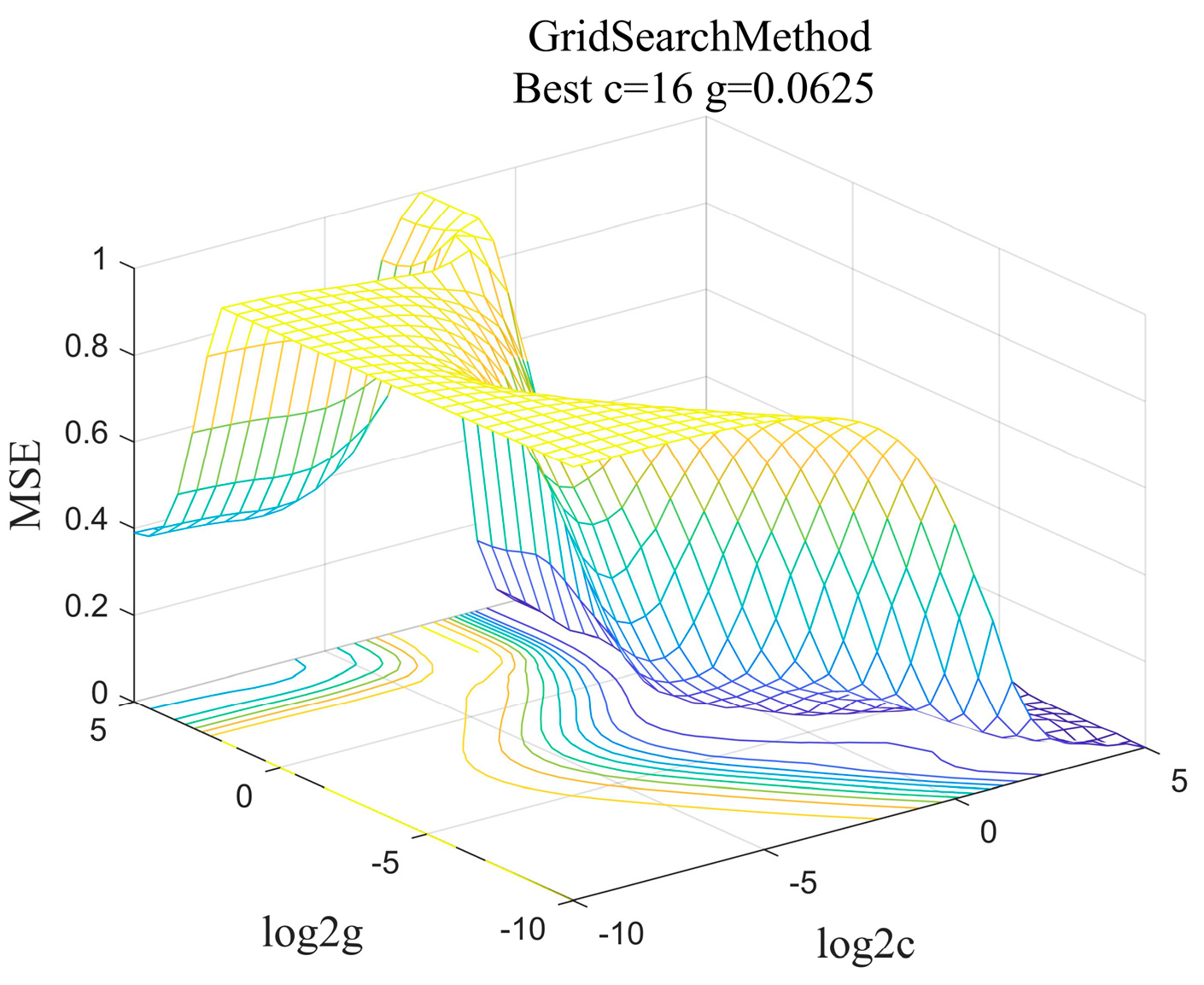
5.1.2. SVM Prediction Model

GSA-SVM, GA-SVM, and PSO-SVM prediction models were constructed. To minimize the occurrence of overfitting in SVM, the models needed to utilize the mapminmax function to normalize the data during application.

During the optimization of the SVM model using grid search, a fitness curve plot can be obtained, representing the parameter selection results based on cross-validation mean squared error. This plot provides a visual representation of the optimization process of the grid search method. Figure 5 presents a three-dimensional plot of one experimental run, showing the parameter selection results, where the optimal parameters were determined as C = 16 and g = 0.0625.

5.2. Comparison Analysis of Prediction Results

We observed that the three error evaluation metrics show consistent trends during optimization. Since R² and MAPE offer clearer comparisons, we used their average as the evaluation criterion.

Table 3. Comparison of predictive performance among six model types.

Prediction Model	Raw Data		PCA		GRA
	R2	MAPE	R2	MAPE	R2	MAPE
BPNN	0.846	7.73%	0.855	7.35%	0.836	7.67%
GA-BPNN	0.874	6.65%	0.899	6.19%	0.877	6.57%
PSO-BPNN	0.853	7.71%	0.861	7.23%	0.833	7.63%
GA-SVM	0.885	6.75%	0.888	6.42%	0.867	6.99%
PSO-SVM	0.882	6.57%	0.892	6.29%	0.847	6.82%
GSA-SVM	0.902	5.94%	0.927	5.52%	0.893	6.23%

presents the specific results.

A comprehensive analysis of Table 3 yields the following conclusions:

(1)

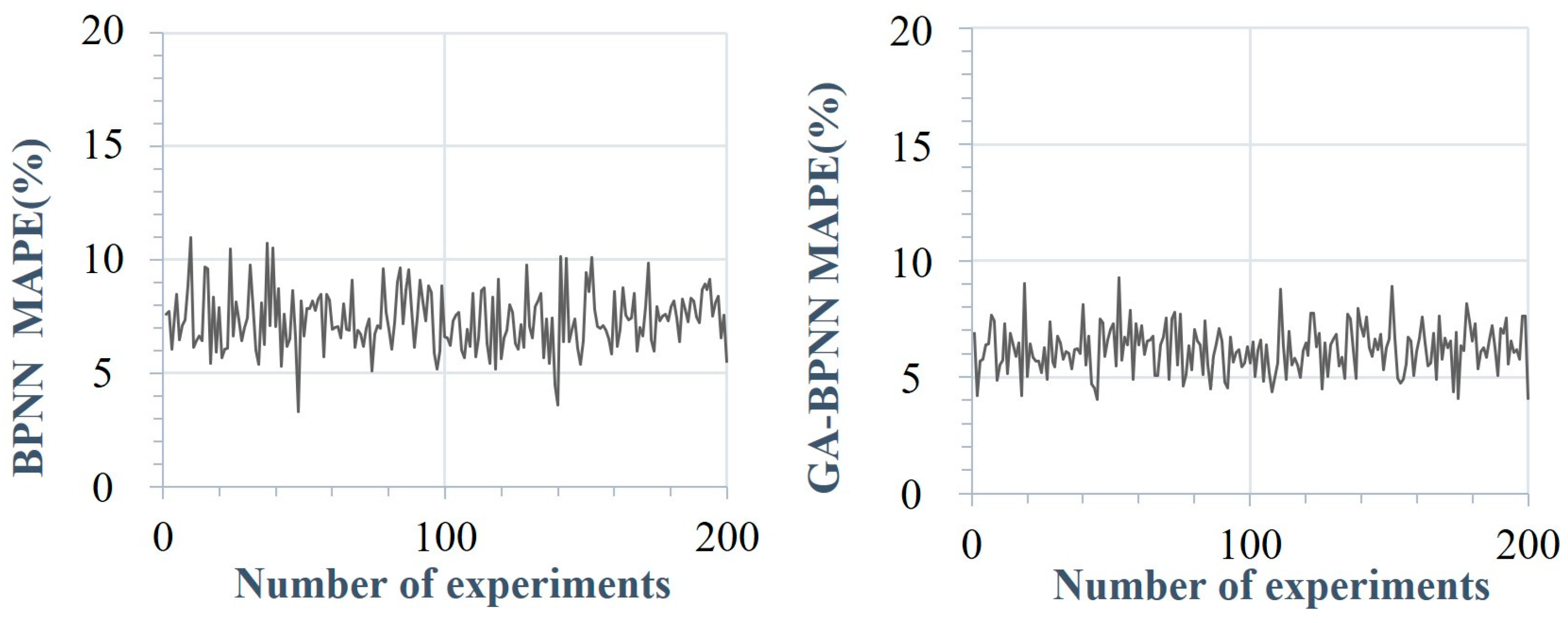
After structural optimization and parameter tuning, all six prediction models—BPNN, GA-BPNN, PSO-BPNN, GA-SVM, PSO-SVM, and GSA-SVM—achieved strong predictive performance. The original BPNN also performed well in this study. All models maintained MAPE below 8% and mean squared correlation coefficients above 0.8.

(2)

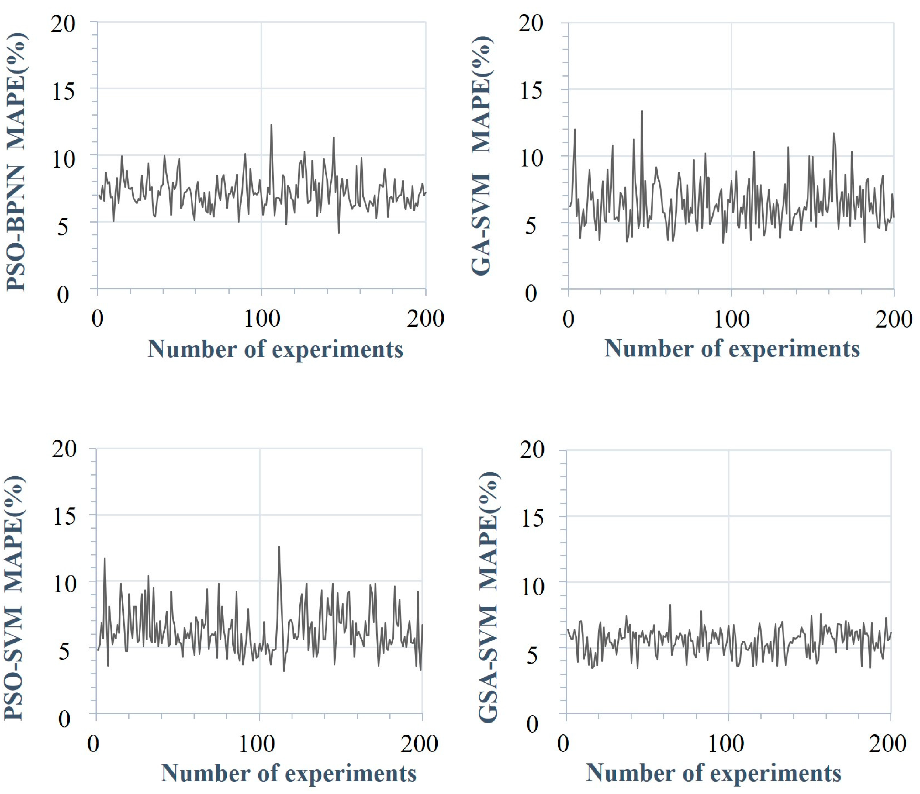
In terms of algorithm optimization, GA and PSO optimization significantly improved the predictive performance of the BPNN model, demonstrating the value of algorithm optimization in machine learning. The optimization effects varied across models: GA outperformed PSO in BPNN, while PSO showed better results than GA in SVM. The optimal machine learning model varies for different research problems. When selecting optimization algorithms, one should consider both data characteristics and model structure. Comparative analysis may help identify the most suitable optimization approach.

(3)

In terms of dimensionality reduction methods, PCA dimensionality reduction improved the predictive performance of all six models. However, GRA dimensionality reduction had mixed effects. It slightly improved performance in BPNN, GA-BPNN, and PSO-BPNN, but worsened the performance in GA-SVM, PSO-SVM, and GSA-SVM models. This may be due to GRA’s loss of some information during dimensionality reduction, which certain models are sensitive to. Therefore, selecting the right dimensionality reduction method is crucial in machine learning. Conducting comparative studies can help determine the best approach.

(4)

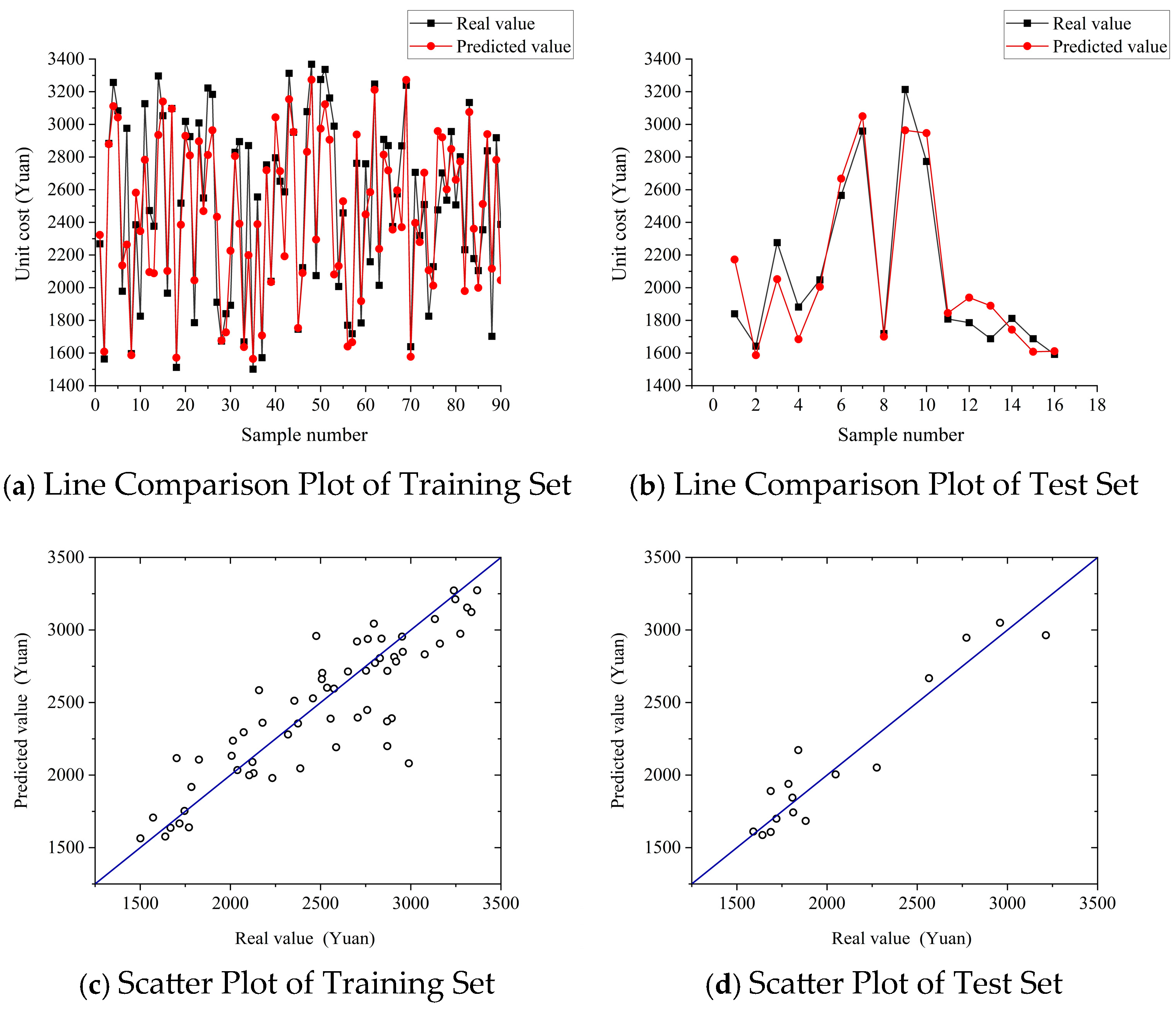
In terms of model selection, the PCA-GSA-SVM model exhibits the best predictive performance among all established models, with an R² of 0.927 and MAPE of 5.52%. The predictive accuracy has reached a relatively ideal level.

5.3. Prediction Model Comprehensive Comparison and Selection

Based on a review of relevant literature and practical applications, three evaluation criteria were selected: accuracy, stability, and computation time. Since the computation times are generally similar among models of the same type, and models incorporating PCA tend to yield superior performance, six PCA-based models were selected for horizontal comparative analysis.

5.3.1. Accuracy Comparison

Given that R² and MAPE provide essentially the same information and MAPE exhibits more pronounced fluctuations, we conducted a stability comparison analysis on MAPE indicators. Figure 6 illustrates scatter plots of the indicators from 200 experiments for each model under PCA. Upon comparison, the predictive accuracy of each model ranks as follows: GSA-SVM > GA-BPNN > PSO-SVM > GA-SVM > PSO-BPNN > BPNN. The GSA-SVM model has the lowest overall MAPE, with relatively few occurrences of outliers.

The GSA-SVM model delivers the most accurate predictions in this study. GSA, as a basic parameter optimization algorithm for SVM, is simple, easy to understand, and provides good prediction results. However, GSA is not ideal for complex, large-scale data samples. As the search range increases, the prediction time cost of GSA rises significantly. Given the limited data in this study, the GSA-SVM model is well suited to this context. For more complex problems, models optimized by heuristic algorithms can also achieve good prediction accuracy. In the case of office building cost estimation, if the GSA-SVM model does not perform well, the GA-BPNN model can serve as an alternative for prediction.

5.3.2. Stability Comparison

The BPNN, SVM, and their respective optimization algorithms all have a certain inherent instability. In this study, the training and testing sets were randomly selected for each experiment, causing fluctuations in the model’s predictive evaluation indicators.

The stability comparison will be approached from two perspectives: Firstly, the fluctuation of MAPE in the 200 experiments’ testing sets, as shown in Figure 5. Secondly, the range of prediction error rates for 16 selected testing sets.

(1) Stability of the MAPE

We obtained the maximum and minimum values of the MAPE among the 200 experiments for each model under PCA, and calculated the range of error fluctuations. The results are presented in

Table 4. The fluctuation range of MAPE.

Prediction Model	Range of MAPE Fluctuations
BPNN	[3.32%, 10.98%]
GA-BPNN	[4.02%, 9.28%]
PSO-BPNN	[4.16%, 12.27%]
GA-SVM	[3.47%, 13.38%]
PSO-SVM	[3.19%, 12.63%]
GSA-SVM	[3.42%, 8.26%]

.

By observing Figure 6 and Table 4, the following conclusions can be drawn: The prediction error range of the PCA-GSA-SVM model is the smallest, [3.42%, 8.26%], with an absolute difference of 4.84%. The PCA-GA-BP model follows closely, with an absolute difference of 5.26%. From Figure 6, it is evident that the fluctuations in MAPE of the PCA-GSA-SVM and PCA-GA-BP models are relatively stable, with errors maintained at a low level. Overall, all models exhibit good stability after tuning, with the MAPE of each model in every experiment kept within 14.00%.

(2) Test set error stability

Given that the PCA-GSA-SVM model performs well in both prediction accuracy and stability, we further examine the stability of its specific test set cases. We analyze the detailed prediction data of 16 test sets when the MAPE is at its lowest and highest for the GSA-SVM model, as shown in

Table 5. Prediction errors for PCA-GSA-SVM Model on test sets.

Sample Number	Prediction Error Mean at Highest (MAPE = 8.26%)			Prediction Error Mean at Lowest (MAPE = 3.42%)
	Real Value	Predicted Value	Error Rate	Real Value	Predicted Value	Error Rate
1	3274.99	3121.76	−4.68%	3133.99	3147.48	0.43%
2	1719.34	1928.21	12.15%	2761.87	2814.62	1.91%
3	2555.61	2587.22	1.24%	3053.02	3059.97	0.23%
4	2374.80	2145.73	−9.65%	1745.66	1599.38	−8.38%
5	1978.45	2012.05	1.70%	2702.58	2521.83	−6.69%
6	2549.52	2327.57	−8.71%	2104.47	2157.80	2.53%
7	3313.10	3280.04	−1.00%	2752.24	2717.08	−1.28%
8	2318.60	2745.94	18.43%	1563.76	1700.06	8.72%
9	2457.91	2541.17	3.39%	1718.03	1673.89	−2.57%
10	1786.14	1560.63	−12.63%	3106.52	3239.94	4.29%
11	1840.65	1926.69	4.67%	2275.81	2332.46	2.49%
12	2507.18	2672.30	6.59%	1812.13	1830.36	1.01%
13	1642.32	1796.69	9.40%	1501.20	1435.32	−4.39%
14	3296.30	3041.86	−7.72%	2517.75	2504.51	−0.53%
15	2473.80	2931.32	18.49%	2989.15	3127.56	4.63%
16	1638.89	1447.54	−11.68%	2509.37	2626.13	4.65%

. For a more intuitive analysis of the stability of model predictions, we have plotted line comparison and scatter plots based on the data from Table 5, as shown in Figure 7.

As shown in Table 5, the PCA-GSA-SVM model achieves the lowest MAPE of 3.42%. Across the 16 test sets, the prediction errors range from −8.38% to 8.72%, with all predicted values falling within a 10.00% margin of error. The maximum MAPE observed is 8.26%. Throughout all test sets, prediction error rates remain below 20.00%, and most cases exhibit error rates under 10.00%.

Figure 7 visually demonstrates that the predictive performance of the PCA-GSA-SVM model has reached a satisfactory level. In both (a) and (b) plots, it is evident that the actual values closely align with the predicted values, indicating a high degree of concordance and a well-fitted model. In contrast, in plots (c) and (d), it is noticeable that the scatter points are concentrated around the center line. Here, the blue line represents the 10% error line, while the red line represents the 20% error line. When the MAPE is at its lowest, all scatter points fall within the 10% error range. Even at the highest MAPE, most points remain within 10%, and all are within 20%. In conclusion, the PCA-GSA-SVM model largely meets the error requirements during the feasibility study phase of the decision-making process. It fully meets the error requirements during the investment opportunity research phase and the preliminary feasibility study phase, thus holding practical significance.

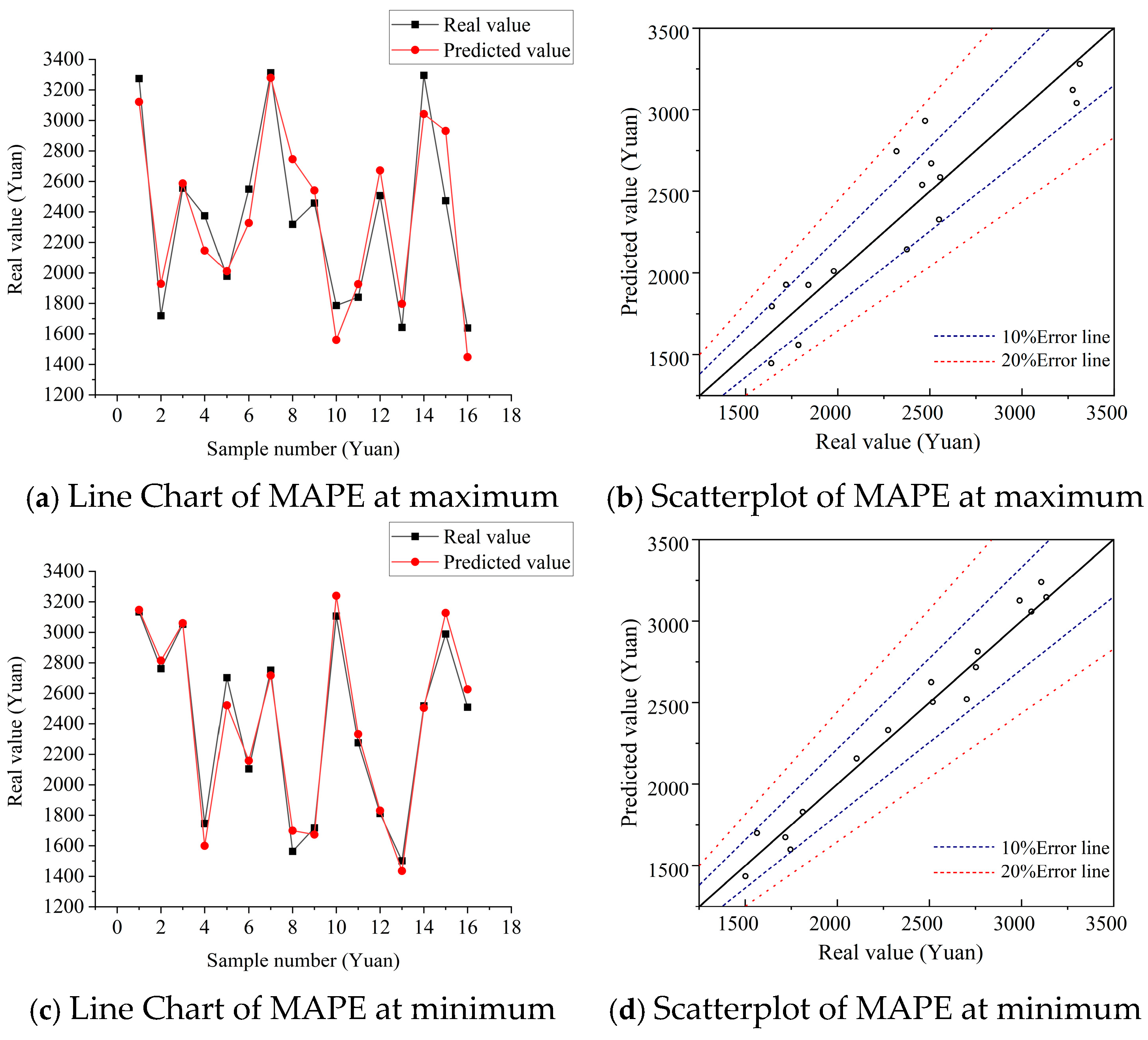
5.3.3. Comparison of Fixed Test Set Results

We used the randperm function to randomly generate 90 training sets and 16 test sets from 106 samples. These sets were kept fixed for the analysis. We then applied the six PCA-based models to predict outcomes for this fixed set. To visualize the results, we plotted the predictions from the six models as a scatter plot, as shown in Figure 8.

Based on the analysis of Figure 8, the following observations were made: (1) The PSO-BPNN and BPNN models have more scatter points exceeding the 10% error line. Additionally, their scatter points are less concentrated around the central line, indicating relatively poorer overall prediction performance. (2) The PSO-SVM and GA-SVM models have most scatter points within the 10% error line, with only a few outliers. The points are relatively concentrated around the center line, indicating a generally good predictive performance. However, the stability of these models is somewhat lacking. (3) Both the GA-BPNN and GSA-SVM models exhibit the highest concentration of scatter points near the center line. However, the GA-BPNN model has one scatter point slightly exceeding the 10% error line, whereas all scatter points for the GSA-SVM model remain within the 10% error line. In conclusion, the PCA-GSA-SVM model shows the best prediction accuracy and stability, consistent with earlier comparisons.

5.3.4. Time Comparison

Each optimization algorithm includes an iterative search process based on machine learning. This process inevitably increases both training and prediction time. The effect is more pronounced when parameters such as the number of evolutionary generations and population size are set to high values. Under these conditions, the runtime of each model is significantly prolonged. While maintaining prediction accuracy and stability, it is also essential to keep the computational time within a reasonable range to ensure overall predictive efficiency. We recorded the execution time for each model using the ‘tic’ and ‘toc’ functions. The results are presented in

Table 6. Time comparative analysis.

	BPNN	GA-BPNN	PSO-BPNN	GA-SVM	PSO-SVM	GSA-SVM
Single Prediction Time	2.036 s	114.756 s	154.427 s	2.072 s	3.331 s	16.861 s

.

Due to the limited size of the training and prediction datasets in this study, the execution times for all models are relatively short. Among them, the BPNN model is the fastest, requiring only 2.036 s. The GA-SVM and PSO-SVM models follow closely, each completing a prediction in under 4 s. The GSA-SVM model takes 16.861 s, which is longer than the previous three but still within a reasonable and acceptable range. In contrast, the GA-BPNN and PSO-BPNN models exhibit the longest runtimes. Their execution times also tend to increase as the number of evolutionary generations and other parameters grow. The results suggest that applying optimization algorithms to BPNN significantly increases computational time. In comparison, optimization applied to SVM results in much shorter runtimes. This difference is mainly due to the larger number of search iteration nodes in BPNN and the inherent complexity of the model itself, which amplifies the time cost when combined with optimization techniques.

In summary, this study identifies the PCA-GSA-SVM model as the relatively optimal choice for office building cost estimation, considering its accuracy, stability, and computational efficiency. The model holds both theoretical and practical value for supporting decision-making in the early stages of office building projects. However, in real-world applications involving large volumes of cost data, the PCA-GSA-SVM model may require longer processing time. As a result, it is best suited for scenarios where accuracy is prioritized over speed—such as in most current project investment evaluations. For projects with strict time constraints, alternative models like BPNN or GA-SVM may be more appropriate, as they offer shorter processing times, albeit with slightly lower accuracy. Ultimately, model selection should be based on specific prediction requirements. Trade-offs among accuracy, stability, and computation time, as observed in this study, must be carefully considered to ensure appropriate model application.

6. Conclusions and Prospect

6.1. Conclusions

This study is based on machine learning and establishes cost estimation models using SVM and BPNN. It employs PSO, GA, and GSA to optimize the models, and compares and analyzes the prediction results of each model. The main conclusions of the article are as follows:

(1)

We constructed a cost estimation indicator system for office buildings and identified key influencing factors for unit costs. Through literature analysis, questionnaire surveys, and other methods, 17 cost estimation indices for office buildings were ultimately identified.

(2)

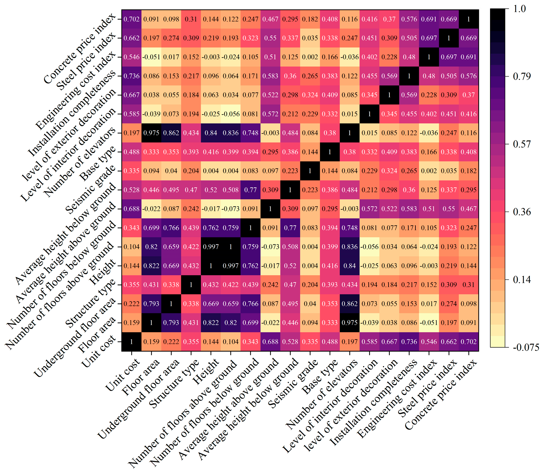
Through comprehensive analysis of the relevant coefficients and the gray correlation coefficients, it was found that the seven key influencing factors of the unit cost of office building construction are: internal decoration level, external decoration level, installation completeness, average height above ground, engineering cost index, steel price index, and concrete price index.

(3)

The utilization of PCA and optimization algorithms enhanced the predictive performance of the construction cost estimation model. When selecting data dimensionality reduction methods in machine learning, caution is required. In the field of construction cost estimation, PCA dimensionality reduction could be prioritized.

(4)

An optimized office building cost estimation model based on machine learning was identified in this study. The PCA-GSA-SVM predictive model yielded an average mean squared error of 0.024, a squared correlation coefficient of 0.927, and an average percentage error of 5.52% in experimental trials. Compared to traditional engineering cost estimation methods, this model demonstrates faster speed, higher accuracy, and stronger stability, addressing the limitations of conventional approaches. As a result, the model proposed in this paper provides significant theoretical and practical value for cost estimation during the decision-making stage of office building projects and can serve as a useful reference for other types of buildings as well.

6.2. Limitations and Further Studies

For machine learning models to make accurate and stable predictions, they require a vast amount of data to establish training patterns. Due to limitations in personal capacity, this study may have collected slightly insufficient cases. Furthermore, all data in this study were sourced from Hubei Province, and there is a lack of research assessing its applicability in other provinces or regions. In future research, we plan to enhance the variety and quantity of training samples by incorporating data from other provinces and international contexts. This will help improve the model’s generalizability, accuracy, and robustness.

References

1. Jin, H.Y.; Shen, L.Y.; Wang, Z. Mapping the Influence of Project Management on Project Cost. Ksce. J. Civ. Eng. 2018, 22, 3183–3195. [Google Scholar] [CrossRef]
2. Giel, B.K.; Issa, R.R.A. Return on Investment Analysis of Using Building Information Modeling in Construction. J. Comput. Civil. Eng. 2013, 27, 511–521. [Google Scholar] [CrossRef]
3. Yan, X.L.; Zhou, Y.X.; Li, T.; Zhu, F.F. What Drives the Intelligent Construction Development in China? Buildings 2022, 12, 1250. [Google Scholar] [CrossRef]
4. Zhao, J.Y.; Cao, Y.Z.; Xiang, Y.Z. Pose estimation method for construction machine based on improved AlphaPose model. Eng. Constr. Archit. Manag. 2024, 31, 976–996. [Google Scholar] [CrossRef]
5. Li, Z.J.; Peng, S.H.; Cai, W.G.; Cao, S.P.; Wang, X.; Li, R.; Ma, X.R. Impacts of Building Microenvironment on Energy Consumption in Office Buildings: Empirical Evidence from the Government Office Buildings in Guangdong Province, China. Buildings 2023, 13, 481. [Google Scholar] [CrossRef]
6. Jiang, Y.Z.; Guo, S.; Xia, J.; Wei, Q.; Zheng, W.; Zhang, Y.; Yin, S.; Fang, H.; Deng, J. 2020 Annual Report on China Building Energy Efficiency; China Architecture & Building Press: Beijing, China, 2020. [Google Scholar]
7. Zuo, J.; Xia, B.; Chen, Q.; Pullen, S.; Skitmore, M. Green building rating for office buildings–Lessons learned. J. Green. Build. 2016, 11, 131–146. [Google Scholar] [CrossRef]
8. Kouskoulas, V.; Abutouq, G. An influence matrix for project expediting. Eur. J. Oper. Res. 1989, 43, 284–291. [Google Scholar] [CrossRef]
9. Wall, D.M. Distributions and correlations in Monte Carlo simulation. Constr. Manag. Econ. 1997, 15, 241–258. [Google Scholar] [CrossRef]
10. Wei, L. Design of Sustainable Construction Cost Estimation System Based on Grey Theory—BP Model. J. Inf. Knowl. Manag. 2024, 23, 2450011. [Google Scholar] [CrossRef]
11. Hwang, S. Time series models for forecasting construction costs using time series indexes. J. Constr. Eng. Manag. 2011, 137, 656–662. [Google Scholar] [CrossRef]
12. Zhao, L.; Mbachu, J.; Zhang, H. Forecasting residential building costs in New Zealand using a univariate approach. Int. J. Eng. Bus. Manag. 2019, 11, 1847979019880061. [Google Scholar] [CrossRef]
13. Alshamrani, O.S. Initial cost forecasting model of mid-rise green office buildings. J. Asian Archit. Build. Eng. 2020, 19, 613–625. [Google Scholar] [CrossRef]
14. Dobrucali, E.; Demir, I.H. A simple formulation for early-stage cost estimation of building construction projects. Gradevinar 2021, 73, 819–832. [Google Scholar] [CrossRef]
15. Kasmire, J.; Zhao, A.R. Discovering the Arrow of Time in Machine Learning. Information 2021, 12, 439. [Google Scholar] [CrossRef]
16. Gurmu, A.; Miri, M.P. Machine learning regression for estimating the cost range of building projects. Constr. Innov. 2025, 25, 577–593. [Google Scholar] [CrossRef]
17. Pham, T.Q.D.; Le-Hong, T.; Tran, X.V. Efficient estimation and optimization of building costs using machine learning. Int. J. Constr. Manag. 2023, 23, 909–921. [Google Scholar] [CrossRef]
18. Devyatkin, D.; Otmakhova, Y. Methods for Mid-Term Forecasting of Crop Export and Production. Appl. Sci. 2021, 11, 10973. [Google Scholar] [CrossRef]
19. Szoplik, J. Forecasting of natural gas consumption with artificial neural networks. Energy 2015, 85, 208–220. [Google Scholar] [CrossRef]
20. Xiong, Y.; Ming, Y.; Liao, X.H.; Xiong, C.Y.; Wen, W.; Xiong, Z.W.; Li, L.; Sun, L.P.; Zhou, Q.P.; Zou, Y.X.; et al. Cost prediction on fabricated substation considering support vector machine via optimized quantum particle swarm optimization. Therm. Sci. 2020, 24, 2773–2780. [Google Scholar] [CrossRef]
21. Zhang, S.H.; Wang, C.; Liao, P.; Xiao, L.; Fu, T.L. Wind speed forecasting based on model selection, fuzzy cluster, and multi-objective algorithm and wind energy simulation by Betz’s theory. Expert. Syst. Appl. 2022, 193, 116509. [Google Scholar] [CrossRef]
22. Chen, C.C.; Zhang, Q.; Kashani, M.H.; Jun, C.; Bateni, S.M.; Band, S.S.; Dash, S.S.; Chau, K.W. Forecast of rainfall distribution based on fixed sliding window long short-term memory. Eng. Appl. Comp. Fluid. 2022, 16, 248–261. [Google Scholar] [CrossRef]
23. Stulajter, F. Predictions in time series using multivariate regression models. J. Time. Ser. Anal. 2001, 22, 365–373. [Google Scholar] [CrossRef]
24. Dursun, O.; Stoy, C. Conceptual Estimation of Construction Costs Using the Multistep Ahead Approach. J. Constr. Eng. Manag. 2016, 142, 04016038. [Google Scholar] [CrossRef]
25. Leśniak, A.; Górka, M. Pre-design cost modeling of facade systems using the GAM method. Arch. Civ. Eng. 2021, 67, 123–138. [Google Scholar] [CrossRef]
26. Jin, R.; Cho, K.; Hyun, C.; Son, M. MRA-based revised CBR model for cost prediction in the early stage of construction projects. Expert. Syst. Appl. 2012, 39, 5214–5222. [Google Scholar] [CrossRef]
27. Juszczyk, M.; Lesniak, A. Modelling Construction Site Cost Index Based on Neural Network Ensembles. Symmetry 2019, 11, 411. [Google Scholar] [CrossRef]
28. Dong, J.C.; Chen, Y.; Guan, G. Cost Index Predictions for Construction Engineering Based on LSTM Neural Networks. Adv. Civ. Eng. 2020, 2020, 1–14. [Google Scholar] [CrossRef]
29. Pessoa, A.; Sousa, G.; Furtado Maués, L.M.; Campos Alvarenga, F.; Santos, D.d.G. Cost Forecasting of Public Construction Projects Using Multilayer Perceptron Artificial Neural Networks: A Case Study. Ing. E Investig. 2021, 41, 3. [Google Scholar] [CrossRef]
30. Sitthikankun, S.; Rinchumphu, D.; Buachart, C.; Pacharawongsakda, E. Construction cost estimation for government building using Artificial Neural Network. Int. Trans. J. Eng. Manag. 2021, 12, 1–12. [Google Scholar] [CrossRef]
31. Zhang, Y.; Fang, S.T. RSVRs based on Feature Extraction: A Novel Method for Prediction of Construction Projects’ Costs. Ksce. J. Civ. Eng. 2019, 23, 1436–1441. [Google Scholar] [CrossRef]
32. Fan, M.; Sharma, A. Design and implementation of construction cost prediction model based on svm and lssvm in industries 4.0. Int. J. Intell. Comput. 2021, 14, 145–157. [Google Scholar] [CrossRef]
33. Khalaf, T.Z.; Caglar, H.; Caglar, A.; Hanoon, A.N. Particle Swarm Optimization Based Approach for Estimation of Costs and Duration of Construction Projects. Civ. Eng. J. 2020, 6, 384–401. [Google Scholar] [CrossRef]
34. Shin, Y. Application of Boosting Regression Trees to Preliminary Cost Estimation in Building Construction Projects. Comput. Intel. Neurosc. 2015, 2015, 149702. [Google Scholar] [CrossRef] [PubMed]
35. Son, H.; Kim, C. Early prediction of the performance of green building projects using pre-project planning variables: Data mining approaches. J. Clean. Prod. 2015, 109, 144–151. [Google Scholar] [CrossRef]
36. Vapnik, V. Estimation of Dependences Based on Empirical Data; Springer Science & Business Media: Berlin, Germany, 2006. [Google Scholar]
37. Huang, W.; Liu, H.; Zhang, Y.; Mi, R.; Tong, C.; Xiao, W.; Shuai, B. Railway dangerous goods transportation system risk identification: Comparisons among SVM, PSO-SVM, GA-SVM and GS-SVM. Appl. Soft. Comput. 2021, 109, 107541. [Google Scholar] [CrossRef]
38. Kavitha, M.; Nirmala, P. Analysis and Comparison of SVM-RBF Algorithms for Colorectal Cancer Detection over Convolutional Neural Networks with Improved Accuracy. J. Pharm. Negat. Result 2022, 13, 94–103. [Google Scholar] [CrossRef]
39. Yang, S.; Tong, C. Cognitive spectrum sensing algorithm based on an RBF neural network and machine learning. Neural. Comput. Appl. 2023, 35, 25045–25055. [Google Scholar] [CrossRef]
40. Yu, R.; Abdel-Aty, M. Utilizing support vector machine in real-time crash risk evaluation. Accident. Anal. Prev. 2013, 51, 252–259. [Google Scholar] [CrossRef]
41. Cheng, P.; Chen, D.; Wang, J. Research on underwear pressure prediction based on improved GA-BP algorithm. Int. J. Cloth. Sci. Technol. 2021, 33, 619–642. [Google Scholar] [CrossRef]
42. Li, X.; Wang, C.; Li, C.; Yong, C.; Luo, Y.; Jiang, S.J.A.o. Mining Technology Evaluation for Steep Coal Seams Based on a GA-BP Neural Network. ACS Omega 2024, 9, 25309–25321. [Google Scholar] [CrossRef]
43. Ozcan, E.; Mohan, C.K. Particle swarm optimization: Surfing the waves. In Proceedings of the 1999 Congress on Evolutionary Computation-CEC99 (Cat. No. 99TH8406), Washington, DC, USA, 6–9 July 1999; pp. 1939–1944. [Google Scholar] [CrossRef]
44. Shi, Y.; Eberhart, R.C. Empirical study of particle swarm optimization. In Proceedings of the 1999 Congress on Evolutionary Computation-CEC99 (Cat. No. 99TH8406), Washington, DC, USA, 6–9 July 1999; pp. 1945–1950. [Google Scholar] [CrossRef]
45. Lin, Z.; Fan, Y.; Tan, J.; Li, Z.; Yang, P.; Wang, H.; Duan, W.J.S.R. Tool wear prediction based on XGBoost feature selection combined with PSO-BP network. Sci. Rep. 2025, 15, 3096. [Google Scholar] [CrossRef] [PubMed]
46. Zhang, P.; Shu, S.; Zhou, M. An online fault detection model and strategies based on SVM-grid in clouds. IEEE/CAA J. Autom. Sin. 2018, 5, 445–456. [Google Scholar] [CrossRef]
47. Li, C.S.; An, X.L.; Li, R.H. A chaos embedded GSA-SVM hybrid system for classification. Neural Comput. Appl. 2015, 26, 713–721. [Google Scholar] [CrossRef]
48. Markovic, L.; Atanaskovic, P.; Markovic, L.M.; Sajfert, D.; Stankovic, M. Investment decision management: Prediction of the cost and period of commercial building construction using artificial neural network. Tech. Technol. Educ. Manag. 2011, 6, 1301–1312. [Google Scholar] [CrossRef]
49. Wang, X.-j. Forecasting construction project cost based on BP neural network. In Proceedings of the 2018 10th International Conference on Measuring Technology and Mechatronics Automation (ICMTMA), Changsha, China, 10–11 February 2018; pp. 420–423. [Google Scholar] [CrossRef]
50. Fang, S.; Zhao, T.; Zhang, Y. Prediction of construction projects’ costs based on fusion method. Eng. Comput. 2017, 34, 2396–2408. [Google Scholar] [CrossRef]
51. Alshamrani, O.S. Construction cost prediction model for conventional and sustainable college buildings in North America. J. Taibah. Univ. Sci. 2017, 11, 315–323. [Google Scholar] [CrossRef]
52. Yan, H.Y.; He, Z.; Gao, C.; Xie, M.J.; Sheng, H.Y.; Chen, H.H. Investment estimation of prefabricated concrete buildings based on XGBoost machine learning algorithm. Adv. Eng. Inform. 2022, 54, 101789. [Google Scholar] [CrossRef]
53. Zhou, Z.-H. Machine Learning; Springer Nature: Berlin, Germany, 2021. [Google Scholar]
54. LeCun, Y.; Bengio, Y.; Hinton, G. Deep learning. Nature 2015, 521, 436–444. [Google Scholar] [CrossRef]
Figure 1. Insensitive zone of regression function.
Buildings 15 01802 g001
Figure 2. Correlation coefficient heatmap of feature variables.
Buildings 15 01802 g002
Figure 3. Factor analysis scree plot.
Buildings 15 01802 g003
Figure 4. Experiment prediction plot of BPNN.
Buildings 15 01802 g004
Figure 5. GSA-SVM parameter selection 3D view.
Buildings 15 01802 g005
Figure 6. MAPE scatterplot of 200 experiments for six models.
Buildings 15 01802 g006aBuildings 15 01802 g006b
Figure 7. PCA-GSA-SVM model test set prediction error plot.
Buildings 15 01802 g007
Figure 8. Scatter plot of predictions from six models on a fixed dataset.
Buildings 15 01802 g008