
Soil Particle Size Estimation via Optical Flow and Potential Function Analysis for Dam Seepage and Building Monitoring


Abstract
1. Introduction
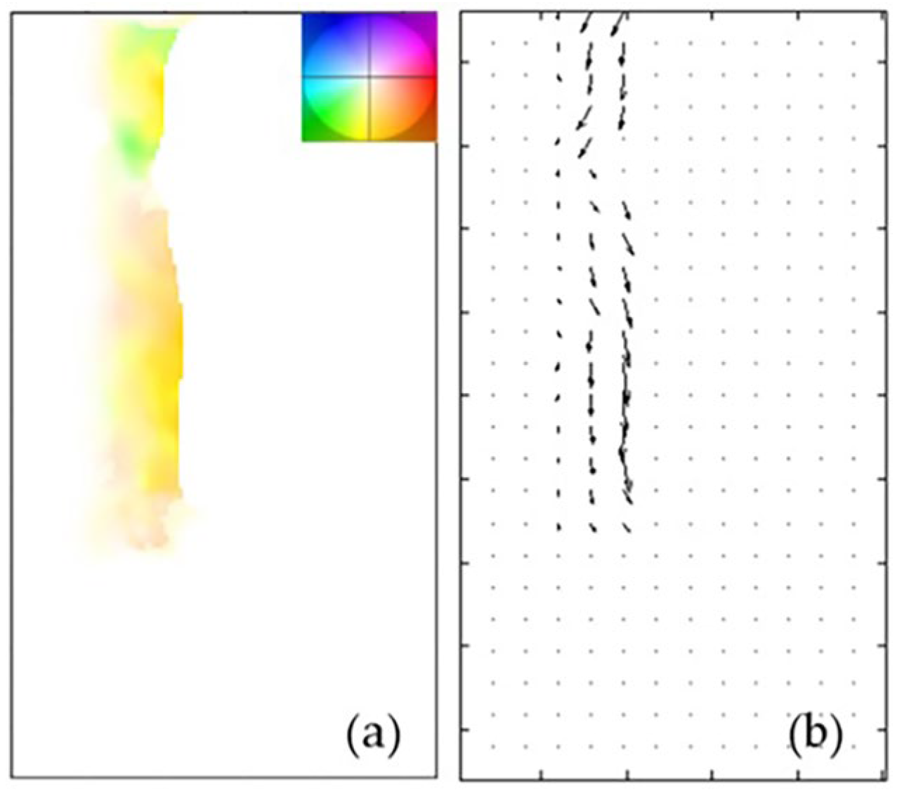
2. Optical Flow
2.1. Limitations of the Classical Horn–Schunck Model
2.2. Improvement of HS Model
2.2.1. Direct Photometric Difference Minimization
2.2.2. Charbonnier Penalty for Robustness
2.2.3. Coarse-to-Fine Warping Strategy
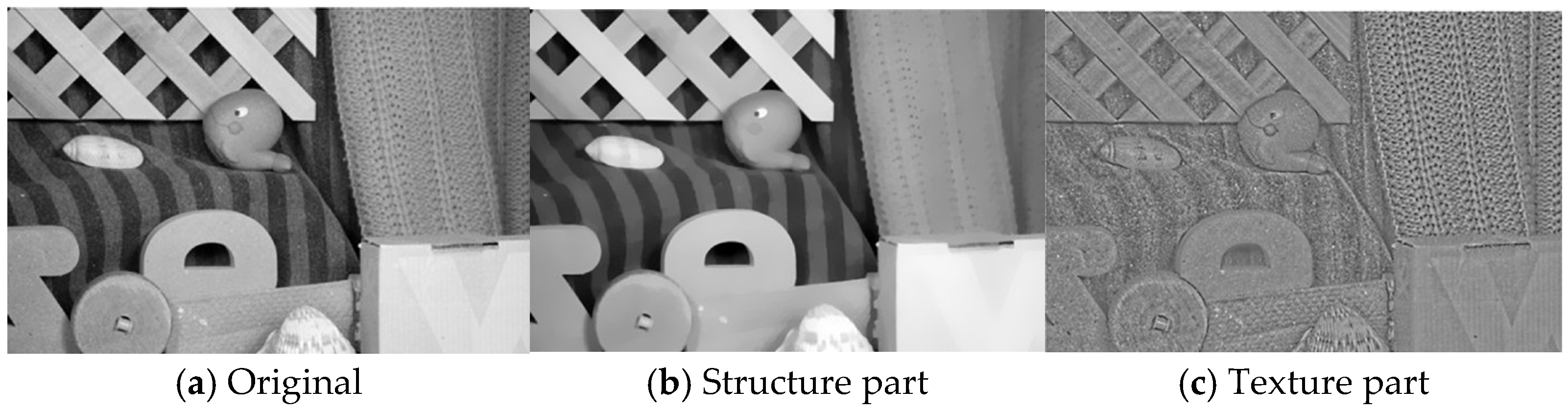
2.2.4. Structure and Texture Decomposition
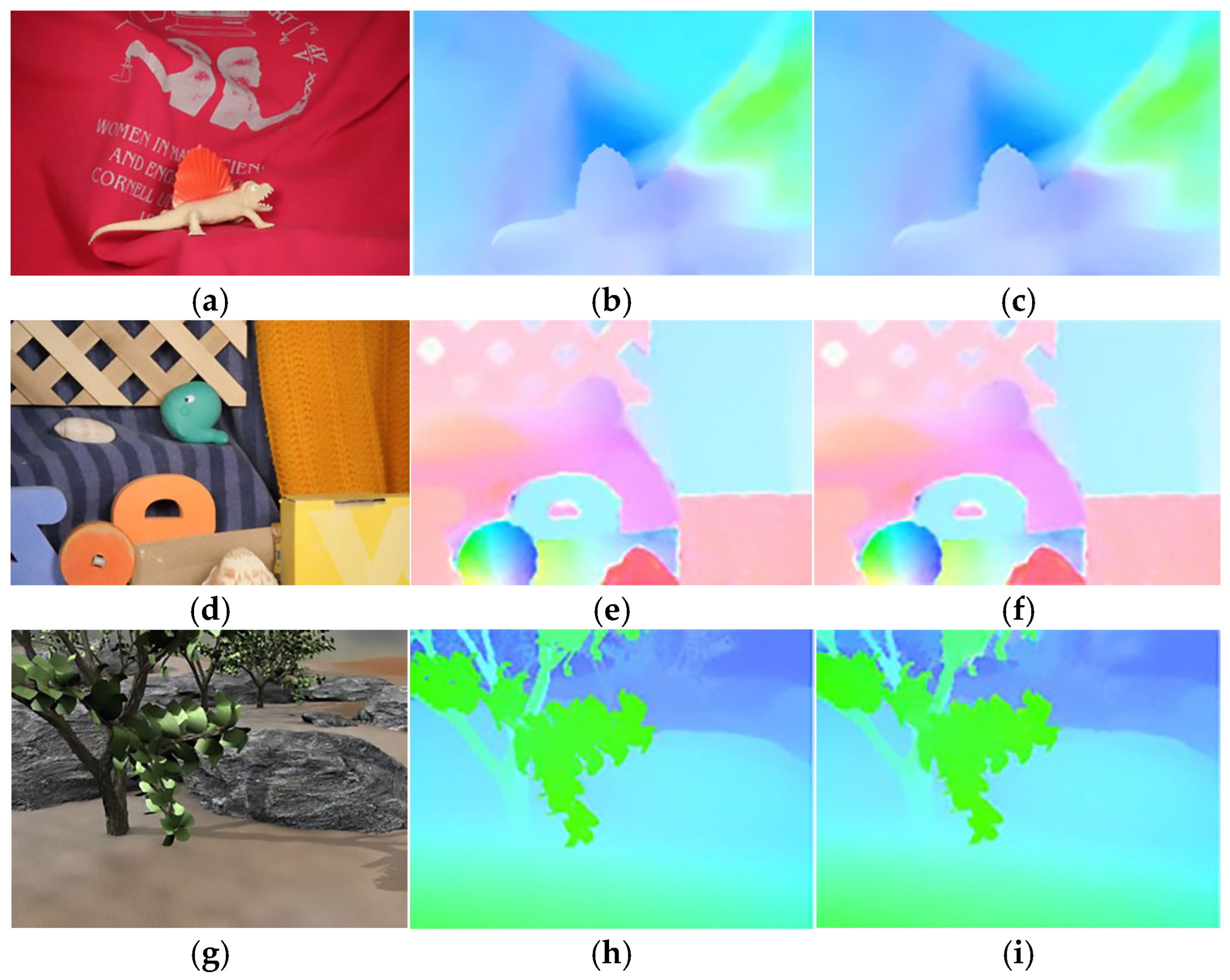
2.3. The Quantitative Accuracy of Improved HS Model
3. Chaotic Analysis
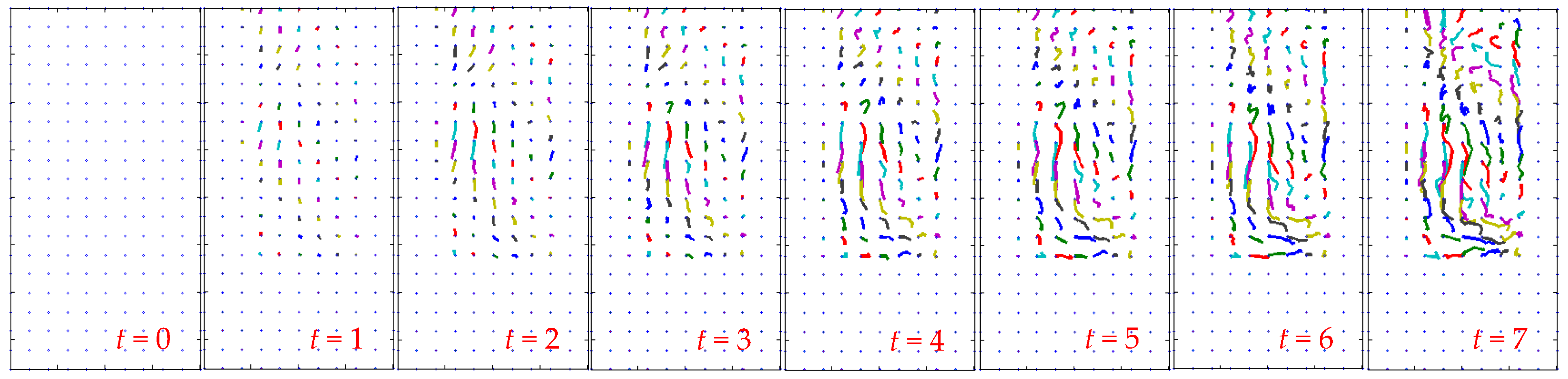
3.1. Streakline Computation
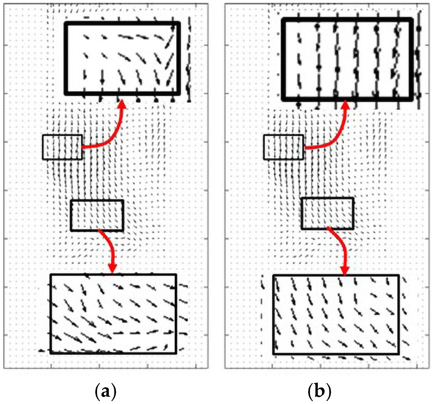
3.2. Streak Flow Computation Based on Streaklines
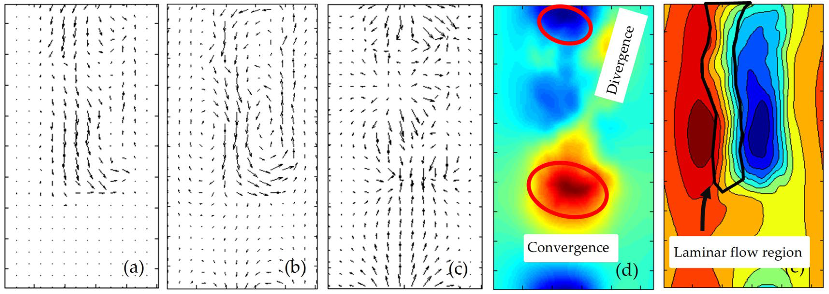
3.3. Potential Functions Based on the Streak Flow
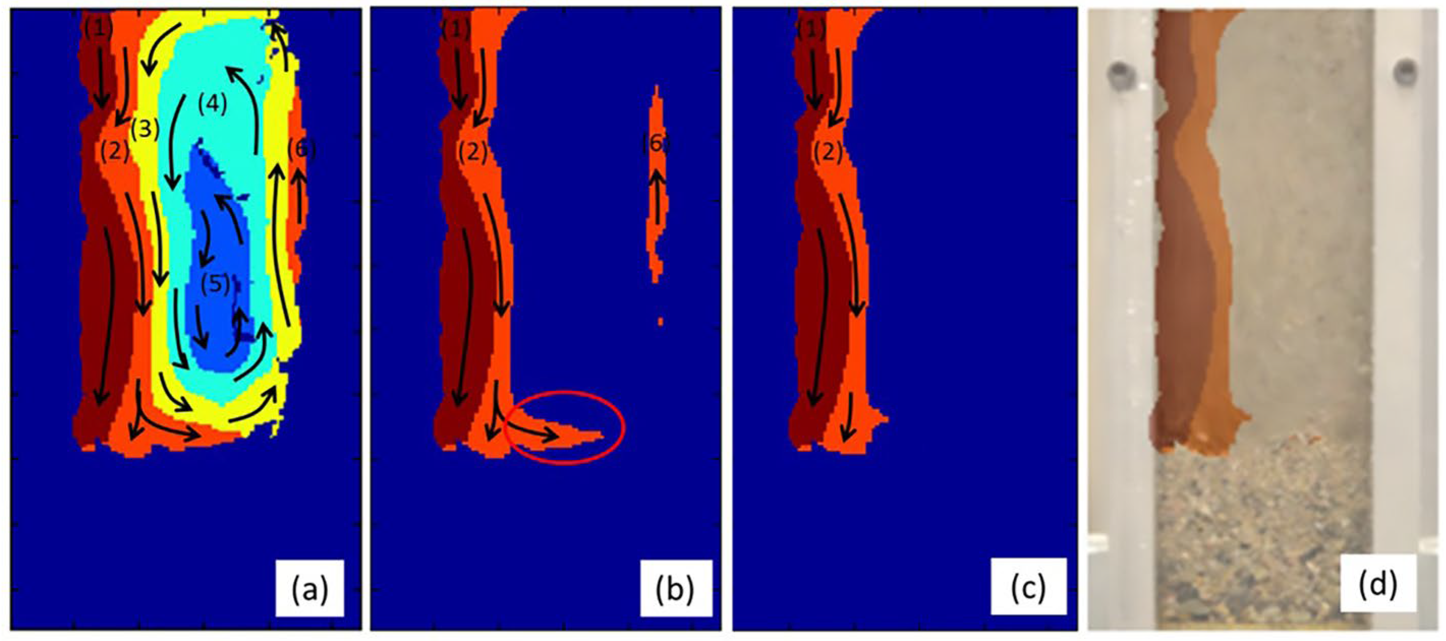
3.4. Chaotic Motion Analysis
4. Particle Size Estimation Based on the Laminar Flow Field
5. Experimental Results
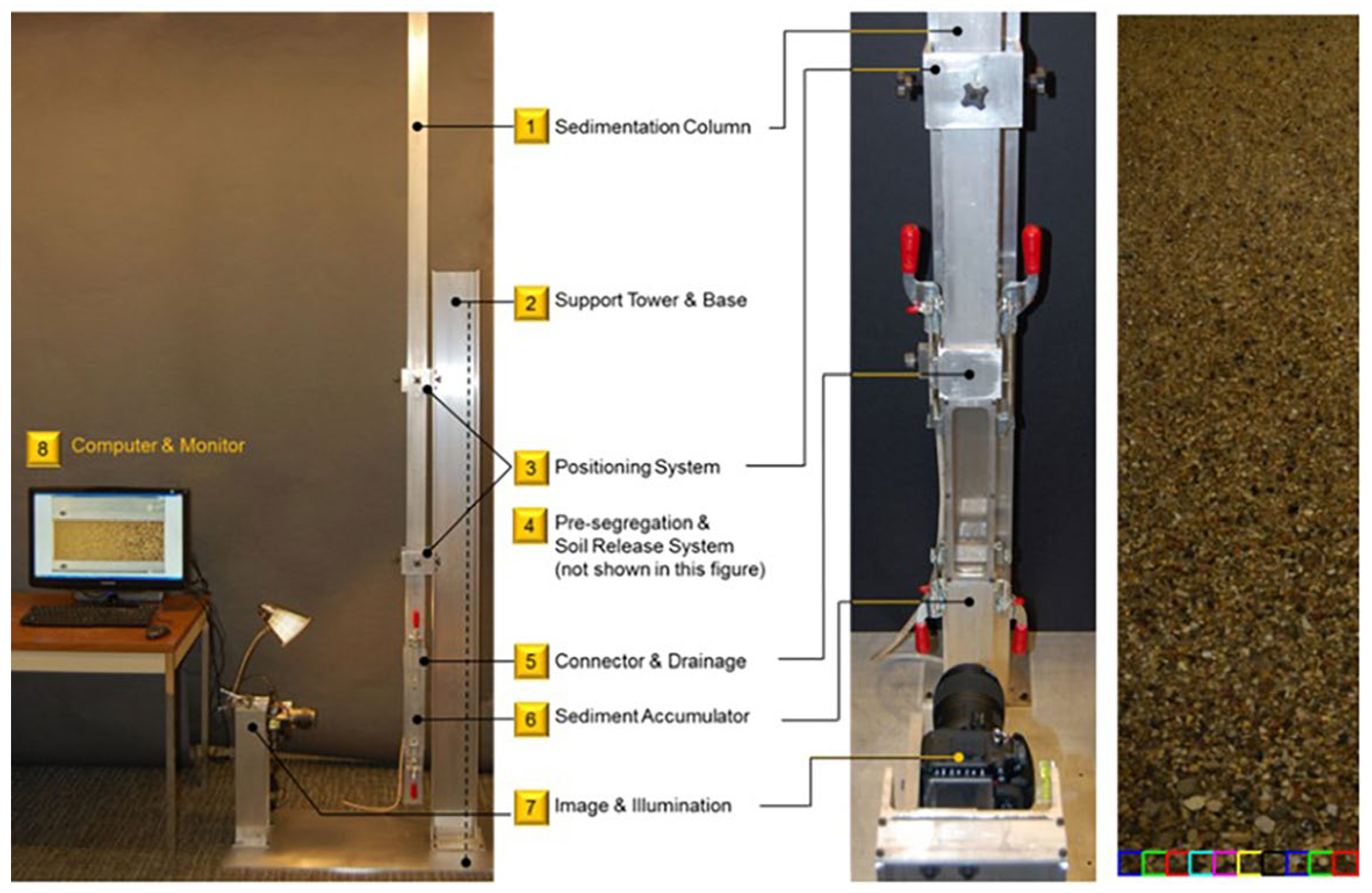
5.1. Experimental Setup and Data Acquisition
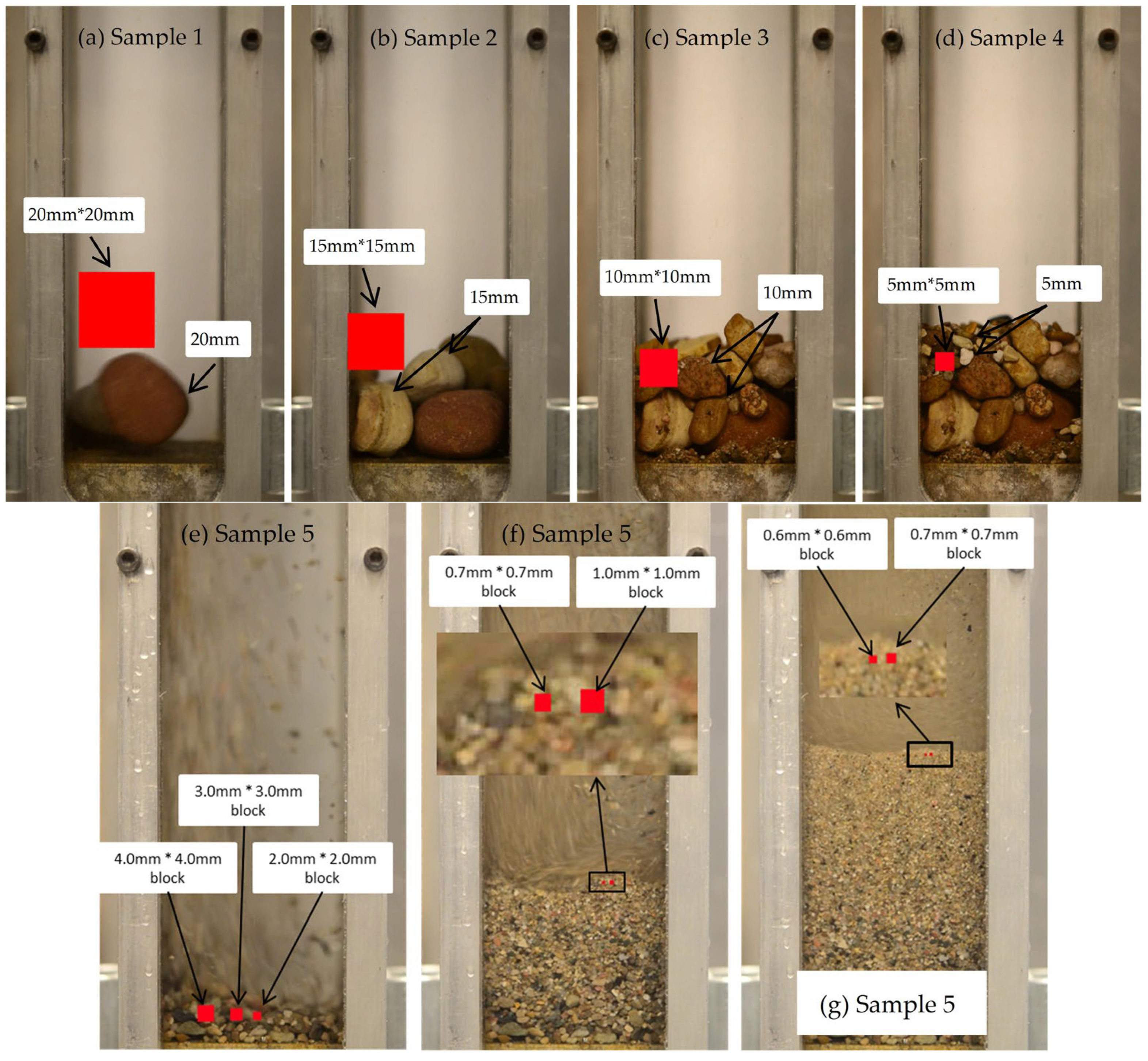
5.2. Particle Size Estimation for Uniform Samples
5.3. Particle Size Estimation for Fine Aggregate
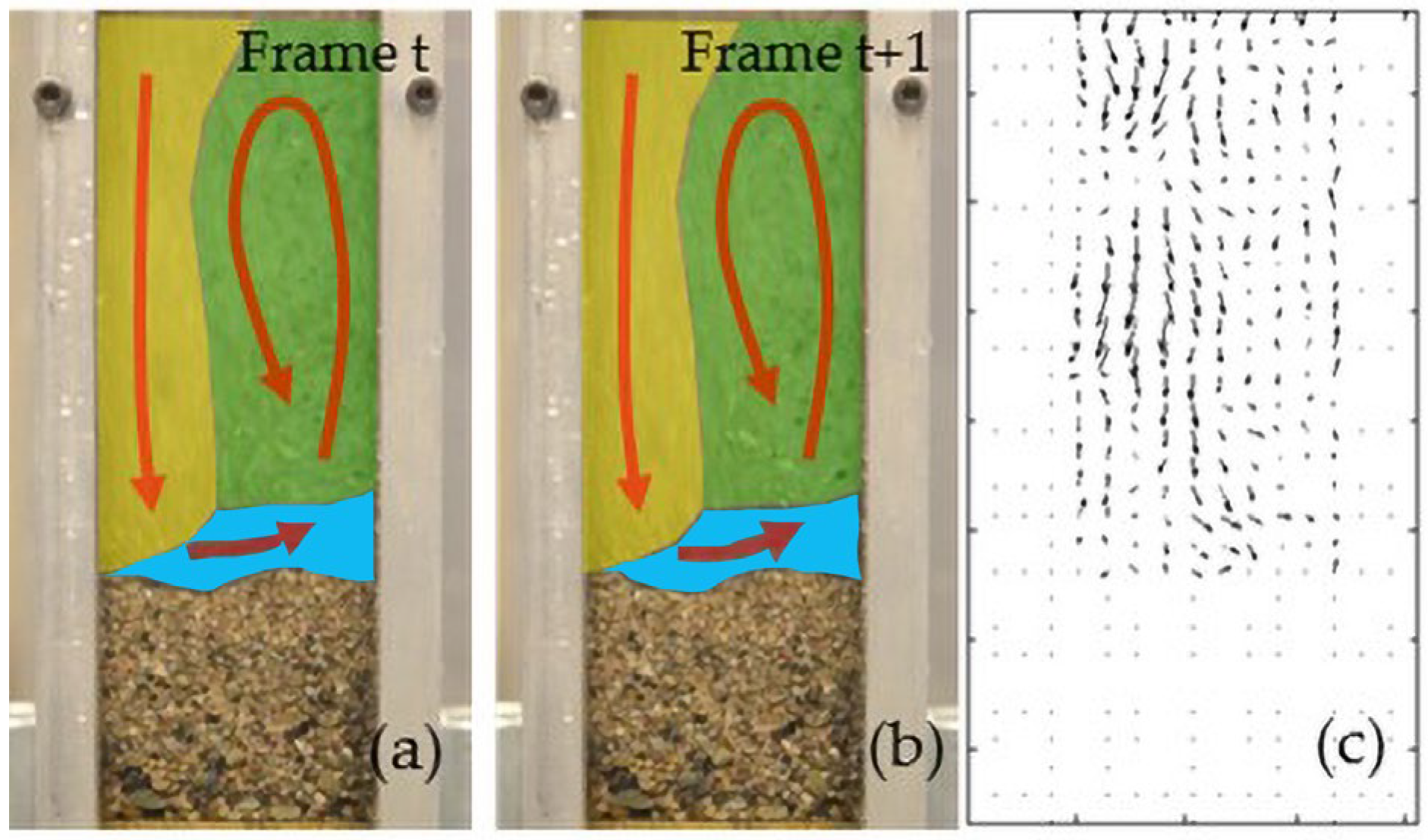
5.4. Robustness Evaluation Under Mixed Flow Conditions
5.5. Factors Affecting Optical Flow Performance
6. Conclusions and Future Research
6.1. Summary of Contributions
6.2. Limitations and Theoretical Scalability
6.3. Robustness Evaluation Under Mixed-Flow Conditions
6.4. Real-World Applications and Deployment Guidelines
Author Contributions
Funding
Data Availability Statement
Conflicts of Interest
References
- Kim, D.; Ha, S. Effects of particle size on the shear behavior of coarse grained soils reinforced with geogrid. Materials 2014, 7, 963–979. [Google Scholar] [CrossRef] [PubMed]
- Verma, G.; Kumar, B. Prediction of compaction parameters for fine-grained and coarse-grained soils: A review. Int. J. Geotech. Eng. 2020, 14, 970–977. [Google Scholar] [CrossRef]
- Xie, Y.; Yang, J.; Zheng, X.; Qu, T.; Zhang, C.; Fu, J. Effect of Particle Size Distributions (PSDs) on ground responses induced by tunnelling in dense coarse-grained soils: A DEM investigation. Comput. Geotech. 2023, 163, 105763. [Google Scholar] [CrossRef]
- Zhu, S.; Ye, H.; Yang, Y.; Ma, G. Research and application on large-scale coarse-grained soil filling characteristics and gradation optimization. Granul. Matter 2022, 24, 121. [Google Scholar] [CrossRef]
- Roy, S.; Bhalla, S.K. Role of geotechnical properties of soil on civil engineering structures. Resour. Environ. 2017, 7, 103–109. [Google Scholar]
- Mahawish, A.; Bouazza, A.; Gates, W.P. Effect of particle size distribution on the bio-cementation of coarse aggregates. Acta Geotech. 2018, 13, 1019–1025. [Google Scholar] [CrossRef]
- Afrazi, M.; Yazdani, M. Determination of the effect of soil particle size distribution on the shear behavior of sand. J. Adv. Eng. Comput. 2021, 5, 125–134. [Google Scholar] [CrossRef]
- Nagaraju, T.V.; Ravindran, G. Ground Improvement Techniques for Sustainable Engineering; Bentham Science Publishers Pte. Ltd.: Singapore, 2025. [Google Scholar]
- Patel, A. Geotechnical Investigations and Improvement of Ground Conditions; Woodhead Publishing: Kidlington, UK, 2019. [Google Scholar]
- Roque, A.J.; Paleologos, E.K.; O’Kelly, B.C.; Tang, A.M.; Reddy, K.R.; Vitone, C.; Mohamed, A.M.; Koda, E.; Goli, V.S.N.S.; Vieira, C.; et al. Sustainable environmental geotechnics practices for a green economy. Environ. Geotech. 2021, 9, 68–84. [Google Scholar] [CrossRef]
- Moreno-Maroto, J.M.; Alonso-Azcárate, J.; O’Kelly, B.C. Review and critical examination of fine-grained soil classification systems based on plasticity. Appl. Clay Sci. 2021, 200, 105955. [Google Scholar] [CrossRef]
- Erguler, Z.A. A quantitative method of describing grain size distribution of soils and some examples for its applications. Bull. Eng. Geol. Environ. 2016, 75, 807–819. [Google Scholar] [CrossRef]
- Budhu, M. Soil Mechanics and Foundations; John Wiley and Sons: Hoboken, NJ, USA, 2010. [Google Scholar]
- Mousa, A.; Youssef, T.A. Genesis of transitional behaviour in geomaterials: A review and gap analysis. Geomech. Geoengin. 2021, 16, 298–324. [Google Scholar] [CrossRef]
- Waters, S.G. Development of an Information System for Geotechnical Engineers Towards Improved Decision Making. Ph.D. Thesis, Central University of Technology, Bloemfontein, South Africa, 2022. [Google Scholar]
- Hryciw, R.D.; Ohm, H.S. Feasibility of Digital Imaging to Characterize Earth Materials; Report No. RC1557; Michigan Department of Transportation: Lansing, MI, USA, 2012.
- Kroetsch, D.; Wang, C. Particle size distribution. Soil Sampl. Methods Anal. 2008, 2, 713–725. [Google Scholar]
- Roostaei, M.; Hosseini, S.A.; Soroush, M.; Velayati, A.; Alkouh, A.; Mahmoudi, M.; Ghalambor, A.; Fattahpour, V. Comparison of various particle-size distribution-measurement methods. SPE Reserv. Eval. Eng. 2020, 23, 1159–1179. [Google Scholar] [CrossRef]
- Krawczykowski, D. Unification of particle size analysis results, part 1—Comparison of particle size distribution functions obtained by various measurement methods. Measurement 2024, 238, 115403. [Google Scholar] [CrossRef]
- Van der Meeren, P.; Dewettinck, K.; Saveyn, H. Particle Size Analysis; Food Science and Technology; Marcel Dekker: New York, NY, USA, 2004; Volume 138, p. 1805. [Google Scholar]
- Ulusoy, U. A review of particle shape effects on material properties for various engineering applications: From macro to nanoscale. Minerals 2023, 13, 91. [Google Scholar] [CrossRef]
- Xiao, Y.; Peng, Y.; Wang, M.; Ning, Y.; Zhou, Y.; Kong, K.; Long, Y. A novel method for predicting coarse aggregate particle size distribution based on Segment Anything model and machine learning. Constr. Build. Mater. 2024, 429, 136429. [Google Scholar] [CrossRef]
- Zhang, R.; Li, K.; Yu, F.; Zhang, H.; Gao, Z.; Huang, Y. Aggregate particle identification and gradation analysis method based on the deep learning network of Mask R-CNN. Mater. Today Commun. 2023, 35, 106269. [Google Scholar] [CrossRef]
- Ohm, H.S.; Hryciw, R.D. Particle Shape Determination in a Sedimaging Device. In Proceedings of the World Congress on Advances in Civil, Environmental and Materials Research (ACEM’12), Seoul, Republic of Korea, 26–30 August 2012; pp. 637–643. [Google Scholar]
- Shin, S.; Hryciw, R.D. Wavelet analysis of soil mass images for particle size determination. J. Comput. Civ. Eng. 2004, 18, 19–27. [Google Scholar] [CrossRef]
- Jung, Y.; Hryciw, R.D.; Elsworth, D. Vision cone penetrometer calibration for soil grain size. In Proceedings of the 3rd International Conference on Site Characterization ISC, Taipei, Taiwan, 1–4 April 2008; Volume 3, pp. 1303–1308. [Google Scholar]
- Hryciw, R.D.; Jung, Y. Three-Point Imaging Test for AASHTO Soil Classification. Transp. Res. Rec. 2009, 2101, 27–33. [Google Scholar] [CrossRef]
- Hryciw, R.D.; Ohm, H.S.; Zhou, J. Theoretical basis for optical granulometry by wavelet transformation. J. Comput. Civ. Eng. 2015, 29, 04014050. [Google Scholar] [CrossRef]
- Gao, L.; Wang, D.; Miao, Y. A review of two-dimensional image-based technologies for size and shape characterization of coarse-grained granular soils. Powder Technol. 2024, 120115. [Google Scholar] [CrossRef]
- Horn, B.K.; Schunck, B.G. Determining optical flow. Artif. Intell. 1981, 17, 185–203. [Google Scholar] [CrossRef]
- Lucas, B.D.; Kanade, T. An iterative image registration technique with an application to stereo vision. In Proceedings of the IJCAI’81: 7th International Joint Conference on Artificial Intelligence, Vancouver, BC, Canada, 24–28 August 1981; Volume 2, pp. 674–679. [Google Scholar]
- Brox, T.; Bruhn, A.; Papenberg, N.; Weickert, J. High accuracy optical flow estimation based on a theory for warping. In Computer Vision-ECCV 2004, Proceedings of the 8th European Conference on Computer Vision, Prague, Czech Republic, 11–14 May 2004; Proceedings, Part IV 8; Springer: Prague, Czech Republic, 2004; pp. 25–36. [Google Scholar]
- Shi, S.; Zhang, D.; Zhang, C.; Chen, Z.; Feng, C.; Fan, B. Large displacement optical flow estimation based on robust interpolation of sparse correspondences. IEEE Access 2020, 8, 227360–227372. [Google Scholar] [CrossRef]
- Danilova, M.; Dvurechensky, P.; Gasnikov, A.; Gorbunov, E.; Guminov, S.; Kamzolov, D.; Shibaev, I. Recent theoretical advances in non-convex optimization. In High-Dimensional Optimization and Probability: With a View Towards Data Science; Springer International Publishing: Cham, Switzerland, 2022; pp. 79–163. [Google Scholar]
- Fotopoulos, G.B.; Popovich, P.; Papadopoulos, N.H. Review Non-convex Optimization Method for Machine Learning. arXiv 2024, arXiv:2410.02017. [Google Scholar]
- Bruhn, A.; Weickert, J.; Schnörr, C. Lucas/Kanade meets Horn/Schunck: Combining local and global optic flow methods. Int. J. Comput. Vis. 2005, 61, 211–231. [Google Scholar] [CrossRef]
- Alfarano, A.; Maiano, L.; Papa, L.; Amerini, I. Estimating optical flow: A comprehensive review of the state of the art. Comput. Vis. Image Underst. 2024, 249, 104160. [Google Scholar] [CrossRef]
- Wang, J.; Zhong, Y.; Dai, Y.; Zhang, K.; Ji, P.; Li, H. Displacement-invariant matching cost learning for accurate optical flow estimation. Adv. Neural Inf. Process. Syst. 2020, 33, 15220–15231. [Google Scholar]
- Wedel, A.; Pock, T.; Zach, C.; Bischof, H.; Cremers, D. An improved algorithm for tv-l 1 optical flow. In Statistical and Geometrical Approaches to Visual Motion Analysis, Proceedings of the International Dagstuhl Seminar, Dagstuhl Castle, Germany, 13–18 July 2008; Revised Papers; Springer: Berlin/Heidelberg, Germany, 2009; pp. 23–45. [Google Scholar]
- Li, T.; Chang, H.; Wang, M.; Ni, B.; Hong, R.; Yan, S. Crowded scene analysis: A survey. IEEE Trans. Circuits Syst. Video Technol. 2014, 25, 367–386. [Google Scholar] [CrossRef]
- Wu, S.; Moore, B.E.; Shah, M. Chaotic invariants of lagrangian particle trajectories for anomaly detection in crowded scenes. In Proceedings of the 2010 IEEE Computer Society Conference on Computer Vision and Pattern Recognition, San Francisco, CA, USA, 13–18 June 2010; IEEE: Piscataway, NJ, USA, 2010; pp. 2054–2060. [Google Scholar]
- Ong, K.E.; Ng, X.L.; Li, Y.; Ai, W.; Zhao, K.; Yeo, S.Y.; Liu, J. Chaotic world: A large and challenging benchmark for human behavior understanding in chaotic events. In Proceedings of the IEEE/CVF International Conference on Computer Vision, Paris, France, 2–6 October 2023; pp. 20213–20223. [Google Scholar]
- Hu, W.; Xiao, X.; Fu, Z.; Xie, D.; Tan, T.; Maybank, S. A system for learning statistical motion patterns. IEEE Trans. Pattern Anal. Mach. Intell. 2006, 28, 1450–1464. [Google Scholar]
- Ihaddadene, N.; Djeraba, C. Real-time crowd motion analysis. In Proceedings of the 2008 19th International Conference on Pattern Recognition, Tampa, FL, USA, 8–11 December 2008; IEEE: Piscataway, NJ, USA, 2008; pp. 1–4. [Google Scholar]
- Ali, S.; Shah, M.A. lagrangian particle dynamics approach for crowd flow segmentation and stability analysis. In Proceedings of the 2007 IEEE Conference on Computer Vision and Pattern Recognition, Minneapolis, MN, USA, 17–22 June 2007; IEEE: Piscataway, NJ, USA, 2007; pp. 1–6. [Google Scholar]
- Palmieri, F. Network anomaly detection based on logistic regression of nonlinear chaotic invariants. J. Netw. Comput. Appl. 2019, 148, 102460. [Google Scholar] [CrossRef]
- Zhou, J.T.; Du, J.; Zhu, H.; Peng, X.; Liu, Y.; Goh, R.S.M. Anomalynet: An anomaly detection network for video surveillance. IEEE Trans. Inf. Forensics Secur. 2019, 14, 2537–2550. [Google Scholar] [CrossRef]
- Song, L.; Jiang, F.; Shi, Z.; Molina, R.; Katsaggelos, A.K. Toward dynamic scene understanding by hierarchical motion pattern mining. IEEE Trans. Intell. Transp. Syst. 2014, 15, 1273–1285. [Google Scholar] [CrossRef]
- Ni, J.; Chen, Y.; Tang, G.; Shi, J.; Cao, W.; Shi, P. Deep learning-based scene understanding forautonomous robots: A survey. Intell. Robot. 2023, 3, 374–401. [Google Scholar] [CrossRef]
- Mehran, R. Analysis of Behaviors in Crowd Videos. Doctoral Dissertation, University of Central Florida, Orlando, FL, USA, 2011. [Google Scholar]
- Corpetti, T.; Mémin, É.; Pérez, P. Dense estimation of fluid flows. IEEE Trans. Pattern Anal. Mach. Intell. 2002, 24, 365–380. [Google Scholar] [CrossRef]
- Amato, U.; Antoniadis, A.; De Feis, I.; Gijbels, I. Penalised robust estimators for sparse and high-dimensional linear models. Stat. Methods Appl. 2021, 30, 1–48. [Google Scholar] [CrossRef]
- Rathod, S.; Sahni, M.; Merigo, J.M. Development and Applications of Penalty-Based Aggregation Operators in Multicriteria Decision Making. Int. J. Intell. Syst. 2025, 2025, 6069158. [Google Scholar] [CrossRef]
- Yang, Y.; Liu, T.; Wang, Y.; Zhou, J.; Gan, Q.; Wei, Z.; Zhang, Z.; Huang, Z.; Wipf, D. Graph neural networks inspired by classical iterative algorithms. In Proceedings of the International Conference on Machine Learning, PMLR, Online, 18–24 July 2021; pp. 11773–11783. [Google Scholar]
- Shah, S.T.H.; Xuezhi, X. Traditional and modern strategies for optical flow: An investigation. SN Appl. Sci. 2021, 3, 289. [Google Scholar] [CrossRef]
- Chen, Q.; Poullis, C. Motion estimation for large displacements and deformations. Sci. Rep. 2022, 12, 19721. [Google Scholar] [CrossRef] [PubMed]
- Weijer, W.; De Ruijter, W.P.; Sterl, A.; Drijfhout, S.S. Response of the Atlantic overturning circulation to South Atlantic sources of buoyancy. Glob. Planet. Change 2002, 34, 293–311. [Google Scholar] [CrossRef]
- Mileva, E. The Impact of Capital Flows on Domestic Investment in Transition Economies; ECB Working Paper No. 871; European Central Bank: Frankfurt am Main, Germany, 2008. [Google Scholar]
- Baker, S.; Scharstein, D.; Lewis, J.P.; Roth, S.; Black, M.J.; Szeliski, R. A database and evaluation methodology for optical flow. Int. J. Comput. Vis. 2011, 92, 1–31. [Google Scholar] [CrossRef]
- Xu, L.; Jia, J.; Matsushita, Y. Motion detail preserving optical flow estimation. IEEE Trans. Pattern Anal. Mach. Intell. 2011, 34, 1744–1757. [Google Scholar]
- Lekien, F.; Marsden, J. Tricubic interpolation in three dimensions. Int. J. Numer. Methods Eng. 2005, 63, 455–471. [Google Scholar] [CrossRef]
- Riley, P. Attachment Theory and the Teacher-Student Relationship: A Practical Guide for Teachers, Teacher Educators and School Leaders; Routledge: Oxfordshire, UK, 2010. [Google Scholar]
- Landau, L.D.; Lifshitz, E.M. Course of Theoretical Physics; Elsevier: Amsterdam, The Netherlands, 2013. [Google Scholar]
- Batchelor, G.K. Mass transfer from small particles suspended in turbulent fluid. J. Fluid Mech. 1980, 98, 609–623. [Google Scholar] [CrossRef]


| Method | Grove2 | RubberWhale | Dimetrodon | Urban 2 | Average | |||||
|---|---|---|---|---|---|---|---|---|---|---|
| AAE | EPE | AAE | EPE | AAE | EPE | AAE | EPE | AAE | EPE | |
| Traditional HS ([30]) | 15.853 | 5.204 | 16.798 | 6.118 | 19.675 | 7.224 | 16.069 | 8.459 | 17.098 | 6.751 |
| Improved HS (This research) | 8.410 | 1.189 | 6.240 | 1.276 | 5.280 | 1.217 | 7.034 | 1.210 | 6.741 | 1.223 |
| Value | Sample 1 | Sample 2 | Sample 3 | Sample 4 |
|---|---|---|---|---|
| Range of five sizes (mm) | 19.2~22.0 | 15.0~15.9 | 12.8~8.0 | 4.4~5.2 |
| Final size (average) (mm) | 19.6 | 15.4 | 10.4 | 4.9 |
| True value (mm) | 20.0 | 15.0 | 10.0 | 5.0 |
| Absolute error (mm) | 0.4 | 0.4 | 0.4 | 0.1 |
| Relative error (%) | 2.0% | 2.7% | 4.0% | 2.0% |
| True value (mm) | 20.0 | 15.0 | 10.0 | 5.0 |
| Value | Sample 5 (Figure 13e) | Sample 5 (Figure 13f) | Sample 5 (Figure 13g) |
|---|---|---|---|
| Range of five sizes(mm) | 2.0~3.8 | 0.72~1.33 | 0.62~0.73 |
| Final size (average)(mm) | 2.9 | 0.87 | 0.66 |
| Observed true value(mm) | 2.0~4.0 (3.0 average) | 0.7~1.0 (0.85 average) | 0.5~0.7 (0.65 average) |
| Visual average (mm) | ~3.0 | ~0.85 | ~0.65 |
| Estimated error (mm) | ~0.1 | ~0.02 | ~0.01 |
| Sample | True Size (mm) | Mean Error (No Filter) | Mean Error (Filtered) | Std. Dev (No Filter) | Std. Dev (Filtered) |
|---|---|---|---|---|---|
| S1 | 20.0 | 1.2 mm | 0.4 mm | 1.7 mm | 1.1 mm |
| S2 | 15.0 | 0.8 mm | 0.3 mm | 1.2 mm | 0.8 mm |
| S3 | 10.0 | 0.6 mm | 0.2 mm | 0.9 mm | 0.6 mm |
| S4 | 5.0 | 0.3 mm | 0.1 mm | 0.6 mm | 0.4 mm |
| Average | — | 0.725 mm | 0.25 mm | 1.1 mm | 0.725 mm |
Disclaimer/Publisher’s Note: The statements, opinions and data contained in all publications are solely those of the individual author(s) and contributor(s) and not of MDPI and/or the editor(s). MDPI and/or the editor(s) disclaim responsibility for any injury to people or property resulting from any ideas, methods, instructions or products referred to in the content. |
© 2025 by the authors. Licensee MDPI, Basel, Switzerland. This article is an open access article distributed under the terms and conditions of the Creative Commons Attribution (CC BY) license (https://creativecommons.org/licenses/by/4.0/).
Share and Cite
Li, S.; Gao, L.; Zhang, B.; Liu, Z.; Zhang, X.; Guan, L.; Tang, H. Soil Particle Size Estimation via Optical Flow and Potential Function Analysis for Dam Seepage and Building Monitoring. Buildings 2025, 15, 1800. https://doi.org/10.3390/buildings15111800
Li S, Gao L, Zhang B, Liu Z, Zhang X, Guan L, Tang H. Soil Particle Size Estimation via Optical Flow and Potential Function Analysis for Dam Seepage and Building Monitoring. Buildings. 2025; 15(11):1800. https://doi.org/10.3390/buildings15111800
Chicago/Turabian StyleLi, Shuangping, Lin Gao, Bin Zhang, Zuqiang Liu, Xin Zhang, Linjie Guan, and Han Tang. 2025. "Soil Particle Size Estimation via Optical Flow and Potential Function Analysis for Dam Seepage and Building Monitoring" Buildings 15, no. 11: 1800. https://doi.org/10.3390/buildings15111800
APA StyleLi, S., Gao, L., Zhang, B., Liu, Z., Zhang, X., Guan, L., & Tang, H. (2025). Soil Particle Size Estimation via Optical Flow and Potential Function Analysis for Dam Seepage and Building Monitoring. Buildings, 15(11), 1800. https://doi.org/10.3390/buildings15111800