Article

From Density to Efficiency: Exploring Urban Building Use Efficiency in 35 Large Chinese Cities

1
Advanced Laser Technology Laboratory of Anhui Province, Hefei 230000, China
2
Department of Land Management, Zhejiang University, Hangzhou 310058, China
3
Department of Public Courses, Wuhan Institute of Shipbuilding Technology, Wuhan 430074, China
4
School of Architecture and Urban Planning, Huazhong University of Science and Technology, Wuhan 430074, China
5
College of Public Administration & Law, Fujian Agricultural and Forestry University, Fuzhou 350002, China
6
School of Public Policy & Management, China University of Mining and Technology, Xuzhou 221116, China
*
Author to whom correspondence should be addressed.
Buildings 2025, 15(11), 1803; https://doi.org/10.3390/buildings15111803
Submission received: 10 April 2025 / Revised: 11 May 2025 / Accepted: 22 May 2025 / Published: 24 May 2025
(This article belongs to the Section Building Energy, Physics, Environment, and Systems)

Abstract

Efficient urban land use is essential for sustainable urban growth. However, the efficiency of buildings in carrying urban functions remains poorly understood. A comprehensive approach for measuring urban building use efficiency (UBUE) and marginal effect was developed by quantifying the relationship between building volume and urban function. The intensity of urban function was calculated from nighttime light intensity, population density, and facility density. The UBUE at national and urban scales was assessed for 35 Chinese cities. Three significant findings emerge. First, UBUE shows significant spatial variation at national and urban scales, with a maximum disparity of 4.3 times among the 35 cities and a gradual decline along the urban–rural gradient within urban areas. Second, in cities in the western and northeastern areas, a smaller amount of urban function was generated per unit of newly constructed building volume, indicating that newly increased buildings are less efficient. Third, the scaling exponents of most cities were less than one, suggesting a marginal diminishing effect in the relationship between urban function and building volume. The marginal diminishing effect was more pronounced in economically developed cities. The comprehensive investigation of the relationship between urban function and building volume provides a scientific basis for land development allocation policies and urban growth regulation.

1. Introduction

With the continuous increase in the global urban population, cities have substantially expanded in recent decades [1,2]. The urban population share of the world population is expected to exceed 60% by 2030 and reach 75% by the middle of the 21st century [3]. This implies that the demand for urban land will continue to increase. Although built-up areas occupy only a small fraction of the global land area [4,5], their expansion has mainly occurred at the expense of fertile farmland, thereby sacrificing agricultural production capacity. Research suggests that unless substantial changes are made to ensure a sustainable lifestyle, the human population’s growth, coupled with increasing wealth, will drive a surge in demand for food and housing in the coming decades [6]. Meanwhile, land take per person has been increasing in most regions of the world, and the trend is expected to continue in the coming decades [7]. The SDG indicator 11.3.1 measures the ratio of land consumption to new population growth, which serves as an important indicator for assessing the achievement of inclusive and sustainable urbanization [8]. This implies that inefficient urban expansion on a large scale substantially threatens urban sustainability. Therefore, curbing the sprawl of urban built-up land by enhancing urban land use efficiency has become a major goal of land use policy for sustainable development worldwide [9].
To address the challenges posed by limited urban land and the need to carry the increasing urban functions on limited urban land, the adoption of upward growth characterized by intensively constructed buildings in three dimensions has become a major solution [10,11,12]. Urban function is regarded as the “urban load” imposed on urban land owing to urbanization [13], which encompasses the comprehensive performance of human activities [14,15]. A recent study revealed that due to the construction boom and infrastructure-focused development, China’s urban expansion is characterized more by “vertical” growth, with an increase in high-rise buildings, rather than “horizontal” growth [16]. Such urban growth transformation from horizontal to vertical in China is forced by the strict restrictions on newly increased construction land quota imposed by China’s central government. This is also regarded as a primary land use regulation implemented by local government aiming to curb urban sprawl. On this account, vertical growth with high-rise buildings becomes a significant carrier for the increasing urban function brought by the new urban population during the urbanization process [13].
Recent studies have also emphasized the correlation between intensive urban land use and the capacity to support urban functions [17,18,19]. The theoretical foundation of such research lies in the interplay between urban morphology and urban function. Both morphological and functional dimensions are widely employed to characterize the overall urban spatial structure [20]. The morphological dimension refers to the scale and spatial distribution of the physical built environment, while the functional dimension is generally regarded as a reflection of socioeconomic performance, encompassing elements such as economic vitality and the intensity of human activities within cities, as highlighted in urban vitality theory [19]. Intensive land use with high-density buildings appears to guarantee the accommodation of more urban functions within a unit area of urban built-up land. For example, Xia et al. (2020) investigated five megacities in China and revealed a significant spatial autocorrelation between urban land use intensity and urban function [21]. Another empirical study in the Yangtze River Delta region also identified a strongly coupled relationship between urban land use intensity and land use efficiency [22]. Consequently, urban planning and management practices worldwide have adopted diverse strategies to promote high-density development that accommodates population growth while curbing urban sprawl, such as compact city concepts, new urbanism, and smart growth [23,24].
Although a strong correlation exists between urban morphology and urban function, functional changes do not always stem from morphological transformations, particularly in the context of China [25]. Land urbanization in China has progressed significantly faster than population urbanization, primarily due to local governments’ heavy reliance on land transfer revenues as a key source of fiscal income [26]. This mismatch between urban morphology and function increases the risk of building resource underutilization and often leads to vacant buildings, accompanied by shrinking commercial activity and a sparse population in newly developed urban areas. This phenomenon is driven by overdevelopment and inadequate planning, which is also called “ghost cities” [27].
However, existing literature concerning urban land use efficiency has failed to investigate and explain the urban function carrying efficiency of the vertical built-up environment. Buildings are the matrix and major elements of the urban landscape, which play a significant role as shelters for socioeconomic vitality [21,28]. The underlying assumption that intensive urban land development ensures land use efficiency is that dense building volume necessarily accommodates more urban functions. In fact, they largely overlooked the risk of inefficient use of buildings. Most scholars define urban land use efficiency as the ratio between urban area expansion (land consumption) and economic gain, following the concept of input–output relation [29,30]. Studies in this vein assess economic density according to the GDP in the unit area of built-up land [31,32]. Such measurements of urban land use efficiency takes the production value of the building construction industry into account of the “output” in urban land use efficiency calculations, which takes a considerable proportion of GDP [33]. Correspondingly, the amount of vertical built-up environment is regarded as an output element rather than an input element in traditional urban land use efficiency measurement. On this occasion, the inefficient utilization of intensive buildings would still be investigated as an extensive output in the traditional measurement of land use efficiency. This paradox indicates a defect in current studies of urban land use efficiency theory, which mistakenly regard the vertical built-up environment as a kind of economic output, while it actually plays the role of an urban function carrier.
Therefore, this study examined the relationship between the urban vertical built-up environment and urban functions among different cities at the national scale and across different locations within urban areas. The building volume density (BVD), determined by building footprint and building height, is employed as a significant measurement of the urban vertical built-up environment [22]. Specifically, we expressed three research questions: (1) What is the spatial heterogeneity pattern of the current amount of urban function carried by per unit of building volume in different geographical locations? (2) How much difference does the growth of per unit of building volume bring in terms of newly increased urban functions in different geographical locations? (3) What is the marginal effect of urban function on building volume growth in different geographical locations?
To address these questions, we first introduced the concept of urban building use efficiency (UBUE), defined as the ratio of urban function intensity (UFI) to building volume density (BVD). Drawing on urban vitality theory [19,34], UFI was constructed from multiple datasets: population density, point-of-interest (POI) density, and nighttime light (NTL) intensity. These metrics collectively capture the comprehensive performance of human activities closely linked to urban form’s physical structures. Specifically, population density serves as a fundamental micro-level driver of social processes. High density within confined geographic areas fosters diverse interactions, establishing prerequisites for interpersonal engagement [35,36]. POI facilities, meanwhile, meet socioeconomic demands by providing services that streamline production, circulation, and consumption [37]. NTL intensity has been widely validated as a proxy for measuring human activity intensity and spatial distribution [38,39]. Second, we employed the slope value from linear regression models of BVD and UFI to quantify how urban function increases with additional building volume. Third, scaling exponents derived from power function fits were used to characterize changes in urban function increments per unit of building volume growth.
The rest of the paper is organized as follows. Section 2 outlines the data collection and methodology of the study. Section 3 presents the empirical results. Section 4 discusses the results of the evaluation of UBUE indicators. Section 5 summarizes the main findings and presents the major contributions and limitations of the study.

2. Data Collection and Research Methodology
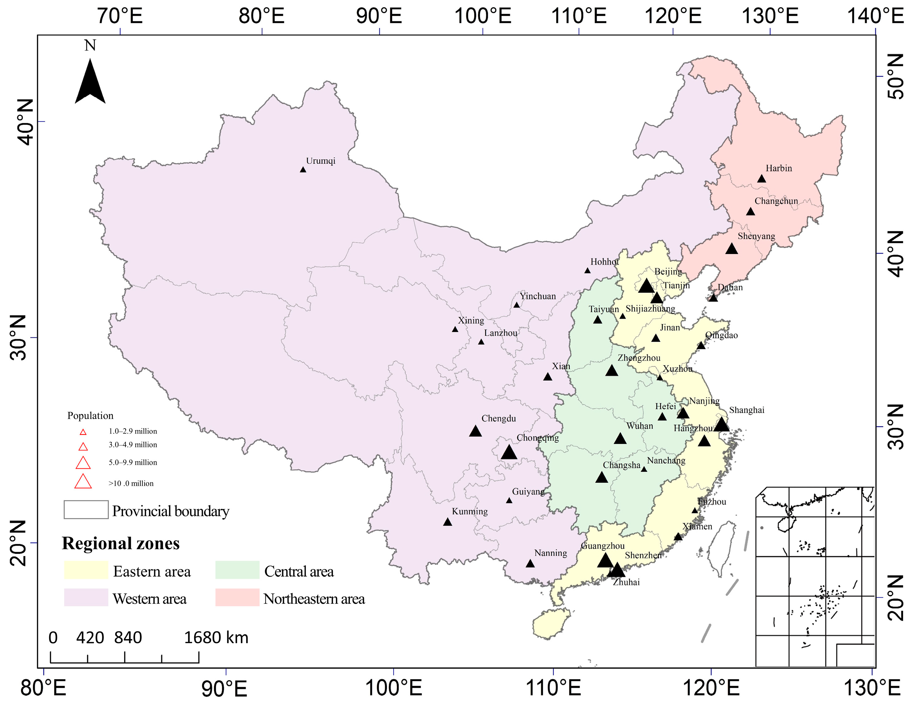
2.1. Study Area

To identify the spatial heterogeneity of UBUE at the national scale, we selected 35 cities located in different regions, including the eastern, central, western, and northeastern areas of China (Figure 1) [40]. These selected cities have experienced rapid urbanization and substantial growth in the number of tall buildings in recent decades [41,42]. According to the official standards for classifying the size of cities in China, the 35 cities were divided into four sizes based on their urban population: type II big cities, type I big cities, supercities, and megacities.

2.2. Data Preprocessing

2.2.1. Data Sources

The urban areas of these cities in 2018 were identified according to the high-resolution (30 m) maps of global artificial impervious areas, an open-source database published by Gong et al. (2020) [43]. The geographical scopes of the urban areas were mapped according to the landscape of artificial impervious areas. We clipped the urban area according to the administrative boundaries to retrieve the statistical areas of the selected cities. The urban areas of these cities ranged from 301 km2 to 3885 km2.
Consequently, we built a fishnet for the urban area with 1 km2 grids to identify the average values of the relevant indicators, i.e., BVD, population density, POI density, and NTL intensity. Specifically, the building volume data were provided by Wu (2023) with a resolution of 10 m [44]. The building volume was retrieved from building height and footprint information, which achieved strong correlations with real observations at the national scale (RMSE = 6.1 m, MAE = 5.2 m, R = 0.77). The open-access WorldPop 100M population grid dataset was applied to measure the urban population with a high resolution of 100 m. A POI dataset containing nine types of functional facilities was applied to represent urban facilities that are closely related to human socioeconomic activities (Table 1) [45,46]. Global National Polar-orbiting Partnership Visible Infrared Imaging Radiometer Suite data were used to reflect stable NTL intensity. These data have previously been widely used to assess regional economic development [37,38]. All data with varying spatial resolutions were resampled using the 1 km2 grids. In addition, GDP and public budget expenditure data for the urban areas were collected from the official Chinese urban construction statistical yearbook. Specifically, these two indicators which reflect the intensity of urban fixed-asset investment, were collected one to three years earlier than the other datasets. This is because we considered the time-lag effect of fixed-asset investment on both socioeconomic development and the urban built environment.

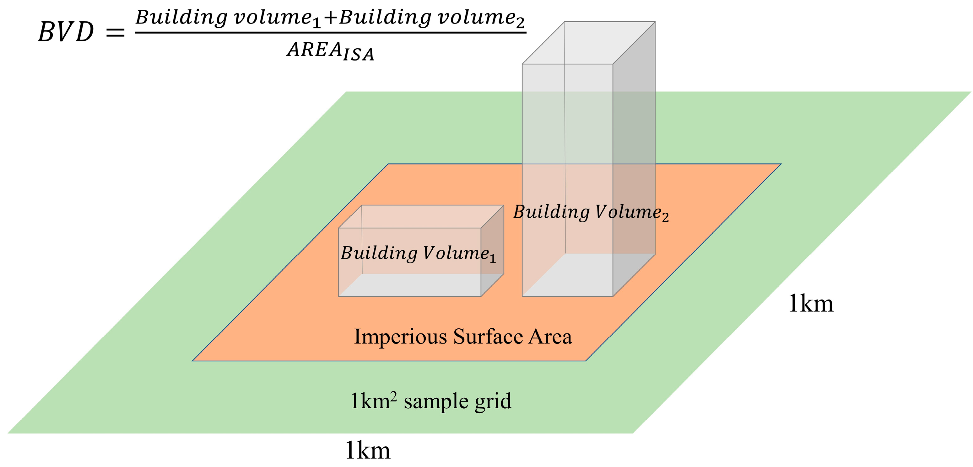
2.2.2. Identification of UBUE

We used population density and POI density to reflect residential function and facility service concerning urban function. Meanwhile, we employed NTL data to reflect the usage intensity of buildings at night, which to some extent also reflected the duration of building usage. These three factors were applied to measure the diverse human activities carried by buildings. Consequently, the BVD, population density, POI density, and NTL intensity of all the sample grids within urban areas were calculated. The quantification method of each criterion for a certain evaluation unit was as follows:
B V D = i = 1 n B V i B L
where BVD represents the average BVD of the sample grid (i.e., the ratio of the accumulated building volume to the area of built-up land); BVi is the building volume of the i-th pixel with a resolution of 10 m; n is the total number of building volume pixels within the sample grids; and B L is the corresponding built-up land area (Equation (1), Figure 2).
P O P d e n s = n i P O P i B L
where P O P d e n s represents the average population density of the sample grid (i.e., the ratio of the accumulated population to the area of built-up land); P O P i is the population of the i-th pixel with a scale of 100 × 100 m, and n is the total number of population pixels within the sample grids (Equation (3)).
P O I d e n s = P O I B L
where P O I d e n s represents the facility density of the built-up area (i.e., the ratio of the total POI amount to the area of built-up land (Equation (3)).
N T L i n t = n i L i n
where N T L i n t is the average nighttime illumination intensity of the sample grid (i.e., the ratio of accumulated nighttime illumination intensity to the pixel number); L i represents nighttime illumination intensity, measured by the radiance value of the i-th pixel, and n is the total NTL pixel number within the sample grid (Equation (4)).
We defined UBUE as the integrated urban function carried by a unit of building volume. Therefore, UBUE was equal to the ratio of UFI to the BVD of the sample grid. The measurement of UFI was a synthesis of P O P d e n s , P O I d e n s , and N T L i n t . The normalized weighted values of these indicators were calculated. Then, the entropy weight method was applied to guarantee the objectivity of the weight coefficients of the three indicators [42]. The entropy weight method employs information entropy to evaluate the information content and variability of each indicator. Specifically, greater variability in an indicator implies higher information content, thereby justifying a higher assigned weight. The calculation process is outlined as follows:
For each grid cell i and indicator j, raw values_ x i j were normalized using the min–max method.
p i j = x i j min ( x j ) max ( x j ) min ( x j )
The normalized values were transformed into a proportion matrix, with n denoting the total number of spatial grid cells.
f i j = p i j i = 1 n p i j
The entropy e j of each indicator was calculated using:
e j = 1 In ( n ) i = 1 n In ( f i j )
The diversification degree d j of each indicator was derived as:
d j = 1 e j
The final weight w j of each indicator was computed by normalizing the diversification degrees:
w j = d j j = 1 m d j
By employing the weights retrieved by the entropy weight method, we built the following UFI formula.
U F I = 0.354 × P D s t + 0.446 × P O I s t + 0.200 × N T L s t
where POPst, POIst, and NTLst are the standard values of these indicators.
Then, we calculated UBUE from the ratio of UFI and BVD as follows:
U B U E i = U F I i B V D i
where U B U E i represents the UBUE of the i-th sample grid; and U F I i and B V D i represent the UFI and BVD of the i-th pixel, respectively. The UBUE for all the sample grids was calculated according to Equation (6). The UBUE of each city was based on the average gridded UBUE. The independent samples t-test was used to compare the differences in UBUE across different urban buffers and regions. To identify the UBUE variation on urban–rural gradient, we selected the central business district (CBD) as it existed in 1990 as the center point for the concentric ring buffers, following the approach adopted in previous studies [50].

2.3. The Power Function and Linear Function Fitting

Scaling laws inherently characterize power-law relationships. Substantial evidence demonstrates scale invariance in urban systems across spatial, hierarchical, and size dimensions [51,52,53]. This functional form has been widely utilized in urban studies to quantify the relationship between urban population and diverse urban morphological attributes. Given the potential nonlinearity in the BVD–UFI relationship arising from marginal effect changes, the scaling law was employed to quantify their relationship in the form of a power law. The scaling law builds a unified framework to uncover how the quantitative attributes of buildings are related to their urban function [54,55]. The function of the scaling law was as follows (Equation (7)):
Y = Y 0 N β
where Y is the UFI, N is BVD, Y 0 is a parameter, and β is the scaling exponent. The scaling exponent (β) represents the correlation between BVD and UFI. If β is <1, the UFI increases more slowly than the BVD from a low-density city to a compact one, resulting in a sub-linear scaling relationship between the current BVD and UFI.
We further applied a linear regression to measure the reaction of UFI to variation in BVD (Equation (8)).
Y = α × N + ε
where ε is a parameter and α is the slope value of the linear regression model. The coefficient α represents the UFI increase triggered by the increase in BVD. It also reflects the degree of variation in UFI at different values of BVD.

2.4. Scale-Adjusted Metropolitan Indicator (SAMI)

The SAMI was used to evaluate UBUE at the national scale taking its nonlinear relationship into consideration. Mathematically, SAMI is the residual of the deviation of the observed UFI value from the expected value [45], and it is an indicator of the advantages and disadvantages of using the local UBUE at the national scale. A positive value of SAMI indicated that the observed local UFI was larger than the expected value according to the power function fitting between BVD and UFI at the national scale (Equation (9)).
S A M I i = log Y i log ( Y 0 N i β )
where Y i is the observed UFI of grid i, N i is the BVD of grid I, Y 0 and β are the same parameters as in Equation (7). We calculated SAMI for all the 1 km2 grids in the urban areas of the selected cities.

3. Results

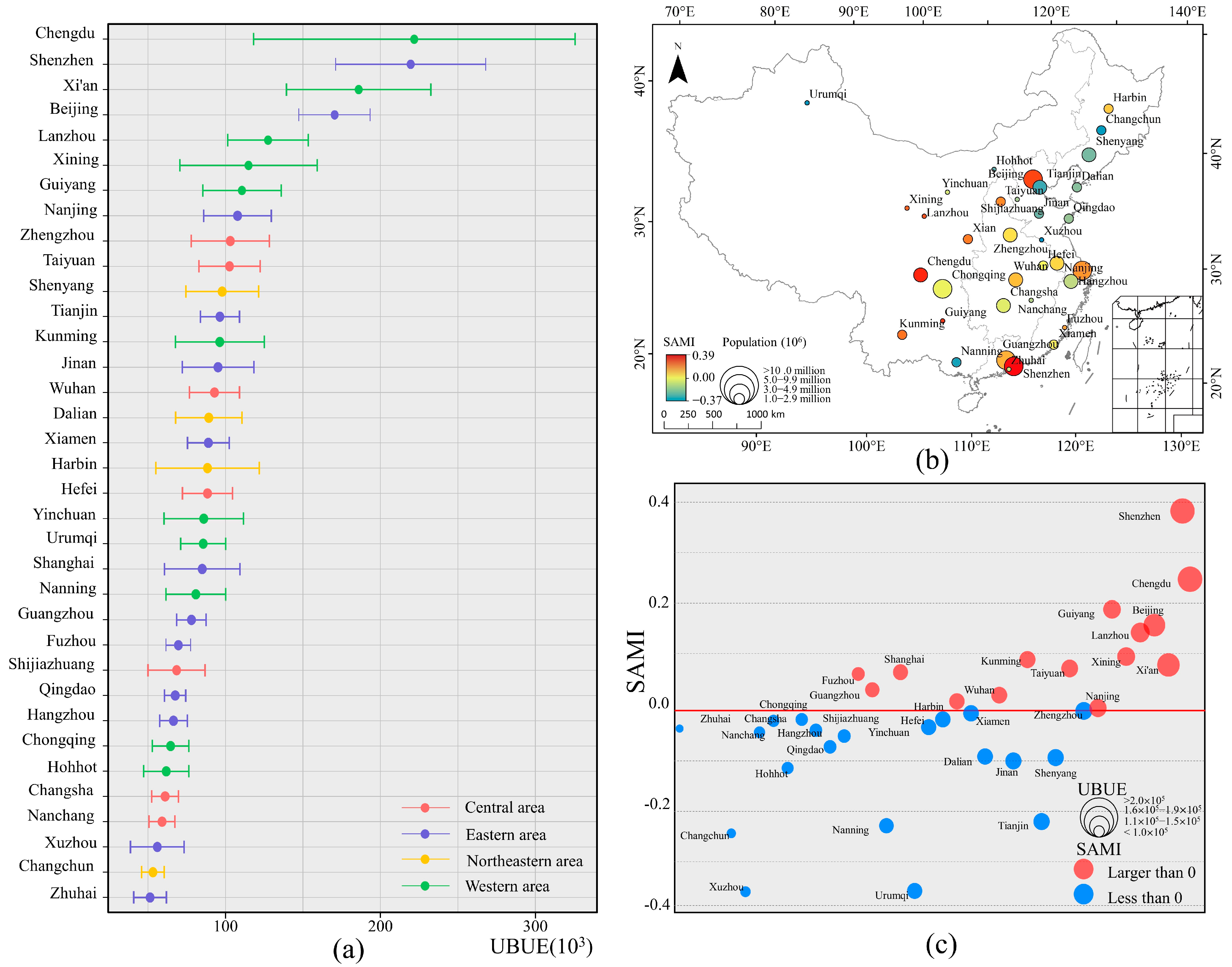
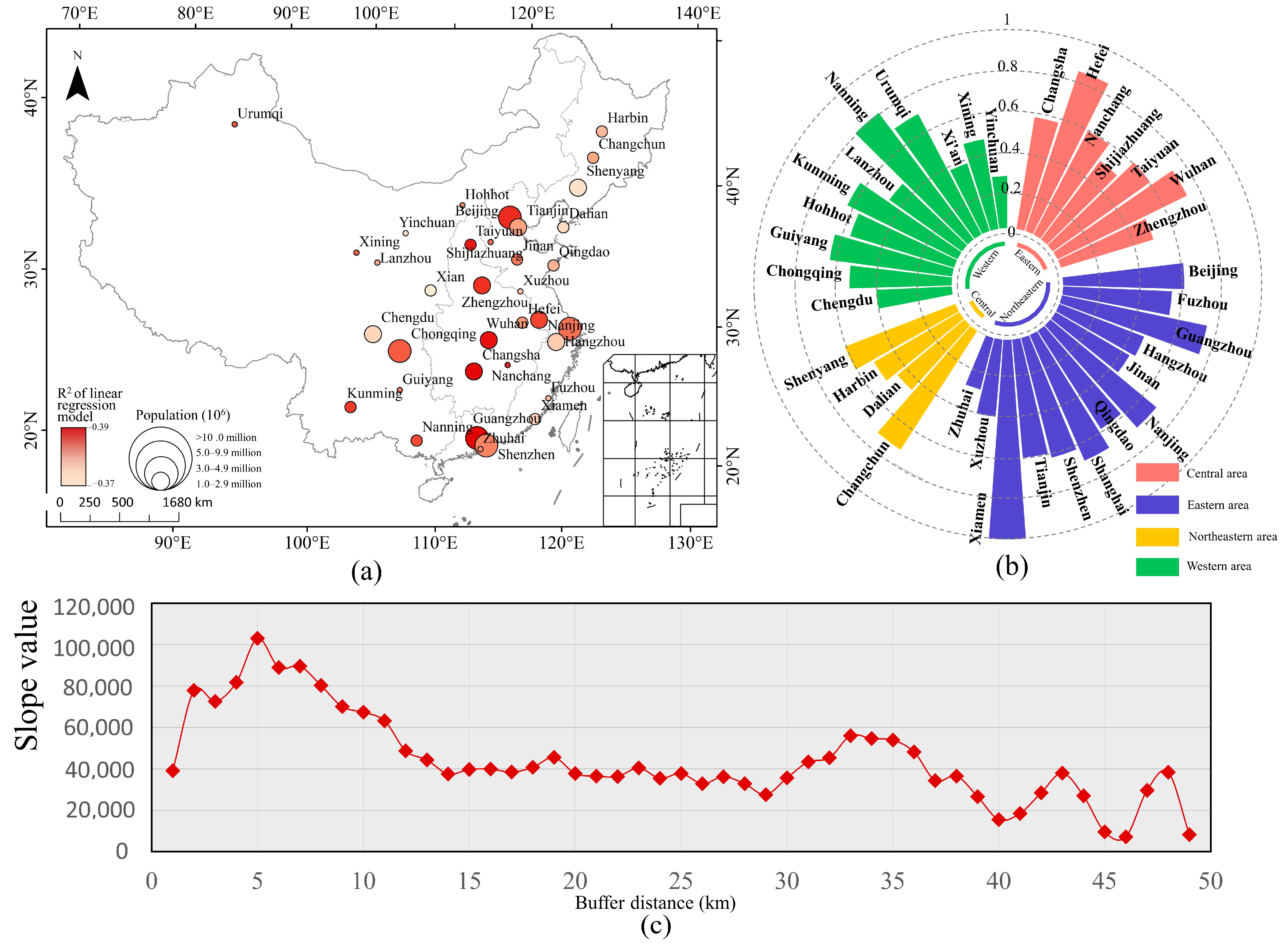
3.1. The Distribution of UBUE

We first validated BVD, UFI, and UBUE using two local urban areas in Beijing. High-resolution satellite imagery and gridded spatial distribution maps of BVD, UFI, and UBUE for the selected areas are presented here. Figure 3a–d and Figure 3e–h correspond to two distinct urban locations. By comparing Figure 3a, Figure 3b and Figure 3c, both building volume and urban function are lowest in the central park area. In contrast, the dense residential area north of the park exhibits high BVD and strong UFI, with moderate UBUE values. Notably, the highest UBUE values appear within the park area itself. This is because, despite the low building volume, the park is with nighttime lighting and urban facilities, indicating high functional efficiency per unit of building. Figure 3e–h represents BVD, UFI, and UBUE in another Beijing subarea, where northern regions show significantly higher BVD and UFI than southern areas. However, southern areas exhibit higher UBUE, likely due to lower building density. Together, these case studies not only validate the reliability of BVD and UFI data against high-resolution satellite imagery but also illustrate the derivation process of UBUE from BVD and UFI.
The UBUE values for the 35 cities are shown in Figure 4a. The most efficient cities were located in the eastern and western areas of China. Chengdu, Shenzhen, and Xi’an had the highest UBUE, indicating that their per unit buildings carried more urban function than those in other cities. In contrast, Zhuhai, Changchun, and Xuzhou were the bottom three cities in the UBUE ranking list. The highest UBUE of the sample cities was 4.3 times greater than the lowest value. The average UBUE was similar across the four regions of China, although it was slightly higher in the cities in the western area, as indicated by the t-test. We further examined the SAMIs of the selected cities (Figure 4b,c). In general, the average SAMI values for 60% of the cities were negative, indicating that the UFI was below the expected value. Shenzhen, Chengdu, and Guiyang had the highest SAMI values, which significantly exceeded the expected value suggested by the regression analysis.
The UBUE and SAMI values of all the buffer areas in the selected cities were examined. These buffer areas were the multiple buffer rings with 1 km intervals. The average UBUE value of the different buffers in the 35 cities displayed a stable declining trend from the urban core areas to the outer areas (Figure 5a). The UBUE of the urban core area remained high within the buffer distance of 10 km. The most intensive UBUE was determined in the 10th buffer, which was 2.3 times higher than the 20th buffer and 8.4 times higher than the 50th buffer (Figure 5b). The accumulated UFI within the buffer distance of 10 km was 59.1%, indicating that more than half of the total urban function of China’s major cities was carried by buildings in the urban core areas. We further examined the buffer areas of each city where the SAMI first fell below 0 along the urban–rural gradient (Figure 5c). Almost all the buffer areas in Shenzhen and Chengdu had positive SAMIs. Shanghai, Guangzhou, and Beijing also had relatively large areas with positive SAMIs. In comparison, only a small fraction of the buffers had a positive SAMI in Yinchuan, Jinan, and Tianjin, indicating that only the very central areas had a UFI that exceeded the expected value.

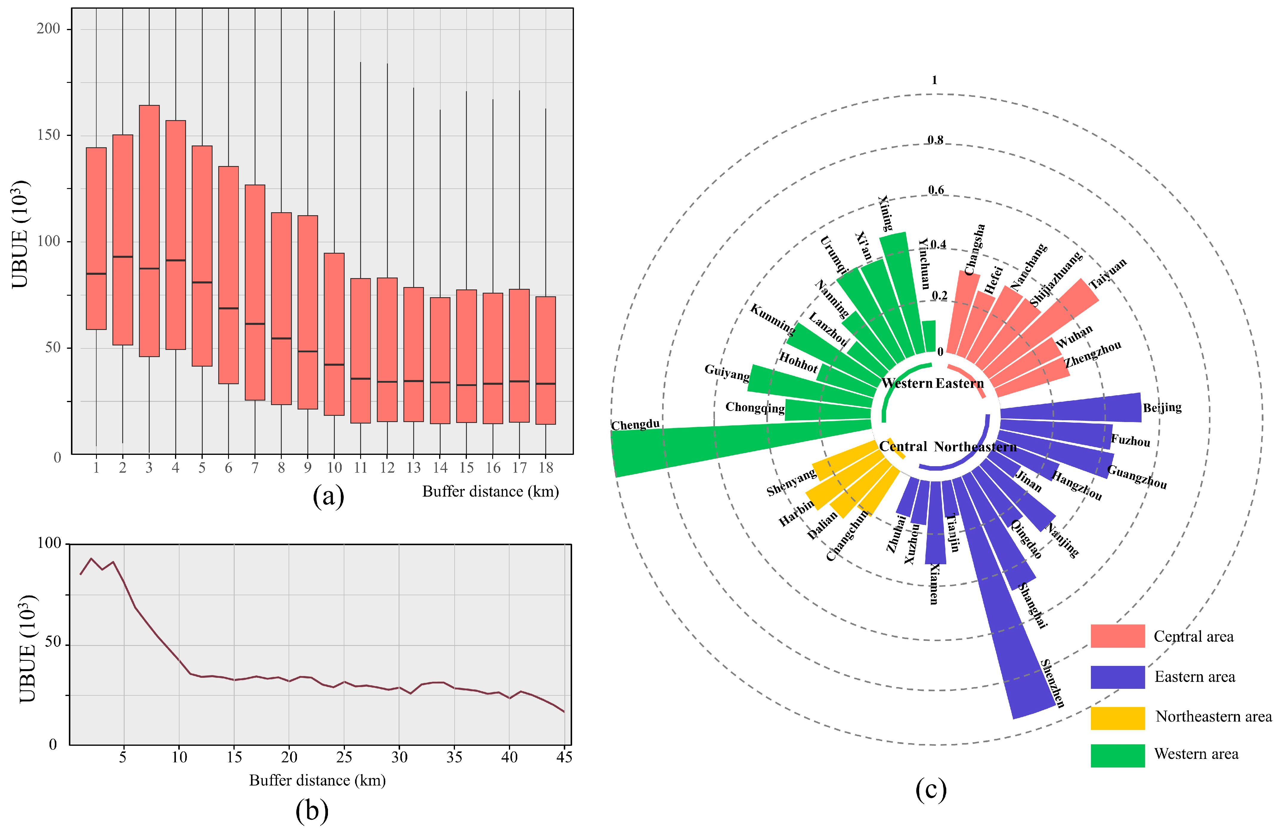
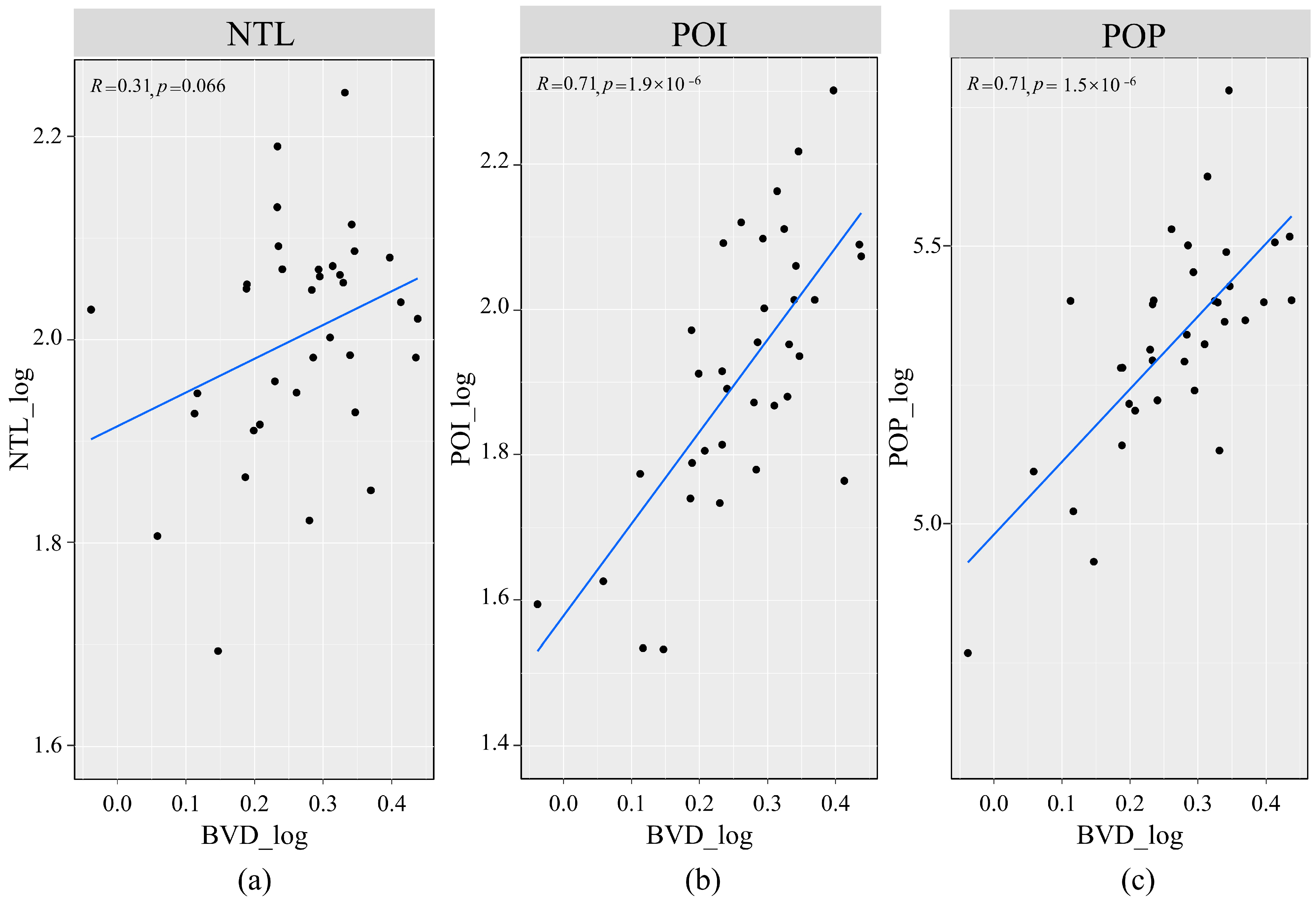
3.2. The Relationship Between UFI and BVD

The relationships between BVD and three selected urban efficiency indicators in the sample cities and grid pixels are shown in Figure 6 and Figure 7. All the urban efficiency indicators significantly increased as the BVD increased. Comparatively, the POI and POP were more closely related to BVD, which was confirmed by the R2 values of their linear regression models. At the grid level, the urban efficiency indicators increased as the BVD increased in all regions. The relationship was more positive in the northeastern area (Figure 7). The slope value of the model for the BVD and NTL relationship in the northeastern area was 1.8 times that of the central area, indicating that an increase in the BVD in the northeastern area would generate 80% more NTL than the equivalent increase in the central area.
The spatial variation of the relationship between UFI and BVD was also examined within different cities and buffer areas using linear regression models. The slope values indicated the newly increased urban functions brought by per unit building volume. These linear regression models varied significantly (Figure 8a,b). The linear regression model regarding UFI and BVD for Xiamen had the highest slope value, which was 3.8 times greater than that of Yinchuan. This result suggested that the same increase in building volume in Xiamen would generate 3.8 times more UFI than in Yinchuan. Cities in the central area had the highest slope value, followed by the eastern, northeastern, and western areas. An increase in building volume in the cities in the central area would generate 19% more UFI than the equivalent increase in building volume in the cities in the western area.
We divided the pixel grids by the buffer distance and constructed linear regression models for each of them. The slope values of these models are presented in Figure 8c, which shows a fluctuating pattern according to the increase in buffer distance. The slope value reached a peak in the buffer area 5 km from the central point of the city, and there was a rapid decline in the buffer rings within the distances from 5 to 15 km. The second peak slope value occurred around a distance of 35 km, which was about half of the first peak value. Besides, the slope values slightly fluctuated between the buffer distances of 15 and 30 km and sharply fluctuated outside the buffer distance of 40 km. These results confirm that intensive construction in the urban core area is more efficient for sustaining UFI.

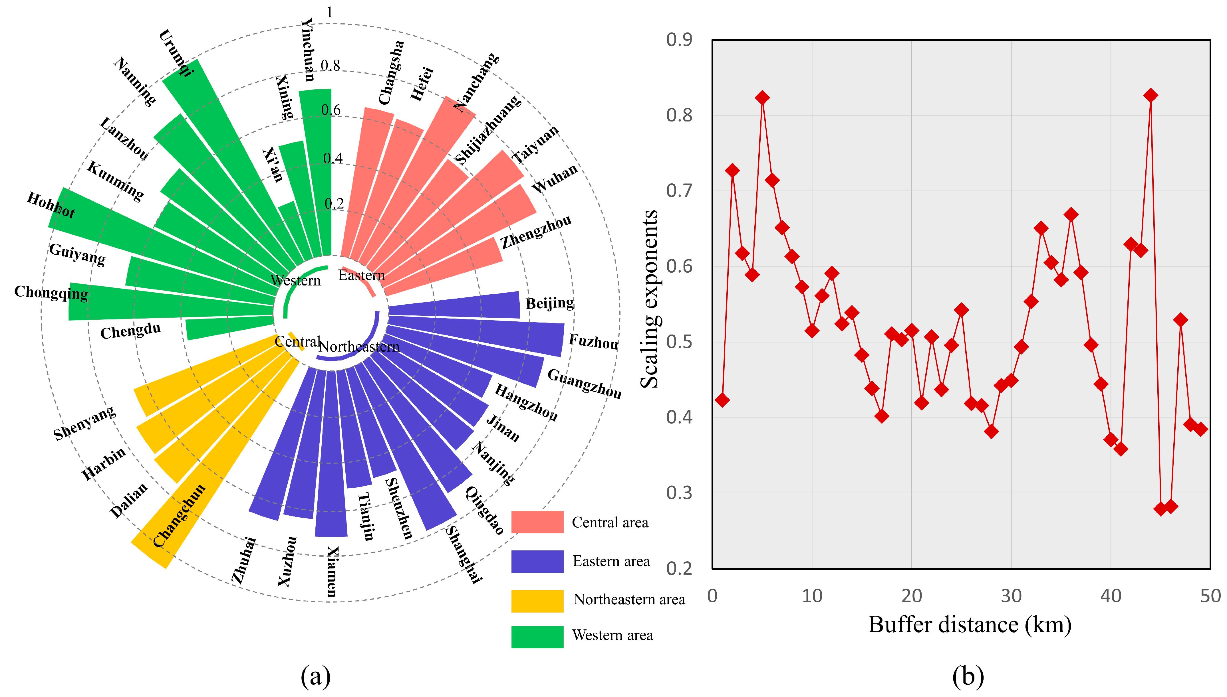
3.3. Spatial Heterogeneity of Scaling Exponents

We further fitted a scaling relationship between BVD and UFI at the national level for 35 cities applying the power function model (Figure 9a). The residuals of the fitted functions in all cities exhibited characteristics consistent with a normal distribution. The national-level scaling exponents varied from 0.26 to 1.07, with a median value of 0.67. Among the 35 cities, only two had a scaling exponent greater than 1, indicating that most cities had a sub-linear relationship between urban function and building volume. The top three cities with the highest scaling exponents were Changchun, Hohhot, and Urumqi. The average scaling exponents of cities in the central, eastern, and western areas were similar and significantly lower than the values for cities in the northeastern area. We further examined the relationship of scaling exponents with GDP and public budget expenditure indicators (Figure 10a). Only the GDP per capita was negatively correlated with the scaling exponent of cities, indicating that the per unit building construction in developing cities would generate relatively more UFI.
The scaling exponents of the different buffer areas are shown in Figure 9b. The pattern of the scaling exponents shows a gradual decline along the urban–rural gradient. The scaling exponents were relatively higher in two buffer rings: within the buffer distance of 10 km and between the buffer distances of 30 to 40 km. An increase in building volume in these areas would achieve a slight decrease in the marginal diminishing effect and, therefore, carry more urban function. Additionally, the scaling exponents fluctuated intensively beyond the buffer distance of 40 km and were stable at a distance of 10 to 30 km.

4. Discussion

4.1. Theoretical Understanding of UBUE Spatial Variation

Although previous studies revealed a close relationship between urban land use intensity and urban functions [31,56], the concept of UBUE has not been further developed due to the lack of precise three-dimensional measurements of urban buildings at a large scale. UBUE accurately reflects the actual fixed asset investment input–output ratio compared with urban land efficiency, which serves as a major indicator of urban fiscal and energy stress caused by excessive real estate development. Our results indicate that urban building use efficiency exhibits significant differences among different cities and different locations within urban areas. This can be explained by the inherent spatial differentiation pattern of human activity intensity, which varies significantly along urban–rural gradients. Such a spatial pattern is in line with the densification of urban centers and the de-densification of surrounding areas, as determined by land rent gradients [57]. Similarly, differences in human activity intensity also exist among different cities at the national scale, which are determined by economic development levels and population density [58]. Our results also suggest that an increase in building volume does not necessarily ensure the desired level of human activity and a vibrant urban environment, which is in line with local investigations conducted in previous studies [21].

4.2. Implication for Land Development Rights at the National Scale

The spatial variation of the relationship between building volume and urban functions provides a new scientific basis for land development rights at the national scale. Existing literature and policies concerning built-up land quota allocations evaluate the need for the quota based on current land use efficiency. The underlying assumption is that the construction of new urban buildings in cities with high land use efficiency would remain efficient over time [59]. However, our results show that in cities with high UBUE, an increase in building volume does not necessarily generate sufficient urban function as expected.
We applied quadrant analysis to investigate the relationship between UBUE and the slope value (Figure 11). The slope value was calculated using linear regression models fitting urban function and building volume at the pixel level in different cities. These cities were divided into four categories according to their current UBUE and the ratios of increase in urban function to increase in building volume. For instance, cities in the IV quadrant had a high current UBUE but a low increase in urban function with increased building volume, which is quantified by the slope value of the linear regression model. Although buildings in these cities currently carry urban function efficiently, further increases in building volume would generate less urban function than equivalent increases in other cities. This finding contrasts with the previous basic notion regarding the inter-regional allocation of new built-up land, which prioritized limited built-up land quotas for cities with high current land use efficiency [60]. Therefore, we suggest that built-up land quota allocation policies at the national scale should consider differences in the urban function capacities of newly increased built-up land.
In addition, the significant negative correlation between GDP per unit land area and scaling exponents indicates that in more economically developed cities, the marginal diminishing effects of increasing BVD on UFI are more pronounced. Therefore, enhancing building volume to boost functionality represents a strategic option for less-developed cities, particularly those in the northeastern and western regions. Northeastern cities exhibit the lowest UBUE among all regions, though the slope of the UBUE–BVD regression model is not the lowest. This can be attributed to the early development of northeastern cities, which led to relatively high construction intensity in built-up areas. In recent years, however, these cities have experienced significant population outflows, resulting in widespread building vacancies and, consequently, low UBUE values. Nevertheless, the relatively high slope of the UBUE–BVD relationship in these cities suggests strong sensitivity of UFI to BVD changes, implying that high-density zones do not suffer severe underutilization. This indicates that northeastern cities retain the capacity to attract rural populations from surrounding areas, albeit less effectively than central and eastern cities. In contrast, western cities currently show higher UBUE but the lowest UBUE–BVD slopes among all regions. The elevated UBUE in western cities may arise from geographic constraints limiting built-up area expansion, thereby concentrating urban functions within a smaller building volume and enhancing current utilization efficiency. However, the low slope value suggests limited additional urban functionality from increased development intensity, indicating constrained growth potential for urban functions. In summary, while western cities exhibit higher current UBUE, northeastern cities demonstrate greater marginal value in additional building development for functional growth.

4.3. Urban Growth Strategies at the Urban Scale

With the continuous population expansion in large cities, urban growth through new building construction is required to accommodate increases in urban functions. Consequently, a rational spatial allocation of these new buildings, aiming at achieving efficient building use efficiency becomes a vital decision for urban planners. Our study indicated that the current UBUE displayed a significant decreasing trend along the urban–rural gradient, suggesting that buildings located in the city center have a higher functional carrying efficiency. Similarly, the BVD−UFI slope value also generally decreased along the urban–rural gradient. This implies that an increase in building volume in the urban core would be conducive to improving UBUE because each unit increase in building volume in the city center will result in greater urban function. This finding demonstrates the potential for improvements in building use efficiency in the core areas of developed cities [22], and also confirms the contribution of urban renewal activities to urban vitality [51]. Urban renewal activities that aim to promote UBUE in the urban core area will help avoid losing neighborhood vitality during rapid urbanization [61,62].
The statistical results also indicated that, in most cities, the increased urban function generated by new buildings showed marginal diminishing effects. In other words, new developments in low-intensity areas tended to contribute more significantly to the enhancement of urban function. In contrast, additional construction in high-intensity development zones yielded markedly lower marginal gains in urban function. A possible explanation is that the supporting capacity of infrastructure and service facilities in these areas may have been fully used. This finding suggests that a more balanced development strategy across the entire urban area is more effective in improving the utilization efficiency of new buildings compared to a polarized development strategy focused on specific zones. Therefore, underutilized, low-intensity development zones should be prioritized for redevelopment to improve overall building utilization efficiency. These results will enable urban land use policymakers to make more informed urban development strategies.

5. Conclusions

This study proposes an urban building use efficiency evaluation method and further innovatively examines the efficiency of urban building use from the dual perspective of stock and increment. Taking 35 of the major cities in China as samples, we uncovered disparities in the relationship between urban function and building volume at both national and city scales. The main findings can be summarized as follows: First, the UFIs carried by a unit building volume in different regions were significantly different. Among the 35 cities, the maximum disparity in UBUE between different cities was 4.3 times. At the urban scale, the UBUE gradually decreased along the urban–rural gradient. Second, the new urban function generated by an increase in building volume was also spatially heterogeneous, although the disparity among cities was not as significant as that for UBUE. Third, almost all of the selected cities exhibited a marginal diminishing effect in the relationship between building volume and urban functions. Moreover, this marginal diminishing effect was more pronounced in economically developed cities.
This study made two explicit contributions to the field of urban planning and development. First, by considering three-dimensional buildings as the measurement object for the utility efficiency of urban areas, we provided a more precise evaluation of how the urban built environment carries urban function than the existing research. Previous studies primarily focused on land use efficiency measured in two dimensions, neglecting the decisive role of the three-dimensional urban morphology in actual fixed asset investments, long-term energy consumption, and carbon emissions. The accurate depiction of UBUE in this study revealed building resource consumption waste and fiscal risk due to excessive urban building construction. On this account, the measurement of UBUE provides a scientific basis for three-dimensional urban land use regulation. Second, the dual examination of UBUE from both stock and increment perspectives enabled new insights into land use policy, including the allocation policy for land development rights and urban growth management. Traditionally, historic urban land use efficiency has been used as a key criterion for the allocation of land development rights, neglecting the differences in the building use efficiency of increased building volumes. We considered that allocation policy for land development rights should be more forward-looking, relying not only on historic utility efficiency of the urban area, but also on the urban function brought by new buildings, as well as the diminishing marginal effects of building volume increases on urban functions. Also, we suggest that building renewal aimed at improving utility efficiency in urban core areas should be carried out. The increase of building volume in such areas would achieve more urban function, especially for areas with current low density.
The limitations of the study were as follows. First, the mechanisms driving regional UBUE variation require further exploration. Although spatial variations in UBUE at both national and urban scales were identified, the pathways through which socioeconomic factors influence UBUE remain unclear. Establishing a robust theoretical foundation for linking UBUE to socioeconomic development indicators is necessary. Second, the relationship between building volume increments and urban function growth requires simulation via a more comprehensive quantitative model. The underlying factors shaping the relationship between the two remain insufficiently explored, constraining the development of more targeted and effective urban planning interventions. Third, high-density development may impose significant pressure on transportation systems and various public service facilities, which in turn could hinder the efficient functioning of urban systems. This feedback relationship, however, has not been sufficiently addressed in the current manuscript. Fourth, the three-dimensional building data utilized in this study enables the calculation of building volume but does not provide information on floor area. Floor area is generally considered a more suitable indicator for assessing the relationship between urban morphology and urban function, given its verifiability, widespread use in official sectoral statistics, and direct relevance to land use regulation.

Author Contributions

Conceptualization, T.H. and Y.L.; methodology, T.H.; software, Y.L.; validation, T.H., Y.L. and S.C.; formal analysis, M.Z.; investigation, Y.L.; resources, S.C.; data curation, A.G.; writing—original draft preparation, T.H. and Y.L.; writing—review and editing, Y.L. and S.C.; visualization, B.L.; supervision, S.C.; project administration, T.H.; funding acquisition, Y.L. and A.G. All authors have read and agreed to the published version of the manuscript.

Funding

This work was supported by the National Natural Science Foundation of China [grant numbers 52208088, 42201307, 52278062].

Data Availability Statement

Data will be made available on request.

Conflicts of Interest

The authors declare no conflicts of interest.

Abbreviations

The following abbreviations are used in the manuscript:
UBUEUrban building use efficiency
BVDBuilding volume density
UFIUrban function intensity
POIPoint of interest
NTLNighttime light

References

  1. Zhao, P. Managing Urban Growth in a Transforming China: Evidence from Beijing. Land. Use Policy 2011, 28, 96–109. [Google Scholar] [CrossRef]
  2. Li, J.; Li, C.; Zhu, F.; Song, C.; Wu, J. Spatiotemporal Pattern of Urbanization in Shanghai, China between 1989 and 2005. Landsc. Ecol. 2013, 28, 1545–1565. [Google Scholar] [CrossRef]
  3. Huq, S.; Kovats, S.; Reid, H.; Satterthwaite, D. Reducing Risks to Cities from Disasters and Climate Change. Environ. Urban. 2007, 19, 3–15. [Google Scholar] [CrossRef]
  4. Liu, Z.; He, C.; Zhou, Y.; Wu, J. How Much of the World’s Land Has Been Urbanized, Really? A Hierarchical Framework for Avoiding Confusion. Landsc. Ecol. 2014, 29, 763–771. [Google Scholar] [CrossRef]
  5. Klotz, M.; Kemper, T.; Geiß, C.; Esch, T.; Taubenböck, H. How Good Is the Map? A Multi-Scale Cross-Comparison Framework for Global Settlement Layers: Evidence from Central Europe. Remote Sens. Env. 2016, 178, 191–212. [Google Scholar] [CrossRef]
  6. Laroche, P.C.S.J.; Schulp, C.J.E.; Kastner, T.; Verburg, P.H. Telecoupled Environmental Impacts of Current and Alternative Western Diets. Glob. Environ. Change 2020, 62, 102066. [Google Scholar] [CrossRef]
  7. Gao, J.; O’Neill, B.C. Mapping Global Urban Land for the 21st Century with Data-Driven Simulations and Shared Socioeconomic Pathways. Nat. Commun. 2020, 11, 2302. [Google Scholar] [CrossRef] [PubMed]
  8. Assembly, G. Resolution Adopted by the General Assembly on 11 September 2015; United Nations: New York, NY, USA, 2015. [Google Scholar]
  9. Gao, J.; Chen, W.; Yuan, F. Spatial Restructuring and the Logic of Industrial Land Redevelopment in Urban China: I. Theoretical Considerations. Land. Use Policy 2017, 68, 604–613. [Google Scholar] [CrossRef]
  10. Lin, J.; Wan, H.; Cui, Y. Analyzing the Spatial Factors Related to the Distributions of Building Heights in Urban Areas: A Comparative Case Study in Guangzhou and Shenzhen. Sustain. Cities Soc. 2020, 52, 101854. [Google Scholar] [CrossRef]
  11. Mahtta, R.; Mahendra, A.; Seto, K.C. Building up or Spreading out? Typologies of Urban Growth across 478 Cities of 1 Million+. Environ. Res. Lett. 2019, 14, 124077. [Google Scholar] [CrossRef]
  12. Zheng, Z.; Zhou, W.; Wang, J.; Hu, X.; Qian, Y. Sixty-Year Changes in Residential Landscapes in Beijing: A Perspective from Both the Horizontal (2D) and Vertical (3D) Dimensions. Remote Sens. 2017, 9, 992. [Google Scholar] [CrossRef]
  13. Shen, L.; Shu, T.; Liao, X.; Yang, N.; Ren, Y.; Zhu, M.; Cheng, G.; Wang, J. A New Method to Evaluate Urban Resources Environment Carrying Capacity from the Load-and-Carrier Perspective. Resour. Conserv. Recycl. 2020, 154, 104616. [Google Scholar] [CrossRef]
  14. Huang, Z.; He, C.; Zhu, S. Do China’s Economic Development Zones Improve Land Use Efficiency? The Effects of Selection, Factor Accumulation and Agglomeration. Landsc. Urban. Plan. 2017, 162, 145–156. [Google Scholar] [CrossRef]
  15. Du, J.; Thill, J.-C.; Peiser, R.B. Land Pricing and Its Impact on Land Use Efficiency in Post-Land-Reform China: A Case Study of Beijing. Cities 2016, 50, 68–74. [Google Scholar] [CrossRef]
  16. Huang, Z.; Bao, Y.; Mao, R.; Wang, H.; Yin, G.; Wan, L.; Qi, H.; Li, Q.; Tang, H.; Liu, Q. Big Geodata Reveals Spatial Patterns of Built Environment Stocks across and within Cities in China. Engineering 2024, 34, 143–153. [Google Scholar] [CrossRef]
  17. Banister, D.; Watson, S.; Wood, C. Sustainable Cities: Transport, Energy, and Urban Form. Environ. Plann B Plann Des. 1997, 24, 125–143. [Google Scholar] [CrossRef]
  18. Katsavounidou, G. Life between Buildings: Using Public Space: The History of Jan Gehl’s Book and the Legacy of Its Philosophy for Designing Cities at Human Scale. In The Future of Central Urban Areas: Sustainable Planning and Design Perspectives from Thessaloniki, Greece; Institutionelles Repositorium der Leibniz Universität Hannover: Hanover, Germany, 2023; pp. 21–37. [Google Scholar]
  19. Jane, J. The Life and Death of Great American Cities; Random House: New York, NY, USA, 1961. [Google Scholar]
  20. Zhong, C.; Schläpfer, M.; Müller Arisona, S.; Batty, M.; Ratti, C.; Schmitt, G. Revealing Centrality in the Spatial Structure of Cities from Human Activity Patterns. Urban. Stud. 2017, 54, 437–455. [Google Scholar] [CrossRef]
  21. Xia, C.; Yeh, A.G.; Zhang, A. Analyzing Spatial Relationships between Urban Land Use Intensity and Urban Vitality at Street Block Level: A Case Study of Five Chinese Megacities. Landsc. Urban. Plan. 2020, 193, 103669. [Google Scholar] [CrossRef]
  22. Ruan, L.; He, T.; Xiao, W.; Chen, W.; Lu, D.; Liu, S. Measuring the Coupling of Built-up Land Intensity and Use Efficiency: An Example of the Yangtze River Delta Urban Agglomeration. Sustain Cities Soc. 2022, 87, 104224. [Google Scholar] [CrossRef]
  23. Lee, J.H.; Lim, S. The Selection of Compact City Policy Instruments and Their Effects on Energy Consumption and Greenhouse Gas Emissions in the Transportation Sector: The Case of South Korea. Sustain. Cities Soc. 2018, 37, 116–124. [Google Scholar] [CrossRef]
  24. Kremer, P.; Haase, A.; Haase, D. The Future of Urban Sustainability: Smart, Efficient, Green or Just? Introduction to the Special Issue. Sustain. Cities Soc. 2019, 51, 101761. [Google Scholar] [CrossRef]
  25. Burger, M.; Meijers, E. Form Follows Function? Linking Morphological and Functional Polycentricity. Urban. Stud. 2012, 49, 1127–1149. [Google Scholar] [CrossRef]
  26. Chen, Z.; Tang, J.; Wan, J.; Chen, Y. Promotion Incentives for Local Officials and the Expansion of Urban Construction Land in China: Using the Yangtze River Delta as a Case Study. Land. Use Policy 2017, 63, 214–225. [Google Scholar] [CrossRef]
  27. Chen, K. Ghost Cities of China. The Story of Cities Without People in the World’s Most Populated Country. Eur.-Asia Stud. 2017, 69, 998–999. [Google Scholar] [CrossRef]
  28. Lin, J.; Lu, S.; He, X.; Wang, F. Analyzing the Impact of Three-Dimensional Building Structure on CO2 Emissions Based on Random Forest Regression. Energy 2021, 236, 121502. [Google Scholar] [CrossRef]
  29. Zitti, M.; Ferrara, C.; Perini, L.; Carlucci, M.; Salvati, L. Long-Term Urban Growth and Land Use Efficiency in Southern Europe: Implications for Sustainable Land Management. Sustainability 2015, 7, 3359–3385. [Google Scholar] [CrossRef]
  30. Zhang, L.; Zhang, L.; Xu, Y.; Zhou, P.; Yeh, C.-H. Evaluating Urban Land Use Efficiency with Interacting Criteria: An Empirical Study of Cities in Jiangsu China. Land. Use Policy 2020, 90, 104292. [Google Scholar] [CrossRef]
  31. Wu, C.; Wei, Y.D.; Huang, X.; Chen, B. Economic Transition, Spatial Development and Urban Land Use Efficiency in the Yangtze River Delta, China. Habitat. Int. 2017, 63, 67–78. [Google Scholar] [CrossRef]
  32. Zhang, W.; Wang, B.; Wang, J.; Wu, Q.; Wei, Y.D. How Does Industrial Agglomeration Affect Urban Land Use Efficiency? A Spatial Analysis of Chinese Cities. Land. Use Policy 2022, 119, 106178. [Google Scholar] [CrossRef]
  33. Cui, X.; Wang, X. Urban Land Use Change and Its Effect on Social Metabolism: An Empirical Study in Shanghai. Habitat. Int. 2015, 49, 251–259. [Google Scholar] [CrossRef]
  34. Ye, Y.; Li, D.; Liu, X. How Block Density and Typology Affect Urban Vitality: An Exploratory Analysis in Shenzhen, China. Urban. Geogr. 2018, 39, 631–652. [Google Scholar] [CrossRef]
  35. Moroni, S. Urban Density after Jane Jacobs: The Crucial Role of Diversity and Emergence. City Territ. Archit. 2016, 3, 1–8. [Google Scholar] [CrossRef]
  36. Wang, Y.; Yue, X.; Li, C.; Wang, M.; Zhang, H.; Su, Y. Relationship between Urban Three-Dimensional Spatial Structure and Population Distribution: A Case Study of Kunming’s Main Urban District, China. Remote Sens. 2022, 14, 3757. [Google Scholar] [CrossRef]
  37. Pickett, S.T.A.; Cadenasso, M.L.; Childers, D.L.; Mcdonnell, M.J.; Zhou, W. Evolution and Future of Urban Ecological Science: Ecology in, of, and for the City. Ecosyst. Health Sustain. 2016, 2, e01229. [Google Scholar] [CrossRef]
  38. Xu, G.; Xiu, T.; Li, X.; Liang, X.; Jiao, L. Lockdown Induced Night-Time Light Dynamics during the COVID-19 Epidemic in Global Megacities. Int. J. Appl. Earth Obs. Geoinf. 2021, 102, 102421. [Google Scholar] [CrossRef]
  39. Wu, B.; Yang, C.; Chen, Z.; Wu, Q.; Yu, S.; Wang, C.; Li, Q.; Wu, J.; Yu, B. The Relationship between Urban 2-D/3-D Landscape Pattern and Nighttime Light Intensity. IEEE J. Sel. Top. Appl. Earth Obs. Remote Sens. 2021, 15, 478–489. [Google Scholar] [CrossRef]
  40. Kuang, W.; Liu, J.; Dong, J.; Chi, W.; Zhang, C. The Rapid and Massive Urban and Industrial Land Expansions in China between 1990 and 2010: A CLUD-Based Analysis of Their Trajectories, Patterns, and Drivers. Landsc. Urban. Plan. 2016, 145, 21–33. [Google Scholar] [CrossRef]
  41. Zhu, Z.; Zhou, Y.; Seto, K.C.; Stokes, E.C.; Deng, C.; Pickett, S.T.A.; Taubenböck, H. Understanding an Urbanizing Planet: Strategic Directions for Remote Sensing. Remote Sens. Environ. 2019, 228, 164–182. [Google Scholar] [CrossRef]
  42. Li, K.; Li, Y.; Yang, X.; Liu, X.; Huang, Q. Comparing the Three-Dimensional Morphologies of Urban Buildings along the Urban-Rural Gradients of 91 Cities in China. Cities 2023, 133, 104123. [Google Scholar] [CrossRef]
  43. Gong, P.; Li, X.; Wang, J.; Bai, Y.; Chen, B.; Hu, T.; Liu, X.; Xu, B.; Yang, J.; Zhang, W. Annual Maps of Global Artificial Impervious Area (GAIA) between 1985 and 2018. Remote Sens. Environ. 2020, 236, 111510. [Google Scholar] [CrossRef]
  44. Wu, W.-B.; Ma, J.; Banzhaf, E.; Meadows, M.E.; Yu, Z.-W.; Guo, F.-X.; Sengupta, D.; Cai, X.-X.; Zhao, B. A First Chinese Building Height Estimate at 10 m Resolution (CNBH-10 m) Using Multi-Source Earth Observations and Machine Learning. Remote Sens. Environ. 2023, 291, 113578. [Google Scholar] [CrossRef]
  45. Wu, L.; Gong, C.; Yan, X. Taylor’s Power Law and Its Decomposition in Urban Facilities. R. Soc. Open Sci. 2019, 6, 180770. [Google Scholar] [CrossRef]
  46. Xu, R.; Yue, W.; Wei, F.; Yang, G.; He, T.; Pan, K. Density Pattern of Functional Facilities and Its Responses to Urban Development, Especially in Polycentric Cities. Sustain. Cities Soc. 2021, 76, 103526. [Google Scholar] [CrossRef]
  47. Li, X.; Gong, P.; Zhou, Y.; Wang, J.; Bai, Y.; Chen, B.; Hu, T.; Xiao, Y.; Xu, B.; Yang, J. Mapping Global Urban Boundaries from the Global Artificial Impervious Area (GAIA) Data. Environ. Res. Lett. 2020, 15, 94044. [Google Scholar] [CrossRef]
  48. Tatem, A.J. WorldPop, Open Data for Spatial Demography. Sci. Data 2017, 4, 170004. [Google Scholar] [CrossRef] [PubMed]
  49. Chen, Z.; Wei, Y.; Shi, K.; Zhao, Z.; Wang, C.; Wu, B.; Qiu, B.; Yu, B. The Potential of Nighttime Light Remote Sensing Data to Evaluate the Development of Digital Economy: A Case Study of China at the City Level. Comput. Environ. Urban. Syst. 2022, 92, 101749. [Google Scholar] [CrossRef]
  50. Jiao, L. Urban Land Density Function: A New Method to Characterize Urban Expansion. Landsc. Urban. Plan. 2015, 139, 26–39. [Google Scholar] [CrossRef]
  51. Tan, X.; Huang, B.; Batty, M.; Li, W.; Wang, Q.R.; Zhou, Y.; Gong, P. The Spatiotemporal Scaling Laws of Urban Population Dynamics. Nat. Commun. 2025, 16, 2881. [Google Scholar] [CrossRef]
  52. Barthelemy, M. The Statistical Physics of Cities. Nat. Rev. Phys. 2019, 1, 406–415. [Google Scholar] [CrossRef]
  53. Bettencourt, L.M.A. The Origins of Scaling in Cities. Science (1979) 2013, 340, 1438–1441. [Google Scholar] [CrossRef]
  54. Xu, G.; Zhu, M.; Chen, B.; Salem, M.; Xu, Z.; Li, X.; Jiao, L.; Gong, P. Settlement Scaling Law Reveals Population-Land Tensions in 7000 + African Urban Agglomerations. Habitat. Int. 2023, 142, 102954. [Google Scholar] [CrossRef]
  55. Lobo, J.; Bettencourt, L.M.A.; Smith, M.E.; Ortman, S. Settlement Scaling Theory: Bridging the Study of Ancient and Contemporary Urban Systems. Urban. Stud. 2020, 57, 731–747. [Google Scholar] [CrossRef]
  56. Chen, Y.; Chen, Z.; Xu, G.; Tian, Z. Built-up Land Efficiency in Urban China: Insights from the General Land Use Plan (2006–2020). Habitat. Int. 2016, 51, 31–38. [Google Scholar] [CrossRef]
  57. Alonso, W. Location and Land Use: Toward a General Theory of Land Rent; Harvard University Press: Cambridge, MA, USA, 1964; ISBN 0674729560. [Google Scholar]
  58. Li, M.; Verburg, P.H.; van Vliet, J. Global Trends and Local Variations in Land Take per Person. Landsc. Urban. Plan. 2022, 218, 104308. [Google Scholar] [CrossRef]
  59. Yan, S.; Peng, J.; Wu, Q. Exploring the Non-Linear Effects of City Size on Urban Industrial Land Use Efficiency: A Spatial Econometric Analysis of Cities in Eastern China. Land. Use Policy 2020, 99, 104944. [Google Scholar] [CrossRef]
  60. He, T.; Lu, Y.; Yue, W.; Xiao, W.; Shen, X.; Shan, Z. A New Approach to Peri-Urban Area Land Use Efficiency Identification Using Multi-Source Datasets: A Case Study in 36 Chinese Metropolitan Areas. Appl. Geogr. 2023, 150, 102826. [Google Scholar] [CrossRef]
  61. Hosseini, A.; Pourahmad, A.; Taeeb, A.; Amini, M.; Behvandi, S. Renewal Strategies and Neighborhood Participation on Urban Blight. Int. J. Sustain. Built Environ. 2017, 6, 113–121. [Google Scholar] [CrossRef]
  62. Ahmed, S.; Bramley, G. How Will Dhaka Grow Spatially in Future?-Modelling Its Urban Growth with a near-Future Planning Scenario Perspective. Int. J. Sustain. Built Environ. 2015, 4, 359–377. [Google Scholar] [CrossRef]
Figure 1. Regional zoning of the selected cities. The eastern, central, western, and northeastern areas are distinguished by different colors. The size of the circles indicates the population of the cities, which were classified into type II big cities (1.0–2.9 million people), type I big cities (3.0–4.9 million people), supercities (5.0–9.9 million people), and megacities (>10.0 million people) according to the official standards used in China.
Buildings 15 01803 g001
Figure 2. Illustration of building volume density calculation (BVD). Building volume data were retrieved from the dataset of CNBH-10 m. The impervious area within the 1 km2 sample grid is identified for BVD calculation (Equation (1)).
Buildings 15 01803 g002
Figure 3. Validation of BVD, UFI, and UBUE using two local urban areas in Beijing. Panels (ad) show the high-resolution image, BVD pattern, UFI pattern, and UBUE pattern for case 1, respectively. Panels (eh) depict the corresponding high-resolution image, BVD pattern, UFI pattern, and UBUE pattern for case 2.
Buildings 15 01803 g003
Figure 4. The urban building use efficiency (UBUE) and scale-adjusted metropolitan indicator (SAMI) in different cities in China. (a) The UBUE of all 1 km2 sample grids within the urban areas of the 35 cities. The error bars represent the mean and 95% confidence intervals of UBUE values. The solid circles indicate the mean UBUE values for each city. (b,c) Indicate the SAMI value of the cities. The colors of the circles in (c) indicate whether the SAMI is more or less than 0, which determines whether the urban function is higher than the expected value. The vertical axis displays the SAMI values for each city, and the size of each circle reflects the corresponding UBUE value.
Buildings 15 01803 g004
Figure 5. (a) The urban building use efficiency (UBUE) in different buffer areas and (b) the normalized buffer distance at which the SAMI first fell to 0 along the urban–rural gradient. (a) The UBUE of all the sample grids in different buffer areas according to their distance to the urban center. The box displays the median, upper quartile, and lower quartile of the data. (a) The UBUE variation along the urban–rural gradient. (c) The buffer distance at which the SAMI first fell to 0 along the urban–rural gradient. Because the sizes of urban areas differed, the buffer area distances were normalized by the maximum buffer distances of the relevant urban area. The lengths of the bars indicate the proportion of the buffer area that had a positive SAMI value.
Buildings 15 01803 g005
Figure 6. Scatter plots of the relationship between building volume density (BVD) and three urban function indicators of the 35 cities. (a) The relationship between BVD and nighttime lights (NTL) intensity. (b) The relationship between BVD and point of interest (POI) density. (c) The relationship between BVD and population (POP) density.
Buildings 15 01803 g006
Figure 7. Scatter plots of the relationship between building volume density (BVD) and three urban function indicators of the sample grids. (a) The relationship between BVD and nighttime lights (NTL) intensity. (b) The relationship between BVD and point of interest (POI) density. (c) The relationship between BVD and population (POP) density.
Buildings 15 01803 g007
Figure 8. The slope values of the linear regression models fitting the relationship between building volume density (BVD) and urban function intensity (UFI). (a,b) Present the R2 and slope values of the linear regression models, respectively. The linear regression models were individually constructed within urban areas by applying the 1 km2 grids. (c) Presents the slope values of the linear regression models constructed in different buffer areas.
Buildings 15 01803 g008
Figure 9. Scaling exponents of 35 cities and different buffer areas. (a) The scaling exponents of 35 cities, as indicated by the length of the bars. Cities in different regions are shown in different colors. (b) The variation of the average scaling exponents along the urban–rural gradient.
Buildings 15 01803 g009
Figure 10. Scatter plots of the selected cities showing the relationship between scaling exponents and socioeconomic indicators. The Y-axis indicates the value of scaling exponents. The X-axis indicates (a) the value of GDP per built-up land, (b) GDP per capita, (c) public budget expenditure per built-up land, and (d) public budget expenditure per capita. The R and p values of the linear regression models are also shown.
Buildings 15 01803 g010
Figure 11. Urban building use efficiency (UBUE) and slope value of sample cities. The classification into four quadrants is based on the median values of the two indicators across all sampled cities. The slope values are retrieved from the linear regression models fitting urban function intensity (UFI) and building volume density (BVD) in different cities. The dotted red lines divide the sample plots into four quadrants according to the median values of UBUE and slope values.
Buildings 15 01803 g011
Table 1. Overview of Datasets Employed in the Study.
DescriptionTimeSpatial ResolutionReference and Sources
Urban area boundary201830 m[47]
Building volume202010 m[44]
Built-up land201830 m[43]
Population data2020100 m[48]
Nighttime light data2020500 m[49]
Point of interest2018-[46]
GDP2017-Ministry of Housing and Urban–Rural Development of the People’s Republic of China
Public budget expenditure2017-Ministry of Housing and Urban–Rural Development of the People’s Republic of China
Disclaimer/Publisher’s Note: The statements, opinions and data contained in all publications are solely those of the individual author(s) and contributor(s) and not of MDPI and/or the editor(s). MDPI and/or the editor(s) disclaim responsibility for any injury to people or property resulting from any ideas, methods, instructions or products referred to in the content.

