1. Introduction
The global demand for climate change mitigation has driven nations worldwide to establish ambitious carbon neutrality commitments. In this context, China’s building sector emerges as a critical energy consumer, with recent data indicating an annual energy use figure exceeding 1 Gtce (gigaton of coal equivalent), representing nearly one-quarter of national energy consumption. Notably, space heating in northern urban areas contributes over one-fifth of the total building-related energy demand [
1]. These consumption patterns present significant challenges to China’s dual goals of reaching peak carbon emissions before 2030 and achieving carbon neutrality by 2060. As a result, the decarbonization of space-heating systems has become a critical priority within the nation’s broader energy transition strategy.
Among renewable alternatives, geothermal energy has emerged as a sustainable solution for space heating and cooling in buildings because of its abundant availability and high efficiency. Based on the extraction depth, geothermal energy can be categorized into shallow geothermal energy (0–200 m deep) and medium-depth geothermal energy (2000–3500 m deep). In order to use geothermal energy more efficiently, it is critical to establish accurate and effective ground heat exchanger models.
As for the shallow geothermal energy applications, researchers have developed a variety of numerical and analytical solution models to analyze the heat transfer characteristics of ground heat exchangers. A numerical simulation is based on employing discretized numerical calculations to solve a problem. The finite volume method (FVM) [
2], finite element method (FEM) [
3], and finite difference method (FDM) [
4] are mainly used to analyze the heat transfer of underground temperature fields. On the other hand, Kelvein [
5] proposed a linear heat source theory model, which laid the foundations for heat transfer analysis in ground heat exchangers. Subsequently, Carslaw and Jaeger [
6] introduced an infinite-length cylindrical heat source model, simplifying the structure within the borehole to an infinitely long linear or cylindrical heat source distributed along the axis. Philippe [
7] further developed a three-dimensional transient far-field boundary heat transfer model, constructed based on the principle of energy balance. As research continues to deepen, theoretical models have been further optimized and refined. For example, Bandos [
8] proposed a three-dimensional finite line source model for borehole heat exchangers (BHEs), which can be used for the design of complex borehole structures. Jia [
9] built an infinite-line source model (ILSM), considering the non-uniformity of specific heat flux along the vertical direction of the borehole wall, and developed an enhanced variable-heat-flux density model using the superposition method.
However, shallow geothermal energy is typically utilized via heat pump technology, and it is well-suited to buildings with relatively balanced heating and cooling loads due to its character of relatively low energy density [
10,
11]. In comparison, medium-depth geothermal systems offer greater energy quality and storage capacity, making them particularly suitable for heating-dominated buildings in northern areas. While conventional U-tube ground heat exchangers (GHEs) are widely employed in shallow geothermal systems, coaxial GHEs are often preferred in medium-depth geothermal systems because of their superior structural stability and enhanced heat transfer performance in deep boreholes exceeding 2000 m [
12].
Over the past decade, medium-depth ground heat exchangers (MDGHEs) have emerged as a transformative geothermal technology in China, undergoing significant advancements in both practical applications and theoretical research. Deng [
13] demonstrated that ground-source heat pump (GSHP) systems incorporating MDGHEs achieved significantly better thermal performance than conventional shallow geothermal systems. Under continuous 48 h operational testing, the system exhibited heat extraction rates per unit borehole length that were 1.5–3.6 times higher than the shallow counterparts. To enhance the performance of MDGHEs, Jiankai Dong [
14] reviewed the effects of multiple factors on the thermal performance of deep-borehole heat exchangers, aiming to guide the design and use of MDGHEs. The results of their study demonstrate that there is a strong positive correlation between inlet and outlet temperatures in MDGHEs. Under high-inlet-temperature conditions (23 °C), these systems consistently deliver elevated outlet temperatures (35 °C), making direct heating possible. Compared to indirect heating systems using medium-depth GSHPs, the direct utilization of circulating fluid from MDGHEs can significantly improve operational efficiency by eliminating the need to activate the heat pump when the fluid temperature is sufficiently high, such as over 30 °C. The direct utilization of MDGHEs for heating purposes has been successful in several developed countries. As shown in
Table 1, critical operational parameters, such as the ground temperatures at the bottom of the borehole and the water temperatures during the initial operation period, from different projects were documented. These data provide essential benchmarks for evaluating the technical feasibility and thermal performance of MDGHE systems in direct heating applications.
Currently, research on MDGHEs focuses on using them as low-temperature heat sources for heat pump units, which then indirectly provide heating to the end-user [
16]. However, studies on direct heating systems using MDGHEs remain relatively scarce. In fact, during the initial heating phase, the outlet water temperature of medium-depth buried pipes can exceed 30 °C, a temperature range that is particularly suitable for low-temperature terminal devices such as radiant floors [
15]. Therefore, MDGHEs can be an excellent direct heat source for heating systems. When their outlet water temperature is too low to meet the heating needs of the terminal users, they can be considered for combined heating with other heat sources. Wang [
17] established a model of MDGHEs using MATLAB and coupled it with TRNSYS software to design a direct heating system for MDGHEs. He found that in the first few days of the heating season, the MDGHEs could provide direct heating. Liu [
18] established a simulation model for a deep buried-pipe heat pump heating system based on TRNSYS software. According to water supply temperature conditions, the model achieved switching control between direct heating and indirect heating under different load ratios. Yuan [
19] addressed the issue of the seasonal imbalance in energy supply and demand by constructing a simulation model that dynamically couples solar cross-seasonal thermal storage with deep buried ground-source heat pump systems.
It is well known that continuous heat extraction leads to a progressive decline in the outlet water temperature from MDGHEs. This phenomenon significantly impacts the long-term viability of direct heating systems utilizing MDGHEs. A viable approach to overcoming this technical constraint is using solar energy for seasonal thermal storage and supplementary heating during the winter [
20,
21,
22]. As the price of solar thermal collectors drops, solar-assisted GSHP heating systems will offer increasingly better cost-effectiveness.
At present, research on solar-assisted buried-pipe heating mainly focuses on the composite-system heating provided by solar-assisted ground-source heat pump systems [
23]. The integration of shallow geothermal and solar thermal energy has been widespread, offering a promising solution for maintaining consistent heating performance throughout operational cycles [
24]. Recent research has revealed a particular interest in solar-assisted GSHP configurations, especially in challenging climatic conditions. Turan [
25] used TRNSYS software to model a solar-assisted ground-source heat pump (SAGSHP) composite system, conducting a 20-year simulation study in six U.S. cities with different climate conditions. The results showed that the system demonstrates significant economic and energy-saving benefits in regions primarily focused on heating. Bakker [
26] used TRNSYS software to simulate a solar-assisted ground-source heat pump coupled heating system equipped with a 25 m
2 solar energy collector. Their research revealed that this system not only meets the heating needs of single-family residences but also maintains stable soil temperatures by injecting excess solar energy into the ground, effectively avoiding the issue of COP decline during the long-term operation of a heat pump. Reda [
27] investigated system performance in Finland’s cold climate through comprehensive TRNSYS simulations comparing conventional GSHP systems with solar-enhanced inter-seasonal heat storage (SEIHS-GSHP) systems. Their findings revealed that properly designed SEIHS-GSHP systems achieve superior performance when optimal borehole configurations are paired with appropriately selected solar collectors. Furthermore, strategic optimization of solar thermal utilization was shown to enhance key performance indicators, including both the Seasonal Performance Factor (SPF) and Primary Energy Ratio (PER), by significant margins. Mehrpanahi et al. [
28] conducted a comprehensive study on system configuration optimization for a solar-assisted GSHP (SAGSHP) in Tehran’s distinct climate, developing tailored control strategies to effectively meet buildings’ thermal demands. In order to address the problem of heating loads being higher than cooling loads in cold climates, a comprehensive investigation of the long-term performance of single U-tube and double U-tube GHEs for SAGSHPs was carried out, and the results were compared with those obtained for a conventional GSHP [
29]. The results showed that the yearly average heating coefficient of performance (COP) increased by a factor of 1.21 and 1.18 for the single and double U-tube SAGSHPs, respectively, when compared with that of the conventional GSHP. Sun Chang [
30] addressed the issue of decreasing soil temperatures over time in GSHP applications in northwestern rural areas by integrating a solar–GSHP system. Through comprehensive TRNSYS modeling, their work not only validated the system’s technical feasibility but also established optimal operational protocols for maximizing performance.
While existing studies have extensively explored solar-assisted shallow geothermal systems, significant knowledge gaps remain regarding the direct heating applications of MDGHEs in hybrid solar–geothermal configurations. A particularly underexplored area is the system behavior under transient operating conditions and variable building thermal demands. This study introduces an innovative direct heating system that synergistically combines MDGHE technology with a solar thermal collector, eliminating the need for a conventional heat pump. Through comprehensive parameter optimization, we demonstrate the technical feasibility of achieving fully renewable heating for buildings by using the proposed solar-assisted MDGHE system. The research outcomes provide critical insights for implementing such systems in practical engineering applications, addressing both performance characteristics under dynamic loads and operational strategies for maximizing renewable energy utilization.
2. Development of a Module for the Medium-Depth Ground Heat Exchanger
The conventional heat transfer model for GHEs in TRNSYS (i.e., the Type 557d module) exhibits several computational constraints when used for MDGHE simulations. Key limitations in this regard include (1) the inability to define the ground heat flux boundary conditions, (2) restricted nodal resolution in numerical discretization, and (3) the assumption of uniform thermal conductivity for both the inner and outer pipes. To overcome these modeling deficiencies, we developed and implemented a novel TRNSYS simulation module specifically tailored for coaxial MDGHE systems.
The thermal performance of GHEs, serving as the primary equipment for subsurface energy extraction, requires both operational stability and high thermodynamic efficiency. Two configurations are commonly employed in current engineering practices: U-tube and coaxial-casing designs. Comparative analysis has revealed that coaxial-type exchangers offer distinct advantages, including (1) an enhanced heat transfer surface area per unit installation volume, (2) improved structural integrity due to a concentric pipe arrangement, and (3) a superior heat exchange capacity. These characteristics make coaxial systems particularly suitable for medium-depth applications.
In this study, a coaxial-casing heat exchanger utilizing water as the circulating fluid within the sleeve was employed.
Figure 1 presents a detailed rendering of the structure of the MDGHE.
Cylindrical coordinate systems are employed in the thermal analysis of MDGHEs to exploit the inherent axisymmetric characteristics of both the borehole and surrounding geological formations. In order to simplify the calculation process, the following assumptions are made: (1) the radial fluid temperature is uniform; (2) the thermal properties of the circulating fluid, borehole, and underground remain stable and are unaffected by temperature; (3) the underground medium is stratified, with each layer being homogeneous; (4) the temperature of the ground surface remains constant; (5) radial heat conduction within the borehole can be ignored; and (6) geothermal heat flow through the entire medium remains constant.
2.1. Governing Equations for the Medium-Depth Ground Heat Exchanger
Based on the aforementioned modeling assumptions, the heat transfer mechanism in the coaxial borehole can be mathematically described using the following governing equations. Taking advantage of the axial symmetry characteristic, the heat conduction equation for each geological layer is expressed as
where α
s is the thermal diffusivity of the geological layer, in m
2/s; T is the temperature of the geological layer, in °C; τ is the time step, which is one hour in this study; and r and z represent the radial and vertical coordinate variables, in m.
When the circulating fluid follows an “outer-in, inner-out” pattern, the governing equations for the outer and inner pipes are as follows:
Here,
,
, and
represent the thermal conductivity of the backfill material, outer pipe, and inner pipe, respectively, in W/(m·K);
,
, and
denote the borehole radius, inner diameter, and outer diameter of the pipe, respectively, in m, with the specific structure shown in
Figure 1;
and
represent the convective heat transfer coefficients for the outer and inner pipes, in W/(m
2·K); and C represents the heat capacity flow rate of the circulating fluid, in kJ/(s·K).
2.2. Initial and Boundary Conditions
Under the assumption of a constant geothermal gradient and constant ground heat flow, the initial temperature distribution in each underground layer can be mathematically described using the following equation:
where
is the surface air temperature, in °C;
is the ground heat flux, in W/m
2;
is the convection heat transfer coefficient between the surface air and ground, in W/(m
2·K);
and
are the thermal conductivity of ground in the j-th and m-th layers, in W/(m·K); the m-th layer extends downward to the bottom of the borehole (with depth given in m);
and
are the coordinates of the j-th and m-th layers; and
is the borehole radius, in m.
At the radial boundary, the first-type boundary condition is applied, assuming that the temperature distribution remains unaffected by the heat extraction of the GHE. At the surface boundary, the third-type boundary condition is applied, assuming that the air temperature
near the ground surface and the convective heat transfer coefficient
remain constant.
The radial boundary is positioned at r = r
bnd, with r
bnd set to be significantly larger than the casing radius to ensure boundary independence. At this far-field boundary, a constant temperature (Dirichlet) condition is imposed:
Consistent with the radial boundary treatment, the far-field boundary facing downward toward the bottom of the borehole is positioned at a depth of Hm below the bottom of the borehole. This boundary similarly employs a Dirichlet condition, assuming a constant temperature.
The initial fluid temperature within the inner and outer pipes is assumed to equilibrate with the in situ ground temperatures at corresponding depths; that is, the initial temperature is as follows:
For the flow direction from outside the pipe to inside the pipe, the boundary conditions for the partial differential equation are
Here, is the inlet fluid temperature, in °C.
2.3. Model Solution
The schematic of mesh discretization and boundary conditions is shown in
Figure 2. An important feature in solving this problem is that both the radial temperature gradient and heat flux are concentrated near the center of the borehole, while they approach zero in the vicinity of the radial boundary. Therefore, our model adopts a variable step size in the radial direction and replaces it with a new coordinate.
The heat conduction equation in the new coordinate system can be written as
If the uniform step size σ of the coordinate is Δσ, the corresponding r coordinate forms a geometric progression. The expression for the radial node ratio γ is
Here, as is the thermal diffusivity of different soils/rocks, in m2/s; and are radial coordinates at node numbers i+1 and i, respectively, given in m; and is the radial node ratio, set as 1.2 in this study.
When solving the two-dimensional transient coupled heat transfer problem, if an implicit finite difference method is used, the node equations for non-boundary points typically involve five unknowns, and the process of achieving an iterative solution is time-consuming. Thus, in this study, we employed the alternating time step method to establish the node equations which were shown in
Appendix A. Finally, the model was compiled in TRNSYS software to simulate the temperature distribution of the MDGHE. A detailed numerical simulation of heat transfer analysis in an MDGHE using finite difference methods (including mathematical descriptions and node equation formulations) can be found in our previous studies [
31].
2.4. Module Development in TRNSYS
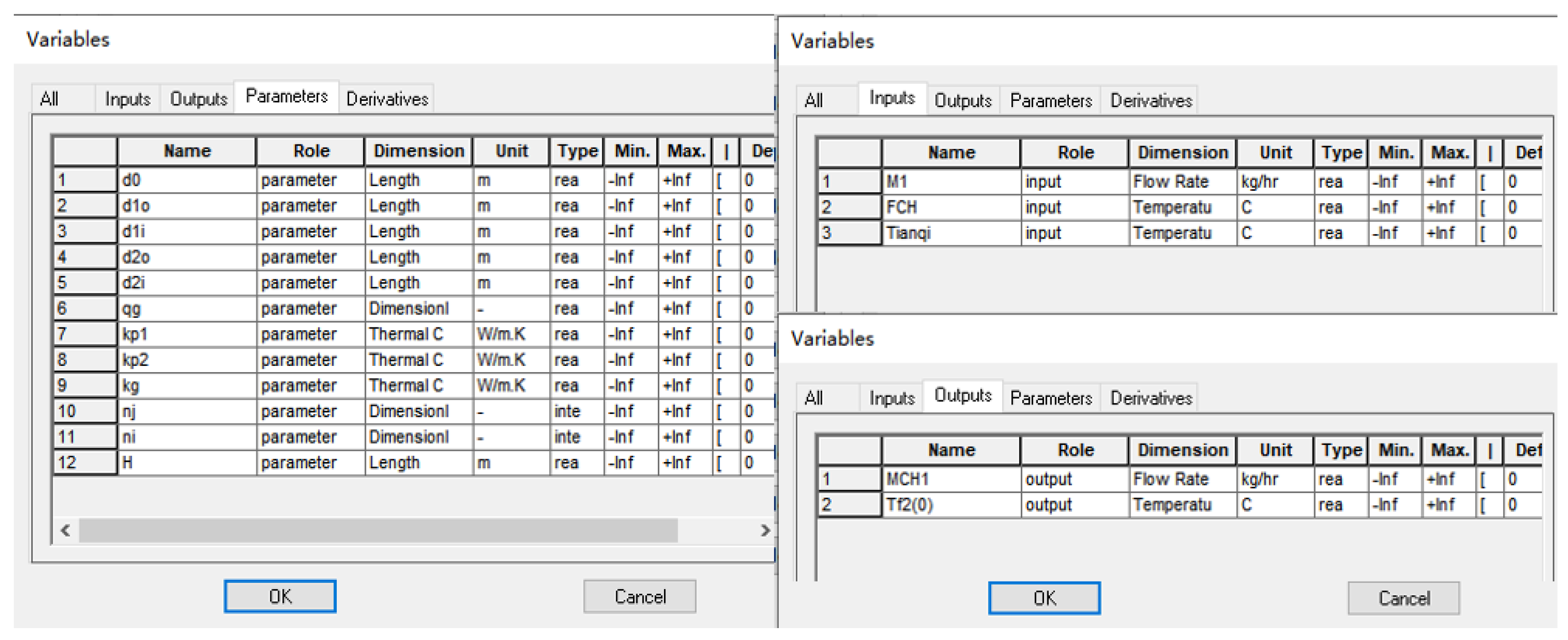
In order to allow the compiled program to successfully transfer data with other modules in TRNSYS, it is necessary to reasonably design the interface for data transfer between modules. The interface includes three tabs, as shown in
Figure 3.
There are three variables in the input tab: “FCH” represents the inlet water temperature; “M1” represents the flow rate of the circulating water; and “Tianqi” represents the local outdoor temperature.
There are two variables in the output tab: “MCH1” represents the flow rate of the circulating water, and “Tf2(0)” represents the outlet water temperature.
There are twelve variables in the Parameters tab: “d0” represents the diameter of the borehole; “d1o” represents the outer diameter of the outer pipe; “d1i” represents the inner diameter of the outer pipe; “d2o” represents the outer diameter of the inner pipe; “d2i” represents the inner diameter of the inner pipe; “qg” represents ground heat flow; “kp1” represents the thermal conductivity of the outer pipe; “kp2” represents the thermal conductivity of the inner pipe; “kg” represents the thermal conductivity of the geotechnical layers; “ni” represents the number of transverse nodes; “nj” represents the number of longitudinal nodes; and “H” represents the well depth of the buried-pipe heat exchanger.
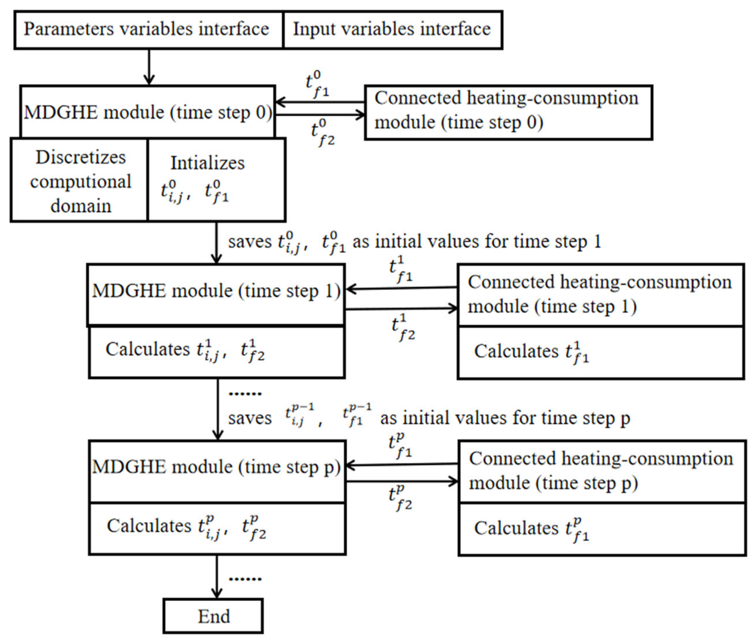
Upon configuring the parameters of the buried-pipe heat exchanger, we successfully established the Type282 module within the Type Studio environment of TRNSYS. A computational flowchart of the module within the TRNSYS environment is depicted in
Figure 4. The following steps were conducted:
At time step 0, the MDGHE module reads data from its parameter variables and input variables interfaces. A heating consumption module is connected to the MDGHE module. The outlet water temperature
is transferred from the MDGHE module to the heating consumption module, and the water temperature is returned to the MDGHE module after heating is consumed in the heating consumption module. is the temperature of a discrete point with the transverse serial number i and longitudinal serial number j. and are assigned to be 0 and saved as the initial values for time step 1. is assigned to be the original temperature of the geotechnical layers and saved as the initial value for time step 1.
At time step 1, the MDGHE module calculates and based on and . is transferred from the MDGHE module to the heating consumption module, and the water temperature is returned to the MDGHE module after heating is consumed in the heating-consumption module; this temperature is calculated based on and the heating load. , , and are saved as the initial values for time step 2.
Continuing the process, at time step p, the MDGHE module calculates and based on and . Then, is transferred from the MDGHE module to the heating-consumption module, and the water temperature is returned to the MDGHE module after heating is consumed in the heating consumption module; this temperature is calculated based on and the heating load. , , and are saved as the initial values for time step p+1.
2.5. Experimental Validation
In this study, the accuracy of the simulation results was validated using data obtained from a field experiment conducted in the Liuhong community, Dezhou City, Shandong Province.
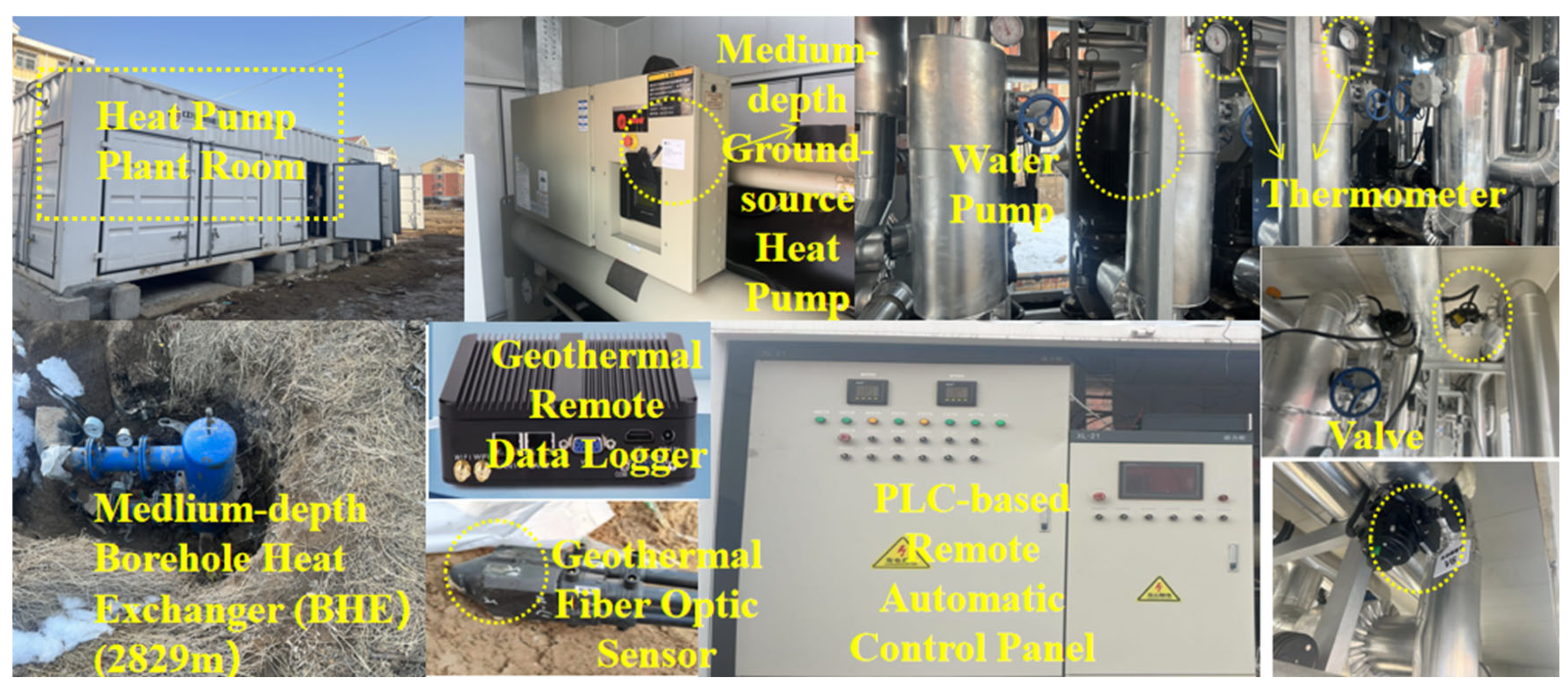
The experimental system was built based on the MDGHE ground source heat pump system in the studied case, to be rebuilt as a solar-assisted MDGHE system for direct heating. The in situ experimental system comprised the middle-depth ground heat exchanger (MDGHE), the automatic control system, and other equipment located in the plant room, as illustrated in
Figure 5. It should be noted that this experiment only uses the operation data of the MDGHE to verify the developed heat transfer model of MDGHE.
The MDGHE was retrofitted from a decommissioned geothermal well with a depth of 2829 m. As depicted in
Figure 6, the ground heat exchanger is composed of four sections. The structural parameters for these four sections are detailed in
Table 2.
The remaining parameters were configured as follows: The outer pipe was made of steel and had a thermal conductivity of 43 W/(m·K). The circulating medium within the buried pipe was water, flowing at a rate of 20 m3/h. The average ambient temperature was maintained at 15 °C. The backfill material has a thermal conductivity of 1.5 W/(m·K). For the inner pipe, PVC was selected, which has a thermal conductivity of 0.17 W/(m·K).
The in situ measurement of underground soil temperature was carried out using fiber optic sensors. These sensors are capable of four-channel fiber optic temperature sensing. Each channel has a detection distance of over 5 km and offers a temperature measurement accuracy of ±0.5 °C. The distributed temperature sensing (DTS) system was installed along the borehole, with temperature sensing points spaced every 0.5 m, enabling continuous monitoring down to a depth of 800 m. The ground temperature gradient was estimated to be 0.027 °C/m through data fitting, as illustrated in
Figure 7. Based on this gradient, the temperature at a depth of 2829 m was inferred to be 79.8 °C, extrapolated from the temperature measured at a depth of 800 m.
In this demonstration project, an automatic inspection system was designed and implemented within the PLC automatic control cabinet (as shown in
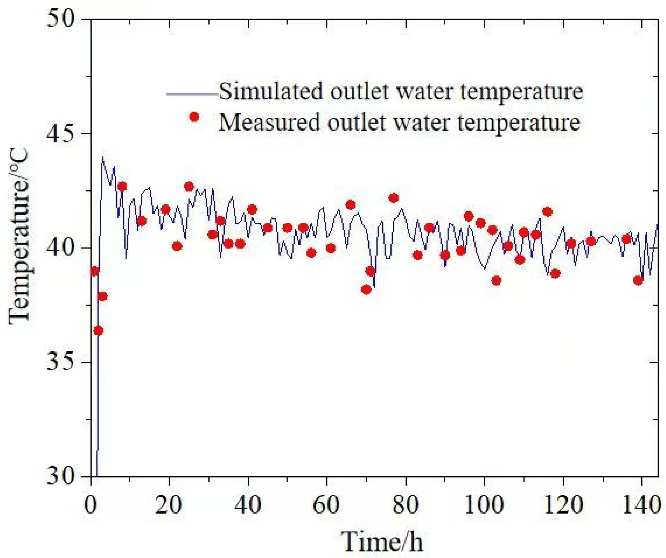
Figure 5). This system automatically recorded the inlet water temperature, outlet water temperature, and circulating water flow rate of the MDGHE. Based on these recorded data, the capacity of the heat exchanger under heating conditions was calculated. Additionally, on the load side, the supply temperature, return temperature, circulating water flow rate, and circulating pump power were also automatically recorded. The same parameters used in the experimental system were input into the TRNSYS module for simulation and analysis. A load-based outlet temperature validation method was employed in this study. The validation process involved the following steps: (1) The instantaneous thermal load was calculated from the measured inlet and outlet water temperatures and the flow rate. (2) This calculated heat load was used as input for the numerical module to estimate the corresponding outlet water temperature. (3) The calculated outlet temperature was then compared with the experimentally measured value to assess the model’s accuracy.
Figure 8 presents a comparison between the simulated and measured outlet water temperatures. The results indicate that the error range is within ±2.5 °C except for the initial 5 h, which is caused by initial static water temperature. This demonstrates the acceptable accuracy of the developed TRNSYS module for MDGHE simulations. The potential errors of this experiment may come from the following aspects: (1) The measurement accuracy of the optical fiber sensor has affected the accuracy. (2) Due to the relatively short experimental period, some thermal inertial response processes were not fully reflected in the data. (3) Although the pipeline has been insulated, due to the large fluctuations in outdoor temperature, heat loss still exists, and there will be errors in the calculation process.
2.6. The Model’s Limitations and a Sensitivity Analysis
2.6.1. The Model’s Limitations
This study focused on heat transfer in a single deep borehole with coaxial tubes. The following assumptions were taken into account in the model:
The soil and rock surrounding the DBHE is regarded as one or a few horizontal layers of homogeneous media, whose thermal properties do not change with temperature.
The domain studied is considered semi-infinite; for numerical simulation, however, boundaries are set far away from the DBHE, where temperature distributions are assumed to be uninfluenced by DBHE operation in the period concerned.
Groundwater infiltration is neglected, and pure conduction is considered the only mechanism of heat transfer in the soil/rock.
The fluctuation in the temperature of the atmosphere and its influence on the top layer of the soil are ignored, so the air temperature above the ground surface remains constant.
A uniform geothermal heat flux exists throughout the media.
Convective heat transport by circulating water in pipes is the dominant mechanism of heat transfer in the longitudinal direction within the borehole; conduction by grout, pipe walls, and water in the borehole is neglected in this direction.
The thermal capacity of the grout, pipe walls, and water in pipes is counted in the model; the temperature of the grout and pipe walls, however, is assumed to be the same as that of the water in the same section of the pipe.
2.6.2. Sensitivity Analysis
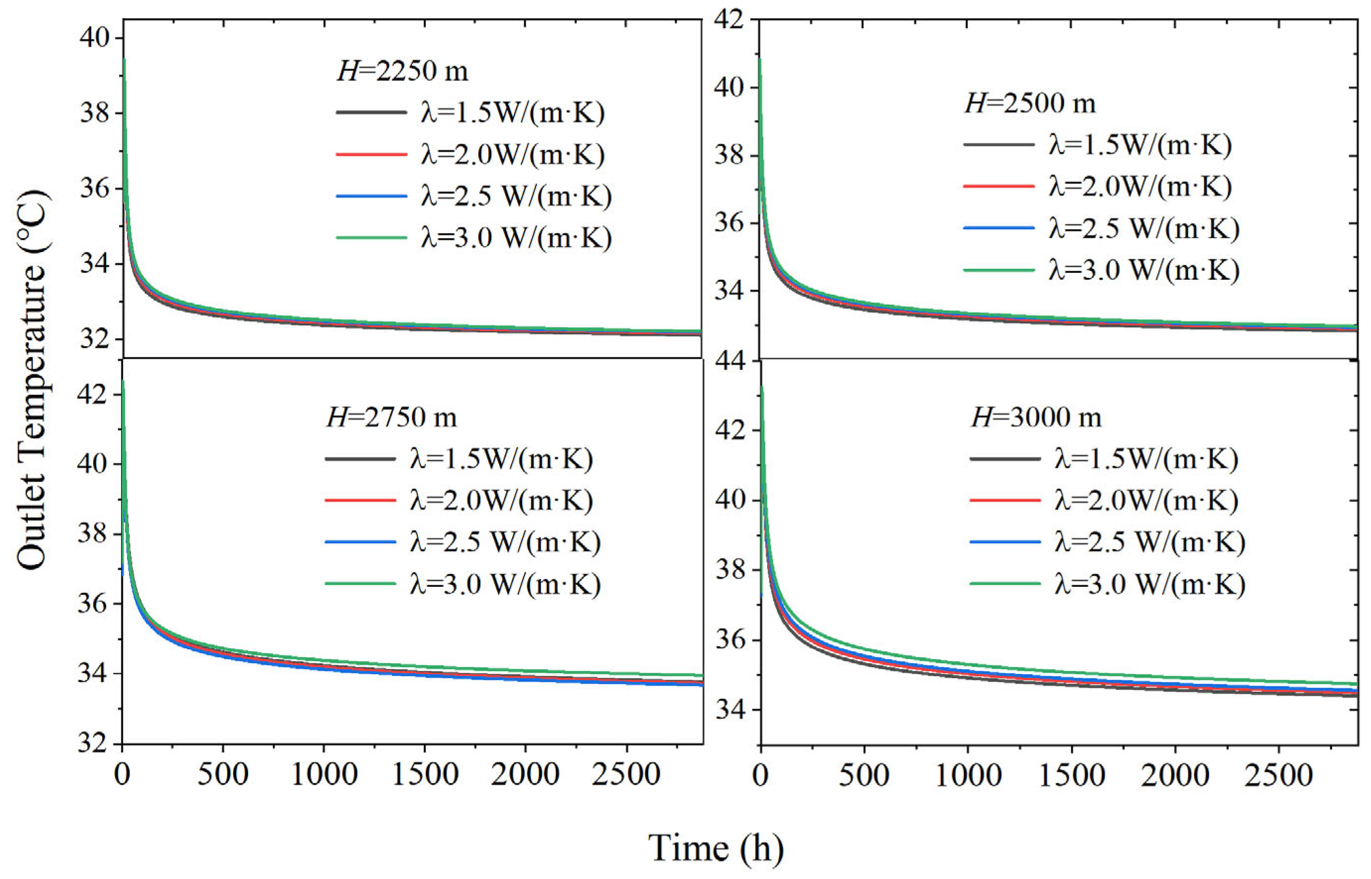
The effects of two key parameters, borehole depth and soil thermal conductivity, on the variation in the outlet water temperature of an MDGHE were investigated, clarifying the importance of the role of each parameter in the thermal response of the system. The parameters of the MDGHE were set to be the same as those in
Table 2. The inlet water temperature was taken to be 30 °C, and the flow rate was 60 m
3/h.
The trend of the system outlet water temperature over the operating time can be clearly observed by comparing the simulation results at different depths (2250–3000 m) and under different soil thermal conductivity (1.5–3.0 W/(m·K)) conditions, see
Figure 9. The results of the analysis show that the outlet water temperature exhibited a trend of rapidly increasing in the early stage of system operation, but with the increase in the heat extraction time, the outlet water temperature of the buried-pipe heat exchanger gradually decreased and eventually stabilized. This phenomenon indicates that the heat exchange between the soil and the fluid stabilizes, and the system can reach thermal dynamic equilibrium when it operates for longer periods of time. It can also be seen from the figure that the effect of borehole depth on outlet water temperature is particularly significant, with a maximum temperature rise 3.6 °C. This phenomenon is due to the fact that as depth increases, the temperature of the geothermal field gradually rises, thus enhancing the heat exchange capacity between the fluid in the pipe and the surrounding soil.
In contrast, the effect of soil thermal conductivity on the thermal performance of the system was relatively weak. Increasing the thermal conductivity from 1.5 W/(m·K) to 3.0 W/(m·K) at the same depth resulted in an increase of 0.2 °C in outlet water temperature. Although the increase in thermal conductivity can accelerate the rate at which thermal energy is conducted through the soil to the fluid, the effect on the outlet water temperature is significantly weakened by the fact that the ground temperature gradient is mainly determined by the natural conditions of the ground and the fact that the heat transfer time is relatively long. Overall, the outlet water temperature is highly sensitive to the depth of the borehole, and the response to the change in soil thermal conductivity is weak. Therefore, in the design and optimization of medium-depth buried-pipe heat transfer systems, the depth of the borehole should be considered a key parameter that must be prioritized, and geothermal heat collection efficiency should be improved by reasonably increasing the depth of the borehole to achieve a higher energy utilization rate.
3. Development of a TRNSYS Simulation Framework for a Solar-Assisted MDGHE Direct Heating System
Following the development of the MDGHE model, we aimed to evaluate the performance of the solar-assisted MDGHE direct heating system by integrating the newly developed module into the TRNSYS simulation framework.
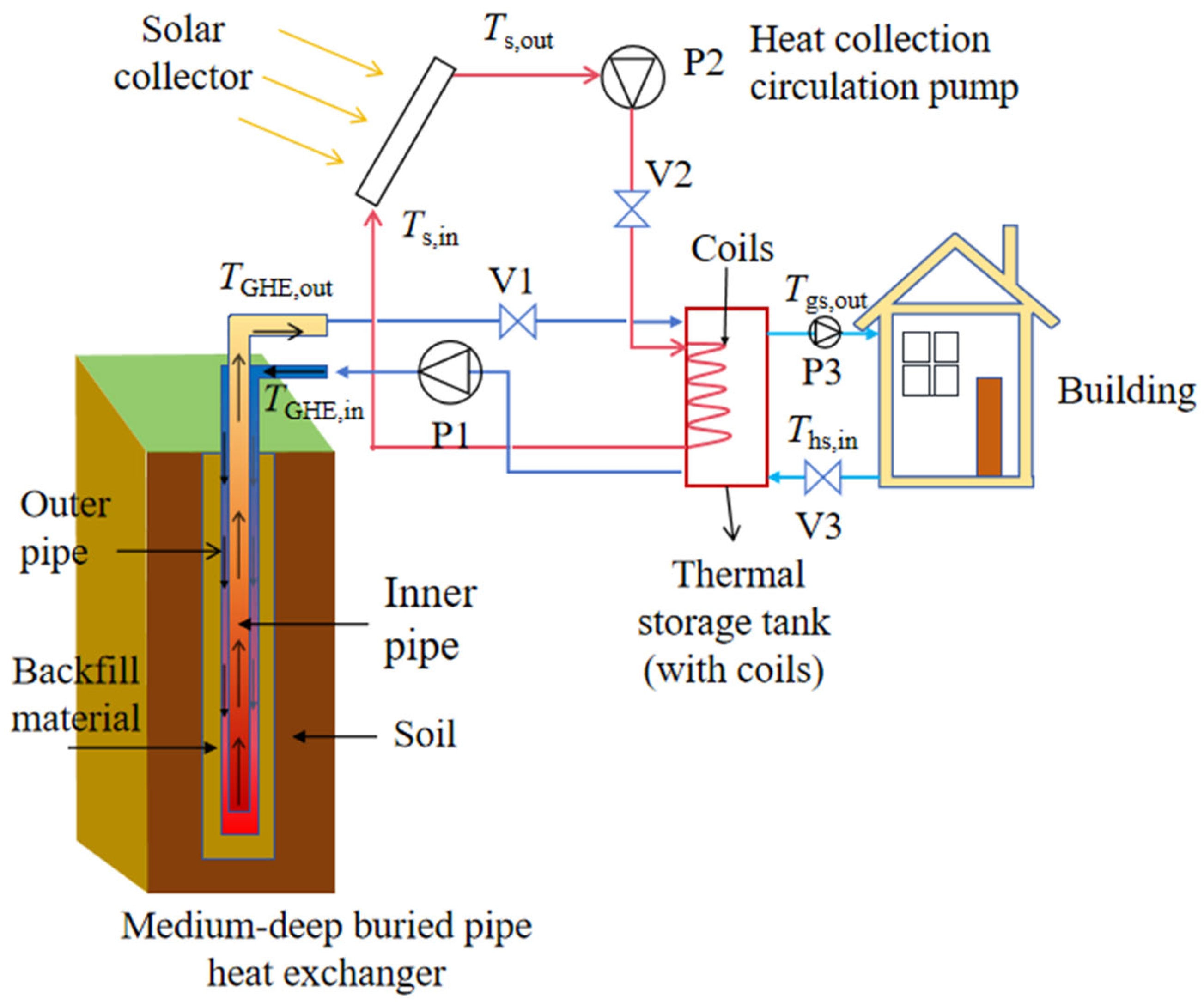
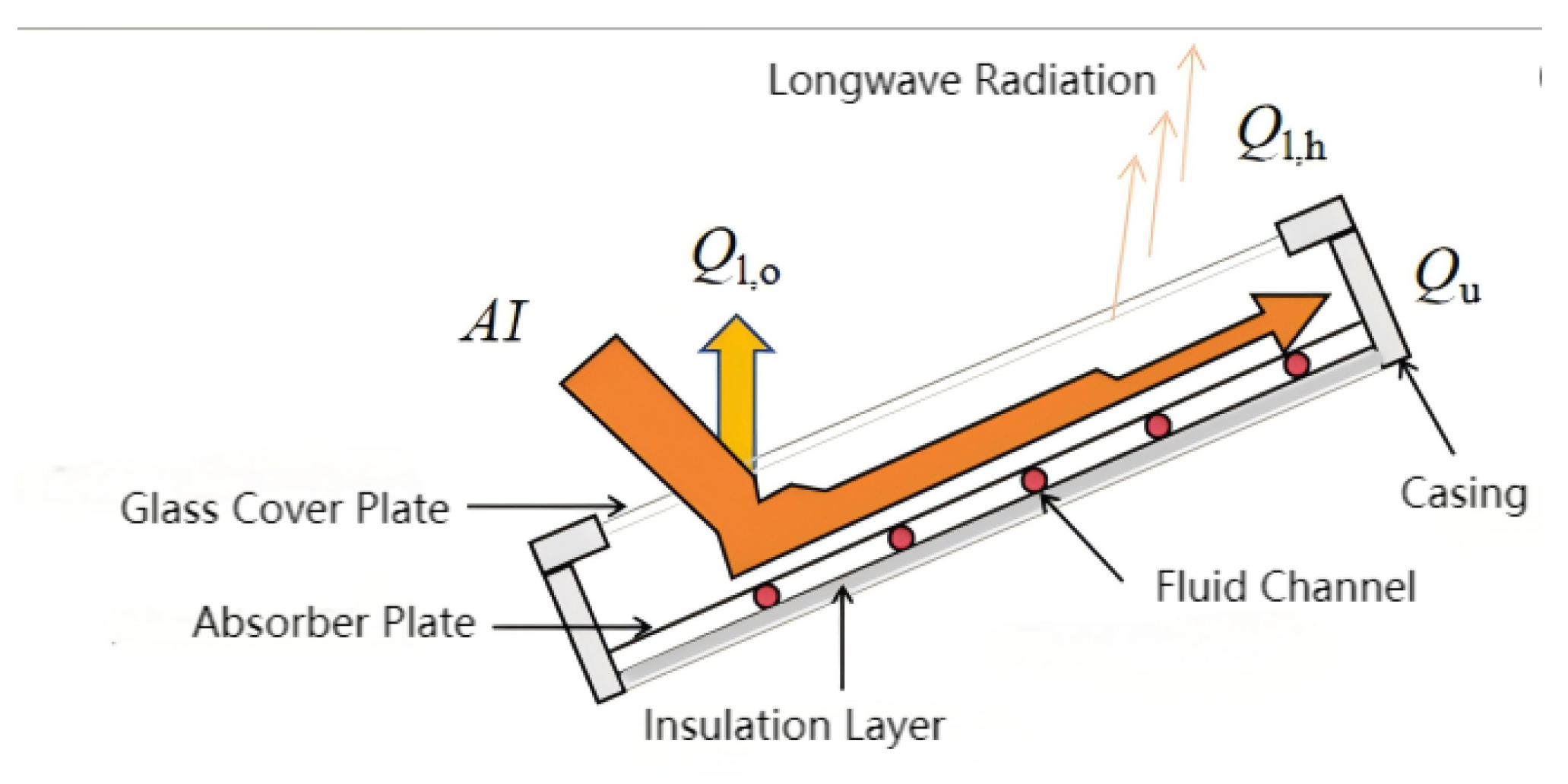
Figure 10 is a schematic diagram of the solar-assisted MDGHE direct heating system. The integrated heating system incorporates four core subsystems: (1) an MDGHE, (2) flat-plate solar collectors, (3) a stratified thermal storage unit with an internal heat exchanger, and (4) low-temperature radiant heating terminals.
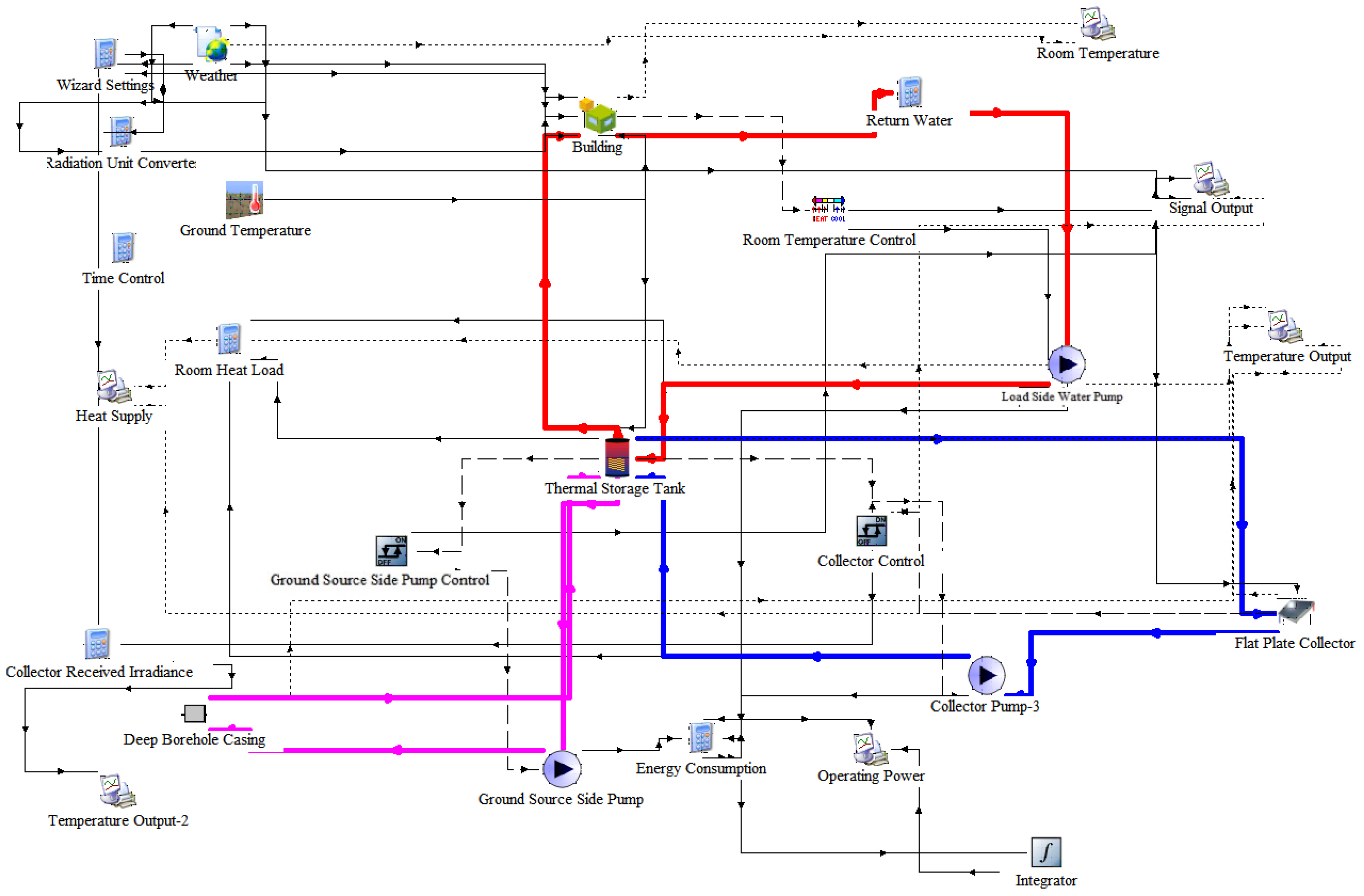
Following the system design specifications, the corresponding components were systematically selected and interconnected within the TRNSYS simulation environment in order to develop a comprehensive numerical model. As illustrated in
Figure 11, the implemented model consists of the following parts:
- (1)
Component selection: accurate matching of numerical modules with physical components, along with customized parameterization for each subsystem.
- (2)
System integration: thermodynamic coupling of all energy transfer processes, hydraulic connection establishment, and control logic implementation.
- (3)
Model configuration: time-step optimization, convergence criteria setting, and output parameter definition.
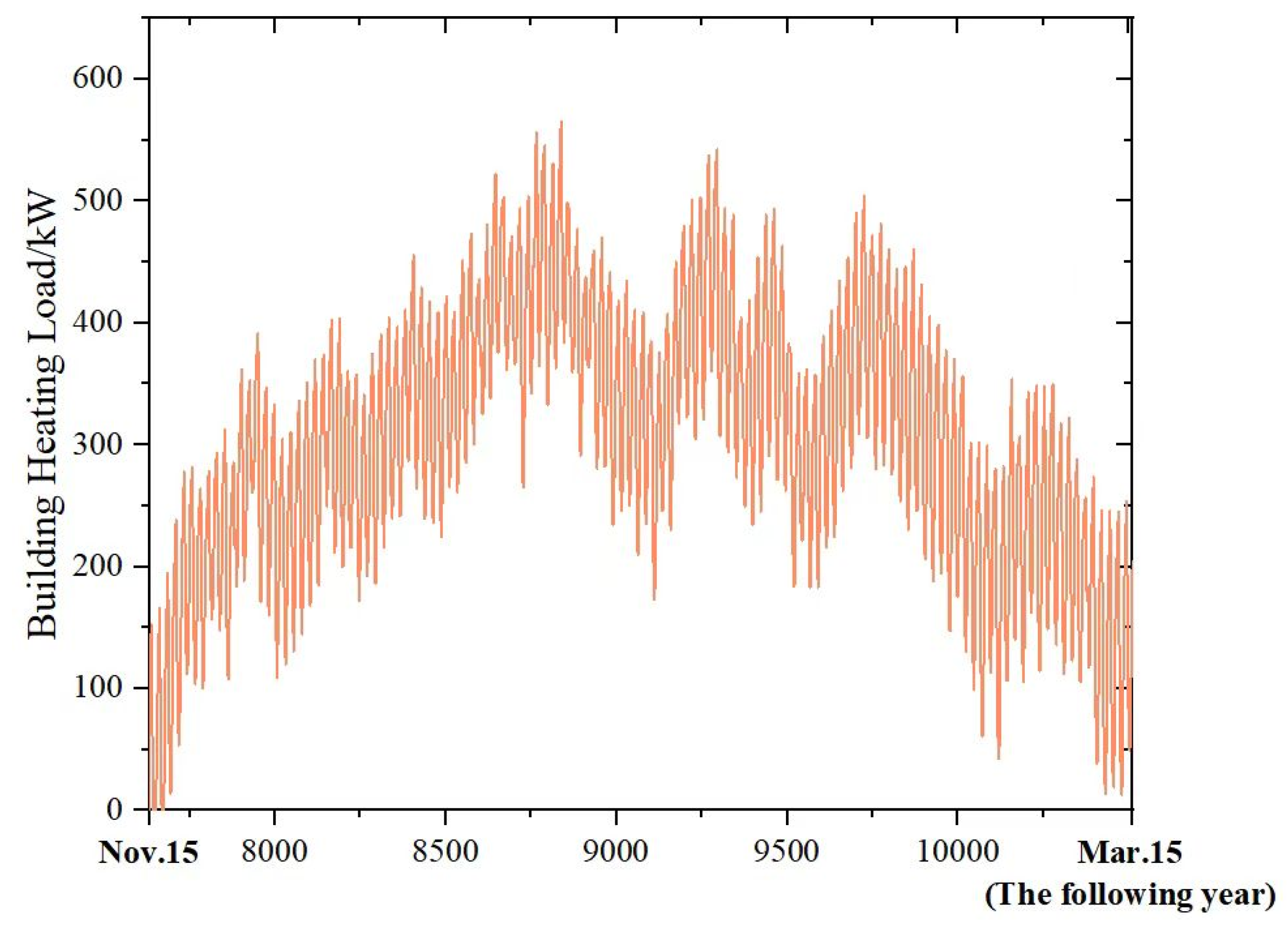
3.1. Building Heating Load Simulation
The heating load profile of a residential building with an area of 12,000 m2 was simulated using the Type 56 module in TRNSYS. The accuracy of simulation results largely depends on the appropriateness of a model’s boundary conditions and parameter settings. The conditions and parameter settings used for the simulation are presented below.
- (1)
Outdoor meteorological parameters
Load simulations were conducted using Typical Meteorological Year (TMY) data. The TMY was determined by statistically analyzing the monthly averages of meteorological data over the past 30 years, selecting the most representative year from the most recent decade that best approximated the 30-year monthly averages. The geolocation settings for the software were set to Dezhou, Shandong Province, to extract local meteorological data.
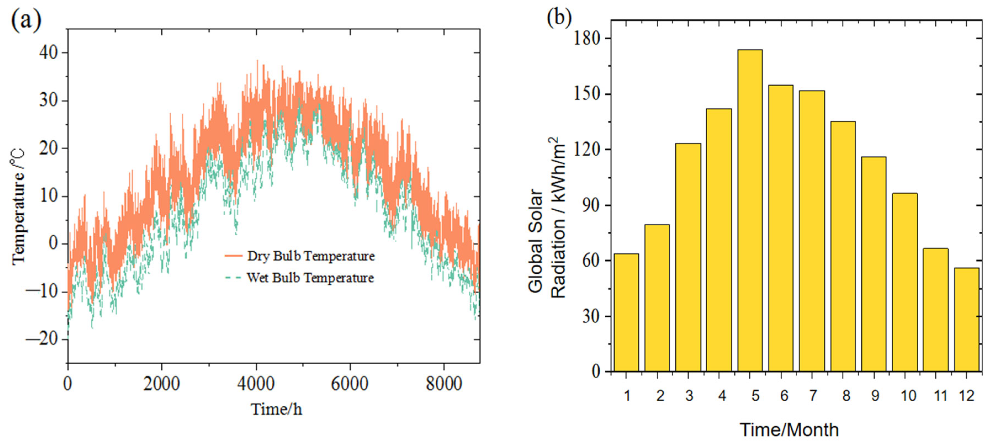
Dezhou (37°45′ N, 116°3′ E), located in the central region of Shandong Province, has a warm temperate semi-humid continental monsoon climate, characterized by hot, rainy summers and cold, dry winters. The multi-year average temperature is 14.3 °C. The seasonal variations in outdoor temperature and solar radiation intensity are illustrated in
Figure 12.
- (2)
Building Envelope Parameters
The configuration of the envelope and the window-to-wall ratios (WWRs) for each orientation are detailed in the following sections.
Table 3 presents the thermal parameters of the residential building envelope, while
Table 4 specifies the WWR values across various facades.
- (3)
Additional parameter configurations
The indoor thermal conditions were controlled, with indoor temperature and relative humidity setpoints of 20 °C and 50%, respectively. Standard fluorescent lamps were selected for lighting, with radiant and convective heat fluxes set at 5.4 kW·h/m2 and 3.6 kW·h/m2, respectively. Electrical appliances were set to a power density of 280 W, while the ventilation system operated at an air exchange rate of 0.5/h. Continuous 24 h heating operation was implemented, with a simulated occupant load of three people for heating load calculations.
3.2. Determination of Equipment Capacity
The developed numerical algorithms for the MDGHE were computationally implemented as a customized TRNSYS simulation module. The detailed parameters of the MDGHE module, which can solve 70% of the peak heating load, are shown in
Table 5.
A type 1b component was used to simulate a flat-plate solar collector. The thermal performance of the flat-plate collector array depends on the number of connected collectors and the thermal performance of each individual collector. The collector component allows users to customize parameters such as the total collector area, installation angle, collection efficiency, and circulating fluid flow rate.
The collector outlet fluid temperature can be calculated by incorporating the known basic parameters of the collector together with the local hourly solar radiation intensity and the inlet fluid temperature (as shown in
Figure 13).
The gradually increasing solar collector area was integrated with the MDGHE, and the area measuring 1231 m
2 was selected when indoor temperature reached over 99.9% of the heating time. The parameters of the flat-plate solar collector are shown in
Table 6.
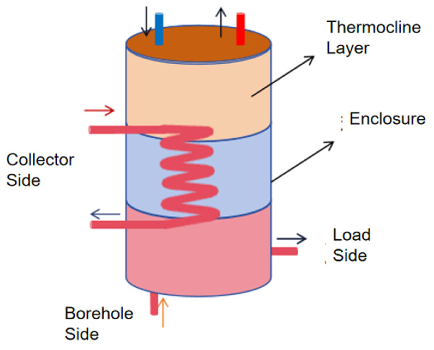
In this study, antifreeze was used as a circulating fluid to prevent freezing in the solar collectors. Pure water was used as the heat exchange medium in the storage tank. To prevent the mixing of the antifreeze and water, a storage tank with an internal coil heat exchanger was used in the system. The heat storage tank with a coil heat exchanger is shown in
Figure 14.
The volume of a storage tank is typically selected based on the unit area of the collector. Typically, the range is between 40 L/m
2 and 300 L/m
2, as recommended by the Chinese “Technical standard for solar heating system (GB50495-2019)” [
32]. In this study, we assumed that the volume of the storage tank is equal to 100 L per square meter of collector area. The detailed parameters of the thermal storage tank are shown in
Table 7.
The parameters of circulating pumps on solar side, MDGHE side and load side are shown in
Table 8.
3.3. Control Strategies
The performance of a solar-assisted MDGHE system can be significantly influenced by the applied control strategies. In this study, optimized operational control strategies for essential components were developed to ensure heating stability and comfort while maximizing energy efficiency. The details of these strategies are presented below.
- (1)
Control strategies for the circulating pumps on the solar side: We employed a temperature-difference-based control strategy in which pump operation is regulated by monitoring the temperature difference between the temperature of the solar collector and the temperature of the return water of the water tank. Specifically, when the temperature of the solar collector exceeds the water tank return water temperature by 8 °C, the circulating pump is activated to transfer the collected solar heat to the water tank. Conversely, when the temperature difference drops below the set threshold of 2 °C, the circulating pump is deactivated to prevent heat backflow, which would otherwise reduce the system’s energy efficiency.
- (2)
Control strategies for the circulating pumps on the MDGHE side: The system establishes a minimum water supply temperature of 35 °C to meet the requirements for direct heating. When the solar heating contribution is inadequate, resulting in the heat storage tank temperature falling below 35 °C, the system will activate the pipe circulation pump on the MDGHE side to introduce geothermal energy into the heating process.
- (3)
Control strategies for circulating pumps on the load side: The indoor temperature is carefully controlled and maintained between 19 and 21 °C. When the temperature drops below 19 °C, the circulating pumps on the load side are activated to heat the room. Conversely, when the temperature rises above 21 °C, the circulating pumps on the load side are deactivated to prevent overheating.


 and
and 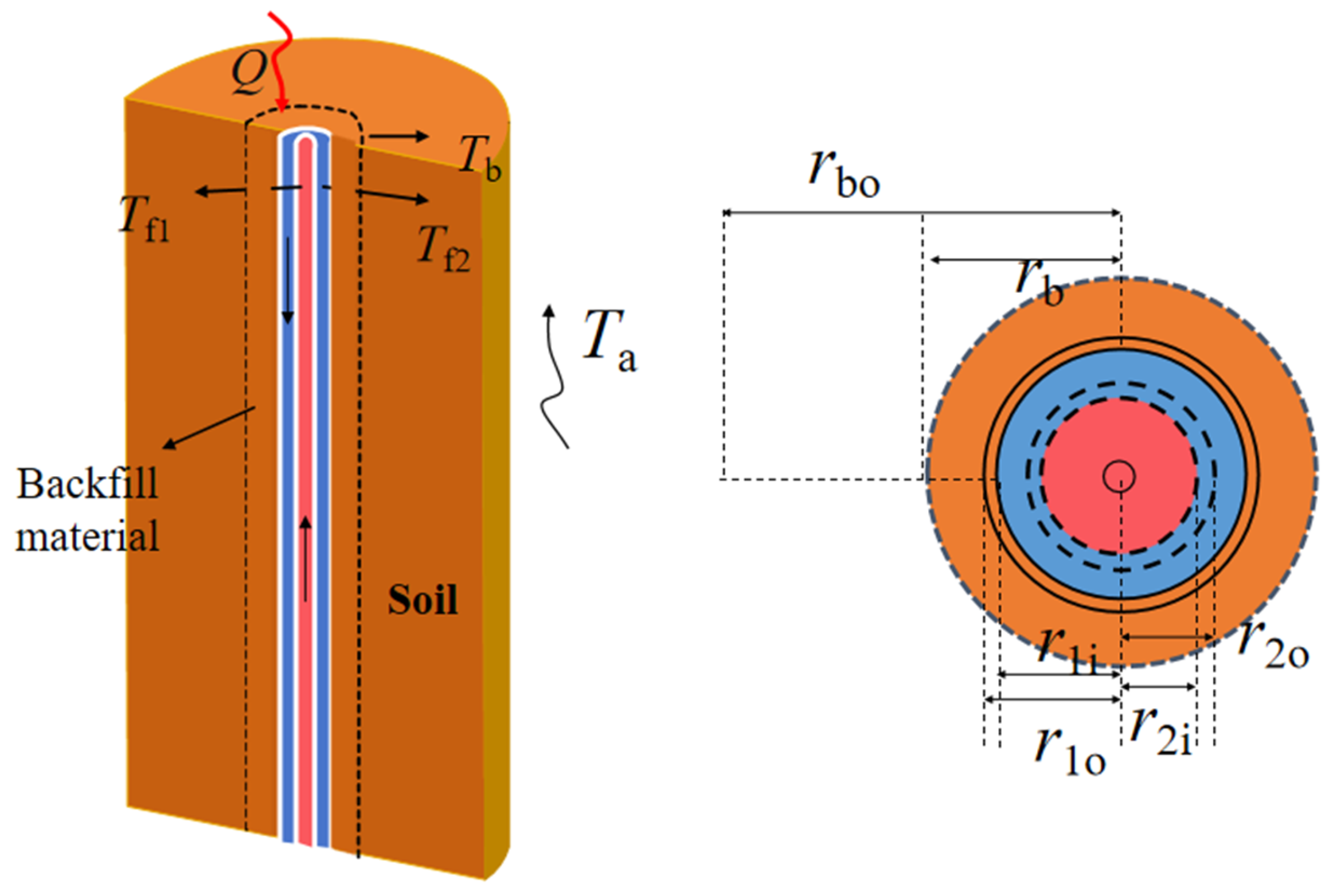


