
Which Distance-Decay Function Can Improve the Goodness of Fit of the Metro Station Ridership Regression Model? A Case Study of Beijing


Abstract
1. Introduction
2. Literature Review
2.1. PCA Determination of Metro Stations
2.2. Distance-Decay Function in Built Environment Calculation
2.3. Explanatory Variables for the Built Environment
2.4. Methods for Analyzing the Impact of the Built Environment on Ridership
2.5. Current Gaps and Our Study
3. Methods
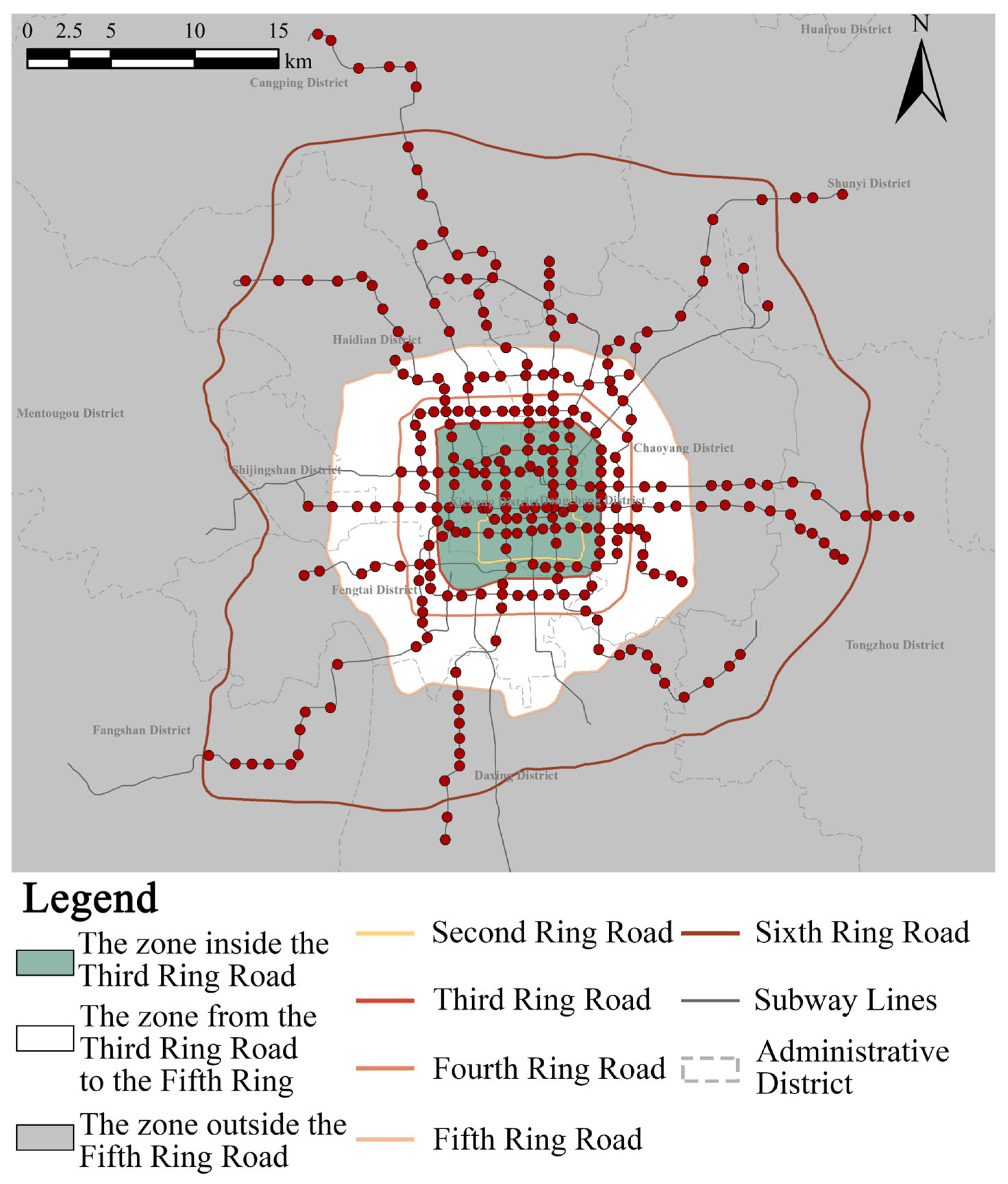
3.1. Study Scope
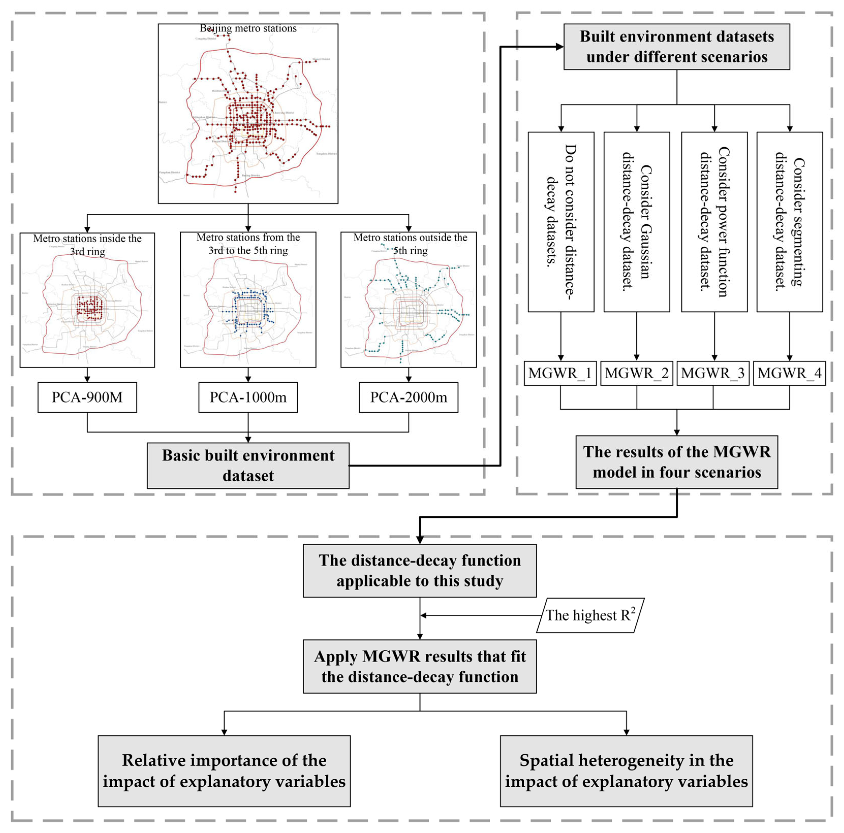
3.2. Research Framework
3.3. The Delineation of the PCA at the Metro Station
3.4. Construction and Preprocessing of Built Environment Explanatory Variables
3.4.1. Built Environment Explanatory Variables and Data Source
3.4.2. Distance-Decay Function
3.4.3. Data Processing and Variable Calculation
3.5. Analysis Methods for the Impact of the Built Environment on Ridership
3.5.1. Multicollinearity Test
3.5.2. Multi-Scale Geographically Weighted Regression (MGWR)
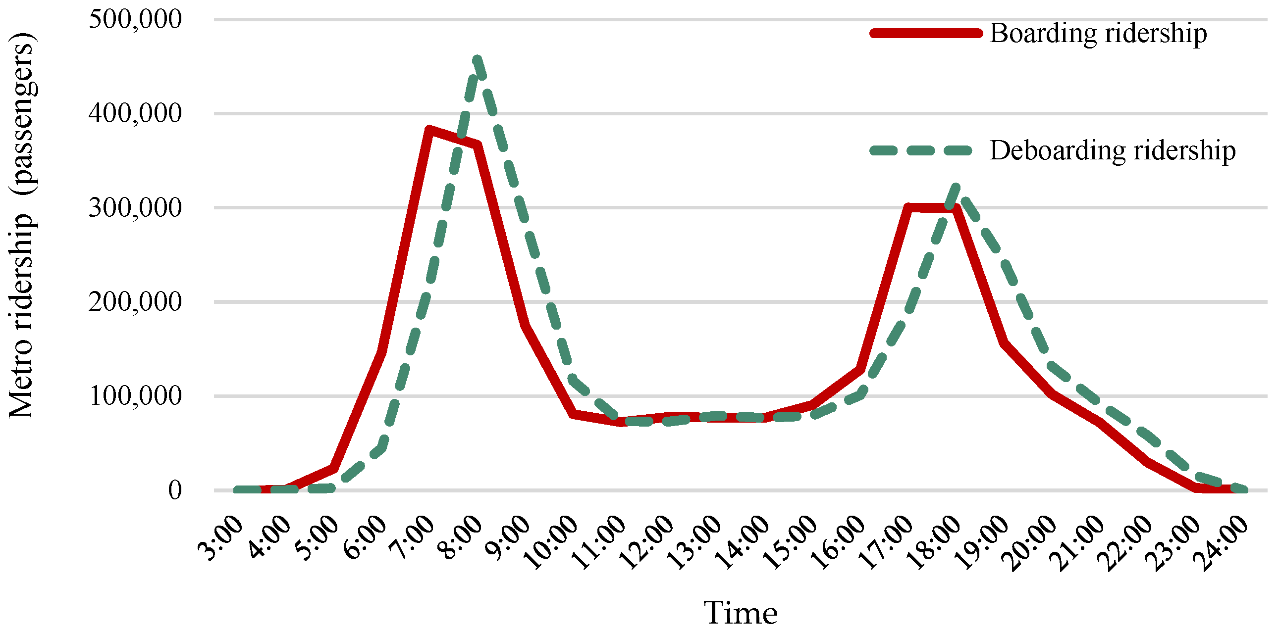
4. Results
4.1. Effect of Different Distance-Decay Functions on Model Accuracy
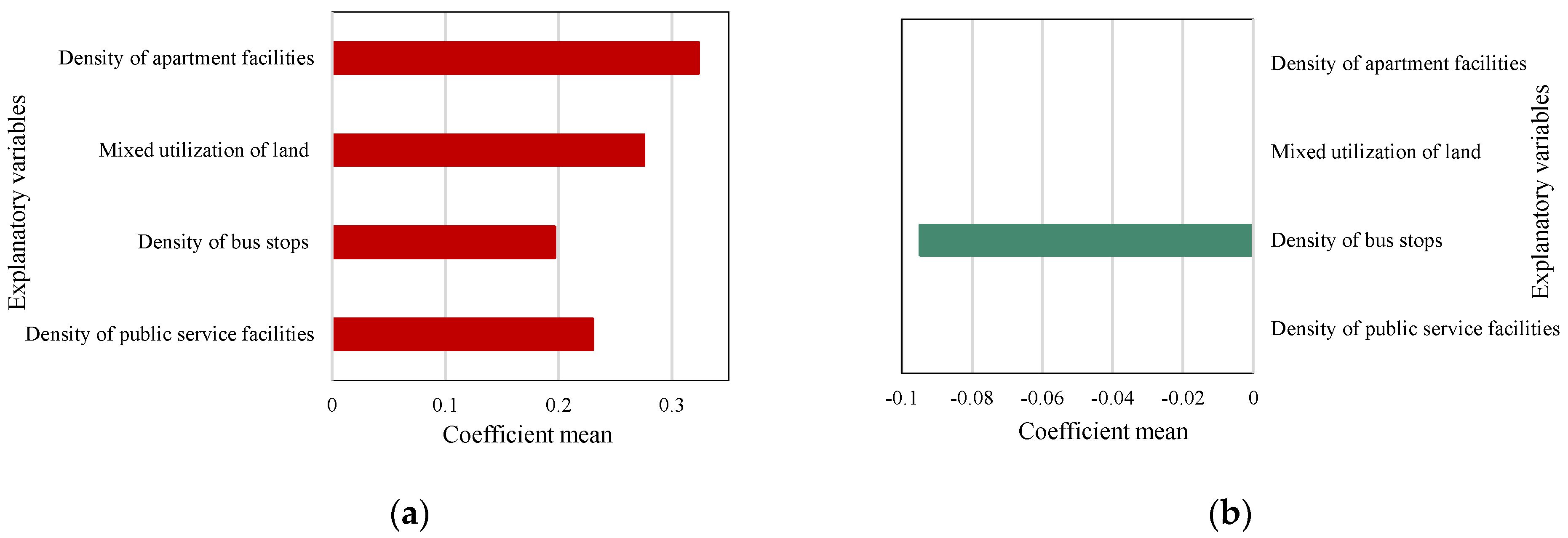
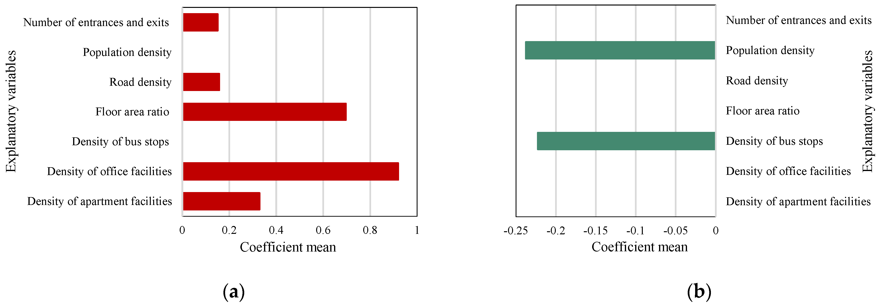
4.2. The Overall Impact of Built Environment Explanatory Variables
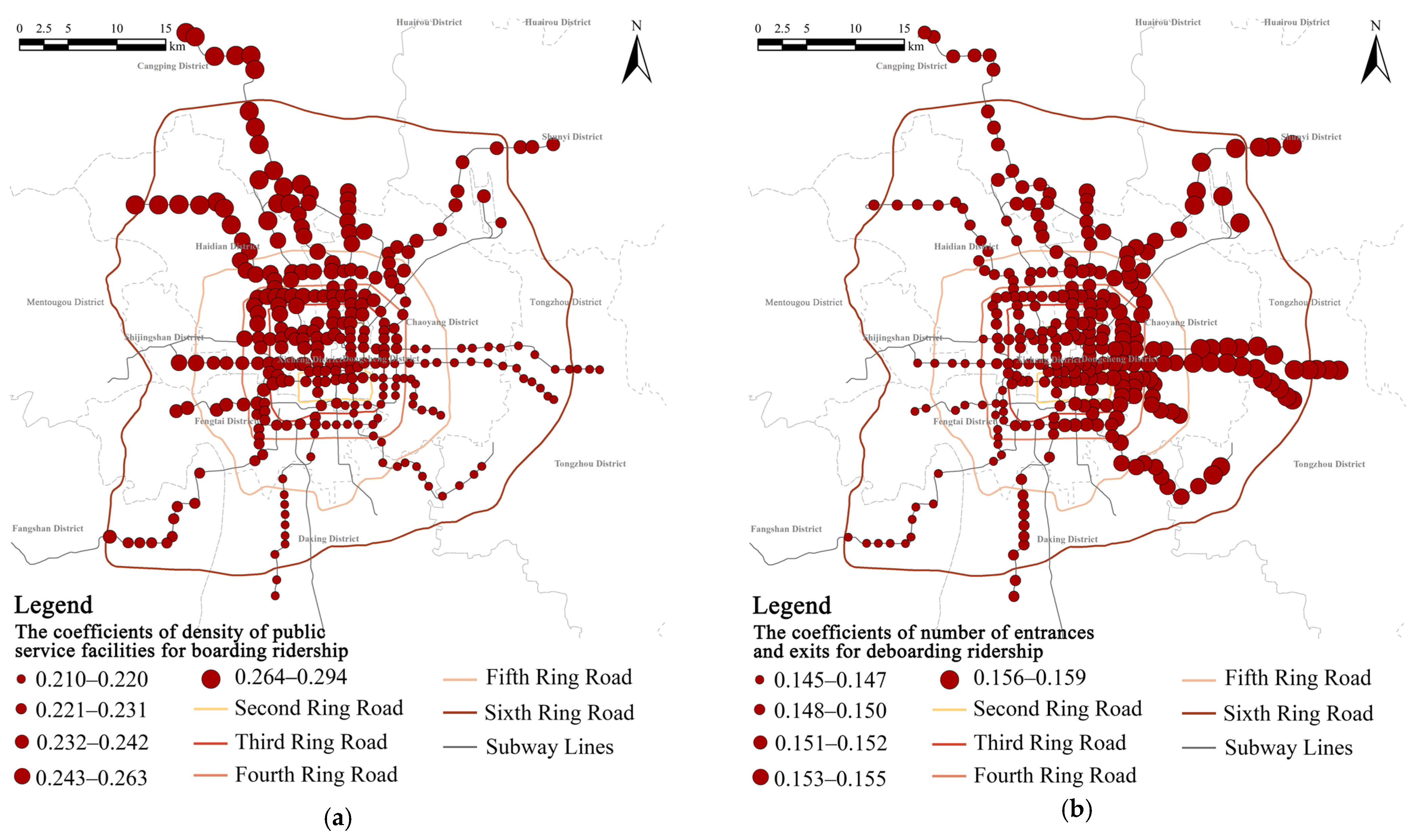
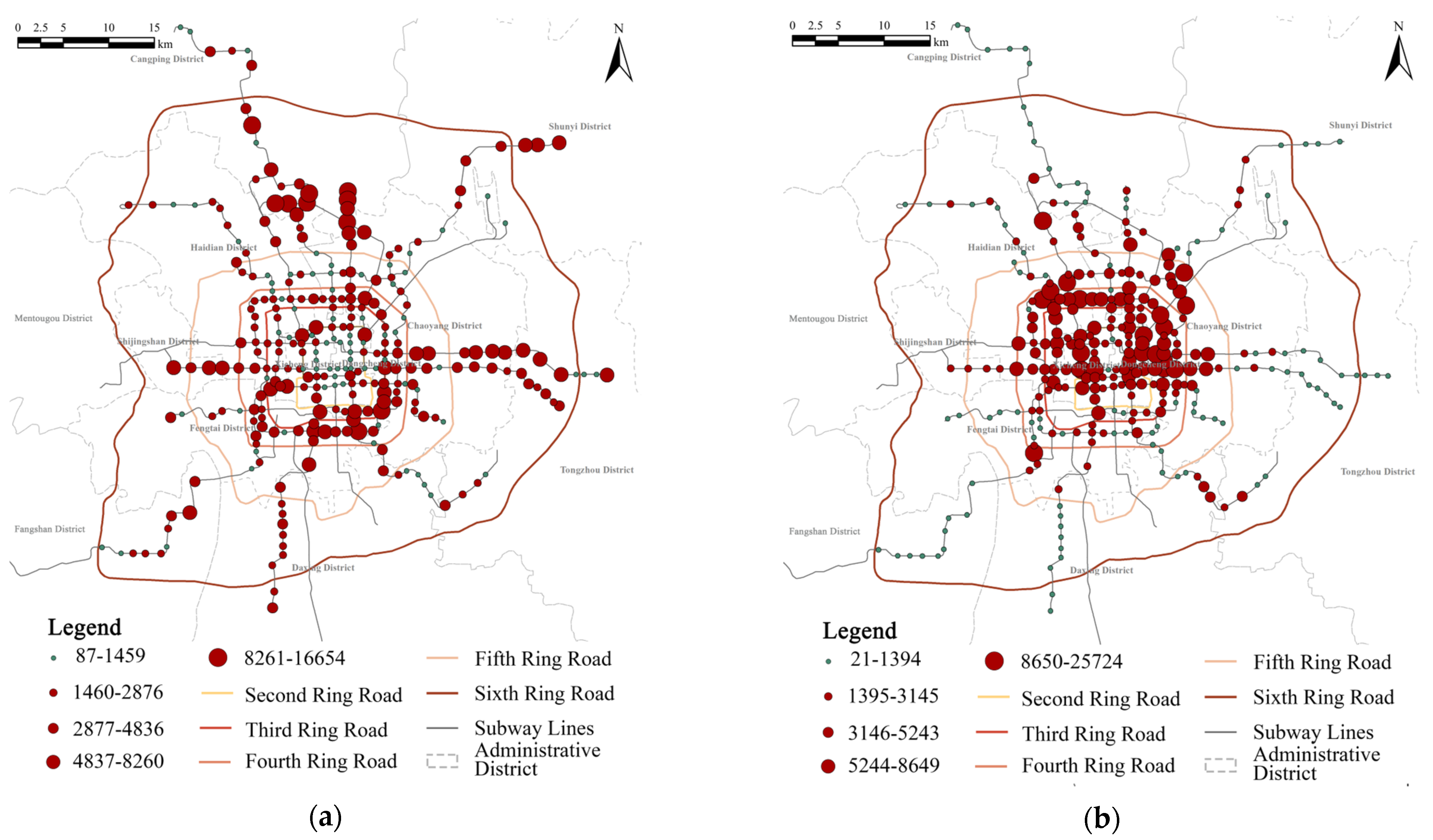
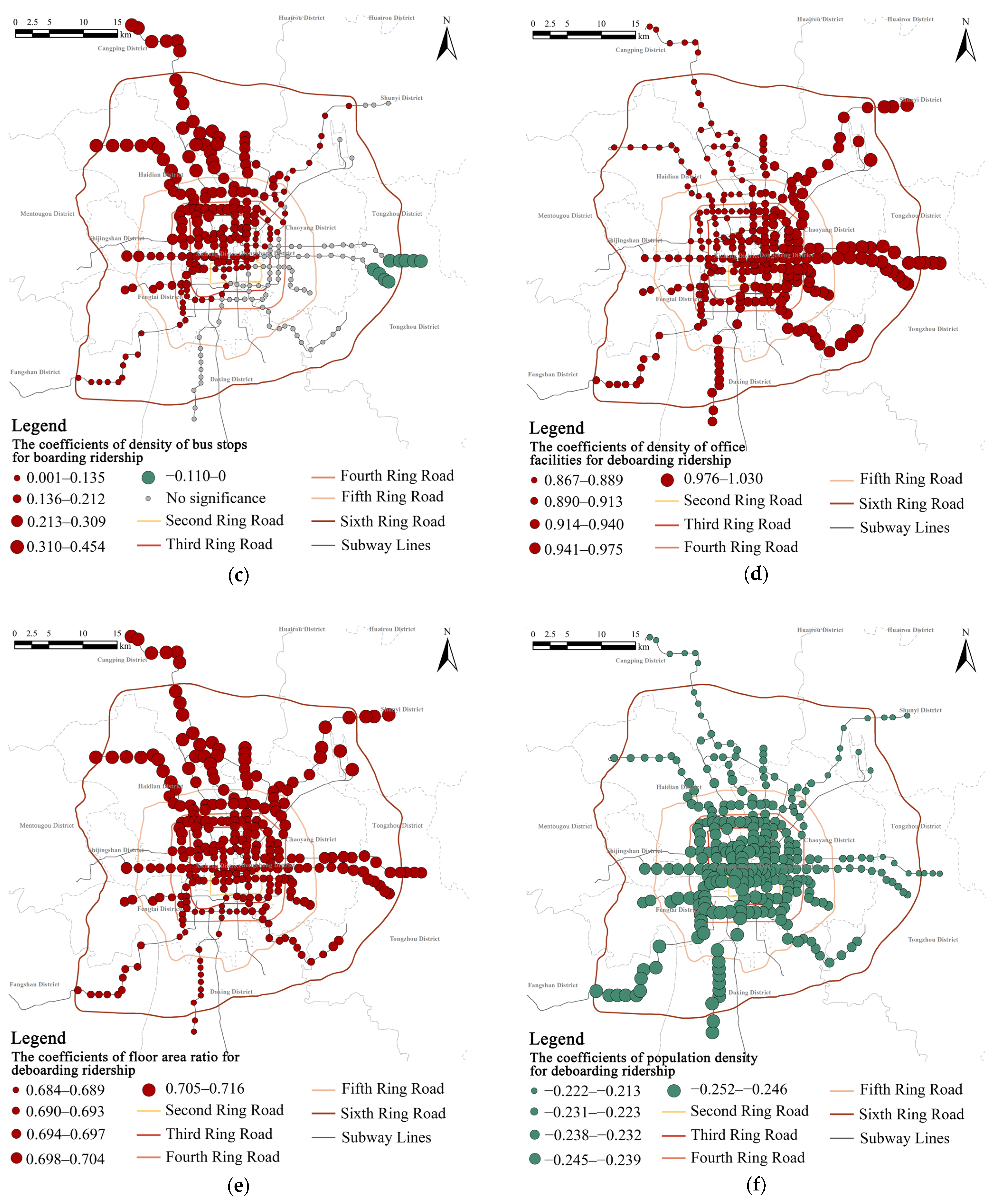
4.3. Spatial Heterogeneity of the Impact of the Built Environment on Metro Ridership
5. Discussion
5.1. Evaluating Distance-Decay Functions in Metro Ridership Modeling
5.2. The Influence of Built Environment on Metro Ridership Under Distance-Decay
5.3. Policy Implications
6. Conclusions
Author Contributions
Funding
Data Availability Statement
Conflicts of Interest
Appendix A

References
- Sung, H.; Choi, K.; Lee, S.; Cheon, S. Exploring the impacts of land use by service coverage and station-level accessibility on rail transit ridership. J. Transp. Geogr. 2014, 36, 134–140. [Google Scholar] [CrossRef]
- Chiou, Y.-C.; Jou, R.-C.; Yang, C.-H. Factors affecting public transportation usage rate: Geographically weighted regression. Transp. Res. Part A Policy Pract. 2015, 78, 161–177. [Google Scholar] [CrossRef]
- Zhao, J.; Deng, W.; Song, Y.; Zhu, Y. What influences Metro station ridership in China? Insights from Nanjing. Cities 2013, 35, 114–124. [Google Scholar] [CrossRef]
- Li, S.; Liu, X.; Li, Z.; Wu, Z.; Yan, Z.; Chen, Y.; Gao, F. Spatial and Temporal Dynamics of Urban Expansion along the Guangzhou–Foshan Inter-City Rail Transit Corridor, China. Sustainability 2018, 10, 593. [Google Scholar] [CrossRef]
- Shen, Q.; Chen, P.; Pan, H. Factors affecting car ownership and mode choice in rail transit-supported suburbs of a large Chinese city. Transp. Res. Part A Policy Pract. 2016, 94, 31–44. [Google Scholar] [CrossRef]
- Cervero, R.; Day, J. Suburbanization and transit-oriented development in China. Transp. Policy 2008, 15, 315–323. [Google Scholar] [CrossRef]
- Beijing Youth Daily. Passenger Flow Gradually Picked Up, and Some Subway Stations in Beijing Temporarily Restricted Traffic Outside the Morning Rush Hour Station. Available online: https://m.163.com/dy/article/HTMVP1I20514R9KQ.html (accessed on 12 April 2025).
- Zhao, J.; Deng, W.; Song, Y.; Zhu, Y. Analysis of Metro ridership at station level and station-to-station level in Nanjing: An approach based on direct demand models. Transportation 2013, 41, 133–155. [Google Scholar] [CrossRef]
- Gan, Z.; Yang, M.; Feng, T.; Timmermans, H.J.P. Examining the relationship between built environment and metro ridership at station-to-station level. Transp. Res. Part D Transp. Environ. 2020, 82, 102332. [Google Scholar] [CrossRef]
- Li, S.; Lyu, D.; Huang, G.; Zhang, X.; Gao, F.; Chen, Y.; Liu, X. Spatially varying impacts of built environment factors on rail transit ridership at station level: A case study in Guangzhou, China. J. Transp. Geogr. 2020, 82, 102631. [Google Scholar] [CrossRef]
- Wang, Z.; Li, S.; Li, Y.; Liu, D.; Liu, S.; Chen, N. Investigating the Nonlinear Effect of Built Environment Factors on Metro Station-Level Ridership under Optimal Pedestrian Catchment Areas via the Machine Learning Method. Appl. Sci. 2023, 13, 12210. [Google Scholar] [CrossRef]
- Jun, M.-J.; Choi, K.; Jeong, J.-E.; Kwon, K.-H.; Kim, H.-J. Land use characteristics of subway catchment areas and their influence on subway ridership in Seoul. J. Transp. Geogr. 2015, 48, 30–40. [Google Scholar] [CrossRef]
- Zhang, S.; Li, Z.; Liu, Z.; Guo, R.-Y. Examining Built Environment Effects on Metro Ridership at Station-to-Station Level considering Circle Heterogeneity: A Case Study from Xi’an, China. J. Adv. Transp. 2023, 2023, 4597386. [Google Scholar] [CrossRef]
- Li, S.; Lyu, D.; Liu, X.; Tan, Z.; Gao, F.; Huang, G.; Wu, Z. The varying patterns of rail transit ridership and their relationships with fine-scale built environment factors: Big data analytics from Guangzhou. Cities 2020, 99, 102580. [Google Scholar] [CrossRef]
- Liu, M.; Liu, Y.; Ye, Y. Nonlinear effects of built environment features on metro ridership: An integrated exploration with machine learning considering spatial heterogeneity. Sustain. Cities Soc. 2023, 95, 104613. [Google Scholar] [CrossRef]
- Du, Q.; Zhou, Y.; Huang, Y.; Wang, Y.; Bai, L. Spatiotemporal exploration of the non-linear impacts of accessibility on metro ridership. J. Transp. Geogr. 2022, 102, 103380. [Google Scholar] [CrossRef]
- Shao, Q.; Zhang, W.; Cao, X.; Yang, J.; Yin, J. Threshold and moderating effects of land use on metro ridership in Shenzhen: Implications for TOD planning. J. Transp. Geogr. 2020, 89, 102878. [Google Scholar] [CrossRef]
- Kuby, M.; Barranda, A.; Upchurch, C. Factors influencing light-rail station boardings in the United States. Transp. Res. Part A Policy Pract. 2004, 38, 223–247. [Google Scholar] [CrossRef]
- Jiang, Y.; Christopher Zegras, P.; Mehndiratta, S. Walk the line: Station context, corridor type and bus rapid transit walk access in Jinan, China. J. Transp. Geogr. 2012, 20, 1–14. [Google Scholar] [CrossRef]
- Sohn, K.; Shim, H. Factors generating boardings at Metro stations in the Seoul metropolitan area. Cities 2010, 27, 358–368. [Google Scholar] [CrossRef]
- Sung, H.; Oh, J.-T. Transit-oriented development in a high-density city: Identifying its association with transit ridership in Seoul, Korea. Cities 2011, 28, 70–82. [Google Scholar] [CrossRef]
- Cardozo, O.D.; García-Palomares, J.C.; Gutiérrez, J. Application of geographically weighted regression to the direct forecasting of transit ridership at station-level. Appl. Geogr. 2012, 34, 548–558. [Google Scholar] [CrossRef]
- Estupiñán, N.; Rodríguez, D.A. The relationship between urban form and station boardings for Bogotá’s BRT. Transp. Res. Part A Policy Pract. 2008, 42, 296–306. [Google Scholar] [CrossRef]
- Liu, J.; Wang, B.; Xiao, L. Non-linear associations between built environment and active travel for working and shopping: An extreme gradient boosting approach. J. Transp. Geogr. 2021, 92, 103034. [Google Scholar] [CrossRef]
- Ding, C.; Cao, X.; Liu, C. How does the station-area built environment influence Metrorail ridership? Using gradient boosting decision trees to identify non-linear thresholds. J. Transp. Geogr. 2019, 77, 70–78. [Google Scholar] [CrossRef]
- Andersson, D.E.; Shyr, O.F.; Yang, J. Neighbourhood effects on station-level transit use: Evidence from the Taipei metro. J. Transp. Geogr. 2021, 94, 103127. [Google Scholar] [CrossRef]
- Zhao, J.; Deng, W. Relationship of Walk Access Distance to Rapid Rail Transit Stations with Personal Characteristics and Station Context. J. Urban Plan. Dev. 2013, 139, 311–321. [Google Scholar] [CrossRef]
- Guerra, E.; Cervero, R.; Tischler, D. Half-Mile Circle. Transp. Res. Rec. J. Transp. Res. Board 2012, 2276, 101–109. [Google Scholar] [CrossRef]
- He, J.; Zhang, R.; Huang, X.; Xi, G. Walking Access Distance of Metro Passengers and Relationship with Demographic Characteristics: A Case Study of Nanjing Metro. Chin. Geogr. Sci. 2018, 28, 612–623. [Google Scholar] [CrossRef]
- Jia, P.; Wang, F.; Xierali, I.M. Differential effects of distance decay on hospital inpatient visits among subpopulations in Florida, USA. Environ. Monit. Assess. 2019, 191, 381. [Google Scholar] [CrossRef]
- Kang, J.Y.; Michels, A.; Lyu, F.; Wang, S.; Agbodo, N.; Freeman, V.L.; Wang, S. Rapidly measuring spatial accessibility of COVID-19 healthcare resources: A case study of Illinois, USA. Int. J. Health Geogr. 2020, 19, 36. [Google Scholar] [CrossRef]
- Wang, F. Measurement, Optimization, and Impact of Health Care Accessibility: A Methodological Review. Ann. Assoc. Am. Geogr. 2012, 102, 1104–1112. [Google Scholar] [CrossRef] [PubMed]
- Chen, B.Y.; Cheng, X.-P.; Kwan, M.-P.; Schwanen, T. Evaluating spatial accessibility to healthcare services under travel time uncertainty: A reliability-based floating catchment area approach. J. Transp. Geogr. 2020, 87, 102794. [Google Scholar] [CrossRef]
- Gutiérrez, J.; Cardozo, O.D.; García-Palomares, J.C. Transit ridership forecasting at station level: An approach based on distance-decay weighted regression. J. Transp. Geogr. 2011, 19, 1081–1092. [Google Scholar] [CrossRef]
- Gao, K.; Yang, Y.; Li, A.; Qu, X. Spatial heterogeneity in distance decay of using bike sharing: An empirical large-scale analysis in Shanghai. Transp. Res. Part D Transp. Environ. 2021, 94, 102814. [Google Scholar] [CrossRef]
- Hipp, J.R.; Boessen, A. The Shape of Mobility: Measuring the Distance Decay Function of Household Mobility. Prof. Geogr. 2016, 69, 32–44. [Google Scholar] [CrossRef]
- De Vries, J.J.; Nijkamp, P.; Rietveld, P. Exponential or Power Distance-Decay for Commuting? An Alternative Specification. Environ. Plan. A Econ. Space 2009, 41, 461–480. [Google Scholar] [CrossRef]
- Dong, Q.; Zeng, P.; Long, X.; Peng, M.; Tian, T.; Che, Y. An improved accessibility index to effectively assess urban park allocation: Based on working and residential situations. Cities 2024, 145, 104736. [Google Scholar] [CrossRef]
- Li, A.; Huang, Y.; Axhausen, K.W. An approach to imputing destination activities for inclusion in measures of bicycle accessibility. J. Transp. Geogr. 2020, 82, 102566. [Google Scholar] [CrossRef]
- Thompson, G.; Brown, J.; Bhattacharya, T. What Really Matters for Increasing Transit Ridership: Understanding the Determinants of Transit Ridership Demand in Broward County, Florida. Urban Stud. 2012, 49, 3327–3345. [Google Scholar] [CrossRef]
- Calvo, F.; Eboli, L.; Forciniti, C.; Mazzulla, G. Factors influencing trip generation on metro system in Madrid (Spain). Transp. Res. Part D Transp. Environ. 2019, 67, 156–172. [Google Scholar] [CrossRef]
- Li, D.; Zang, H.; Yu, D.; He, Q.; Huang, X. Study on the Influence Mechanism and Space Distribution Characteristics of Rail Transit Station Area Accessibility Based on MGWR. Int. J. Environ. Res. Public Health 2023, 20, 1535. [Google Scholar] [CrossRef] [PubMed]
- Zhu, P.; Li, J.; Wang, K.; Huang, J. Exploring spatial heterogeneity in the impact of built environment on taxi ridership using multiscale geographically weighted regression. Transportation 2023, 51, 1963–1997. [Google Scholar] [CrossRef]
- Li, X.; Yan, Q.; Ma, Y.; Luo, C. Spatially Varying Impacts of Built Environment on Transfer Ridership of Metro and Bus Systems. Sustainability 2023, 15, 7891. [Google Scholar] [CrossRef]
- Gu, Y.; Dou, M. Nonlinear and Threshold Effects on Station-Level Ridership: Insights from Disproportionate Weekday-to-Weekend Impacts. ISPRS Int. J. Geo-Inf. 2024, 13, 365. [Google Scholar] [CrossRef]
- Loo, B.P.Y.; Chen, C.; Chan, E.T.H. Rail-based transit-oriented development: Lessons from New York City and Hong Kong. Landsc. Urban Plan. 2010, 97, 202–212. [Google Scholar] [CrossRef]
- Cervero, R.; Kockelman, K. Travel demand and the 3Ds: Density, diversity, and design. Transp. Res. Part D Transp. Environ. 1997, 2, 199–219. [Google Scholar] [CrossRef]
- Ewing, R.; Cervero, R. Travel and the built environment—A synthesis. Transp. Res. Rec. 2001, 1870, 87–114. [Google Scholar] [CrossRef]
- Ewing, R.; Cervero, R. Travel and the Built Environment. J. Am. Plan. Assoc. 2010, 76, 265–294. [Google Scholar] [CrossRef]
- Xi, Y.; Hou, Q.; Duan, Y.; Lei, K.; Wu, Y.; Cheng, Q. Exploring the Spatiotemporal Effects of the Built Environment on the Nonlinear Impacts of Metro Ridership: Evidence from Xi’an, China. ISPRS Int. J. Geo-Inf. 2024, 13, 105. [Google Scholar] [CrossRef]
- Yang, H.; Zhang, Q.; Wen, J.; Sun, X.; Yang, L. Multi-group exploration of the built environment and metro ridership: Comparison of commuters, seniors and students. Transp. Policy 2024, 155, 189–207. [Google Scholar] [CrossRef]
- Huang, Y.; Zhang, Z.; Xu, Q.; Dai, S.; Chen, Y. Causality between multi-scale built environment and rail transit ridership in Beijing and Tokyo. Transp. Res. Part D Transp. Environ. 2024, 130, 104150. [Google Scholar] [CrossRef]
- Wang, Z.; Li, S.; Zhang, Y.; Wang, X.; Liu, S.; Liu, D. Built Environment Renewal Strategies Aimed at Improving Metro Station Vitality via the Interpretable Machine Learning Method: A Case Study of Beijing. Sustainability 2024, 16, 1178. [Google Scholar] [CrossRef]
- Lu, B.; Yang, W.; Ge, Y.; Harris, P. Improvements to the calibration of a geographically weighted regression with parameter-specific distance metrics and bandwidths. Comput. Environ. Urban Syst. 2018, 71, 41–57. [Google Scholar] [CrossRef]
- Chen, E.; Ye, Z.; Wang, C.; Zhang, W. Discovering the spatio-temporal impacts of built environment on metro ridership using smart card data. Cities 2019, 95, 102359. [Google Scholar] [CrossRef]
- Wang, W.; Wang, H.; Liu, J.; Liu, C.; Wang, S.; Zhang, Y. Estimating Rail Transit Passenger Flow Considering Built Environment Factors: A Case Study in Shenzhen. Appl. Sci. 2024, 14, 799. [Google Scholar] [CrossRef]
- Fotheringham, A.S.; Yang, W.; Kang, W. Multiscale Geographically Weighted Regression (MGWR). Ann. Am. Assoc. Geogr. 2017, 107, 1247–1265. [Google Scholar] [CrossRef]
- Li, P.; Yang, Q.; Lu, W.; Xi, S.; Wang, H. An Improved Machine Learning Framework Considering Spatiotemporal Heterogeneity for Analyzing the Relationship Between Subway Station-Level Passenger Flow Resilience and Land Use-Related Built Environment. Land 2024, 13, 1887. [Google Scholar] [CrossRef]
- Ding, Z.; Chen, E.; Teng, J. Discovering impacts of built environment on transit ridership in the post-COVID era: Policy intervention and nonlinear dynamics. Int. J. Transp. Sci. Technol. 2025, in press. [Google Scholar] [CrossRef]
- Zhang, S.; Zhang, J.; Yang, Y.; Kong, Y.; Li, Z.; Shen, Y.; Tang, J. The non-linear effects of built environment on bus ridership of vulnerable people. Transp. Res. Part D Transp. Environ. 2025, 139, 104540. [Google Scholar] [CrossRef]
- Dai, D. Black residential segregation, disparities in spatial access to health care facilities, and late-stage breast cancer diagnosis in metropolitan Detroit. Health Place 2010, 16, 1038–1052. [Google Scholar] [CrossRef]
- Tao, Z.L.; Cheng, Y.; Dai, T.Q.; Rosenberg, M.W. Spatial optimization of residential care facility locations in Beijing, China: Maximum equity in accessibility. Int. J. Health Geogr. 2014, 13, 33. [Google Scholar] [CrossRef] [PubMed]
- Kim, Y.; Byon, Y.J.; Yeo, H. Enhancing healthcare accessibility measurements using GIS: A case study in Seoul, Korea. PLoS ONE 2018, 13, e0193013. [Google Scholar] [CrossRef] [PubMed]
- Mansour, S.; Al Kindi, A.; Al-Said, A.; Al-Said, A.; Atkinson, P. Sociodemographic determinants of COVID-19 incidence rates in Oman: Geospatial modelling using multiscale geographically weighted regression (MGWR). Sustain. Cities Soc. 2021, 65, 102627. [Google Scholar] [CrossRef] [PubMed]
- Zhao, X.; Wu, Y.-p.; Ren, G.; Ji, K.; Qian, W.-w. Clustering Analysis of Ridership Patterns at Subway Stations: A Case in Nanjing, China. J. Urban Plan. Dev. 2019, 145, 04019005. [Google Scholar] [CrossRef]
- Lai, Y.; Zhou, J.; Xu, X. Spatial Relationships between Population, Employment Density, and Urban Metro Stations: A Case Study of Tianjin City, China. J. Urban Plan. Dev. 2024, 150, 05023048. [Google Scholar] [CrossRef]
- Han, H.; Yang, C.; Wang, E.; Song, J.; Zhang, M. Evolution of jobs-housing spatial relationship in Beijing Metropolitan Area: A job accessibility perspective. Chin. Geogr. Sci. 2015, 25, 375–388. [Google Scholar] [CrossRef]
- Huang, Y.; Du, Q.; Li, Y.; Li, J.; Huang, N. Effects of Metro Transit on the Job–Housing Balance in Xi’an, China. J. Urban Plan. Dev. 2022, 148, 04021068. [Google Scholar] [CrossRef]


| Explanatory Variables for the Built Environment | Dimension | Used by | Case Study |
|---|---|---|---|
| 3D | Density, Diversity, and Design | Cervero et al., 1997 [47] | San Francisco Bay Area, USA |
| 5D | Density, Diversity, Design, Destination accessibility, and Distance to transit | Ewing et al., 2001 [48] | California, USA |
| Xi et al., 2024 [50] | Xian, China | ||
| Yang et al., 2024 [51] | Kunming, China | ||
| Huang et al., 2024 [52] | Beijing, China and Tokyo, Japan | ||
| 7D | Density, Diversity, Design, Destination accessibility, Distance to transit, Demand management, and Demographics | Ewing et al., 2010 [49] | |
| Wang et al., 2023 [53] | Beijing, China |
| Built Environment Category | Interfering Factor | Descriptive Statistics (Without Considering the Decay Function) | Data Source | Unit | ||
|---|---|---|---|---|---|---|
| Max | Med | Min | ||||
| Density | Density of commercial facilities | 639.41 | 118.25 | 0.81 | https://lbs.amap.com, accessed on 10 October 2021 | quantity/km2 |
| Density of apartment facilities | 133.54 | 22.66 | 0.65 | |||
| Density of public service facilities | 102.59 | 18.38 | 0.16 | |||
| Density of office facilities | 990.85 | 112.64 | 3.09 | |||
| Floor area ratio | 3.72 | 1.23 | 0 | https://map.baidu.com, accessed on 10 October 2021 | ||
| Building density | 0.38 | 0.20 | 0 | https://map.baidu.com, accessed on 10 October 2021 | m2/km2 | |
| Diversity | Mixed utilization of land use | 1.25 | 1.09 | 0.42 | https://lbs.amap.com, accessed on 10 October 2021 | |
| Design | Road density | 14.36 | 6.10 | 0.26 | https://map.baidu.com, accessed on 10 October 2021 | km/km2 |
| Destination accessibility | Number of entrances and exits | 11 | 4 | 1 | https://www.bjsubway.com, accessed on 13 October 2020 | quantity |
| Distance to transit | Density of bus lines | 127.69 | 33.14 | 0 | https://map.baidu.com, accessed on 10 October 2021 | km/km2 |
| Density of bus stops | 14.46 | 4.55 | 0.32 | https://lbs.amap.com, accessed on 10 October 2021 | quantity/km2 | |
| Demand management | Density of parking lots | 153.00 | 0.16 | 36.32 | https://lbs.amap.com, accessed on 10 October 2021 | quantity/km2 |
| Demographics | Population density | 16793.43 | 12434.21 | 1072.02 | https://hub.worldpop.org, accessed on 10 October 2020 | persons/km2 |
| Built Environment Category | Interfering Factor | Calculation Method |
|---|---|---|
| Density | Density of commercial facilities | Di,k is the density of POI facilities in the k-th category at Metro Station i, Ni,k denotes the number of the k-th category of facility points within the PCA of Metro Station i, and Si is the area of the PCA for Metro Station i. |
| Density of apartment facilities | ||
| Density of public service facilities | ||
| Density of office facilities | ||
| Floor area ratio | Ri is the floor area ratio of the i-th metro station, Ai represents the total above-ground building area within the PCA of Metro Station i, and Si represents the PCA area of Metro Station i. | |
| Building density | Bi represents the building density of the i-th metro station, Fi is the total building footprint area within the PCA of Metro Station i, and Si represents the PCA area of Metro Station i. | |
| Diversity | Mixed utilization of land use | The calculation formula using the Shannon–Wiener index is as follows: Kj represents the ratio of the number of POI facilities of a certain type within the PCA of Metro Station i to the total number of POI facilities in that PCA. P denotes the total number of POI facilities within the PCA, and Divi represents the degree of facility diversity within the PCA of Metro Station i. |
| Design | Road density | Ri is the road density of the i-th metro station, Li represents the total road length within the PCA of Metro Station i, and Si represents the PCA area of Metro Station i. |
| Destination accessibility | Number of entrances and exits | |
| Distance to transit | Density of bus lines | Bi represents the bus line density of the i-th metro station. Gi represents the total bus route length within the PCA of Metro Station i. Si represents the PCA area of Metro Station i. |
| Density of bus stops | BSi represents the bus stop density of the i-th metro station. Qi represents the total number of bus stops within the PCA of Metro Station i. Si represents the PCA area of Metro Station i. | |
| Demand management | Density of parking lots | Pi represents the parking lot density of the i-th metro station. Ti represents the total number of parking lots within the PCA of Metro Station I. Si represents the PCA area of Metro Station i. |
| Demographics | Population density | Popi represents the population density of the i-th metro station. Poi represents the total population within the PCA of Metro Station i. Si represents the PCA area of Metro Station i. |
| Explanatory Variables | MGWR_1 | MGWR_2 | MGWR_3 | MGWR_4 |
|---|---|---|---|---|
| Density of commercial facilities | 5.72 | 6.31 | 5.74 | 6.65 |
| Density of apartment facilities | 9.05 | 6.45 | 5.20 | 7.51 |
| Density of public service facilities | 4.31 | 5.30 | 3.92 | 5.55 |
| Density of office facilities | 7.66 | 8.80 | 7.24 | 9.33 |
| Floor area ratio | 5.50 | 7.75 | 7.32 | 7.98 |
| Building density | 3.97 | 4.94 | 4.59 | 4.96 |
| Mixed utilization of land | 1.85 | 1.56 | 1.45 | 1.81 |
| Road density | 2.42 | 2.66 | 2.56 | 2.67 |
| Number of entrances and exits | 1.25 | 1.25 | 1.25 | 1.25 |
| Density of bus lines | 1.87 | 1.97 | 1.87 | 1.97 |
| Density of bus stops | 2.04 | 2.60 | 1.62 | 2.47 |
| Density of parking lots | 6.03 | 8.18 | 3.40 | 8.22 |
| Population density | 4.67 | 6.34 | 5.52 | 6.47 |
| MGWR_1 | MGWR_2 | MGWR_3 | MGWR_4 | |
|---|---|---|---|---|
| Boarding ridership | 0.562 | 0.623 (+11.25%) | 0.623 (+11.25%) | 0.622 (+11.07%) |
| Deboarding ridership | 0.694 | 0.716 (+3.77%) | 0.682 (−1.16%) | 0.713 (+0.33%) |
| Built Environment Category | Interfering Factor | Boarding Ridership | Deboarding Ridership | ||||
|---|---|---|---|---|---|---|---|
| Per (%) | + (%) | − (%) | Pre (%) | + (%) | − (%) | ||
| Density | Density of commercial facilities | 0 | 0 | 0 | 0 | 0 | 0 |
| Density of apartment facilities | 90.75% * | 100% | 0 | 100% * | 100% | 0 | |
| Density of public service facilities | 100% * | 100% | 0 | 0 | 0 | 0 | |
| Density of office facilities | 0 | 0 | 0 | 100% * | 100% | 0 | |
| Floor area ratio | 0 | 50.56% | 49.44% | 100% * | 100% | 0 | |
| Building density | 0 | 0 | 0 | 0 | 0 | 0 | |
| Density | Mixed utilization of land | 69.52% * | 100% | 0 | 16.10% | 0 | 100% |
| Design | Road density | 0.00% | 0 | 0 | 100% * | 100% | 0 |
| Destination accessibility | Number of entrances and exits | 39.04% | 100% | 0 | 100% * | 100% | 0 |
| Distance to transit | Density of bus lines | 0 | 0 | 0 | 18.15% | 100% | 0 |
| Density of bus stops | 71.58% * | 96.65% | 3.35% | 100% * | 0 | 100% | |
| Demand management | Density of parking lots | 15.07% | 0 | 0 | 16.44% | 0 | 100% |
| Demographics | Population density | 14.04% | 17.07% | 82.93% | 100% * | 0 | 100% |
Disclaimer/Publisher’s Note: The statements, opinions and data contained in all publications are solely those of the individual author(s) and contributor(s) and not of MDPI and/or the editor(s). MDPI and/or the editor(s) disclaim responsibility for any injury to people or property resulting from any ideas, methods, instructions or products referred to in the content. |
© 2025 by the authors. Licensee MDPI, Basel, Switzerland. This article is an open access article distributed under the terms and conditions of the Creative Commons Attribution (CC BY) license (https://creativecommons.org/licenses/by/4.0/).
Share and Cite
Wang, Z.; Li, S.; Zhang, Y. Which Distance-Decay Function Can Improve the Goodness of Fit of the Metro Station Ridership Regression Model? A Case Study of Beijing. Buildings 2025, 15, 1686. https://doi.org/10.3390/buildings15101686
Wang Z, Li S, Zhang Y. Which Distance-Decay Function Can Improve the Goodness of Fit of the Metro Station Ridership Regression Model? A Case Study of Beijing. Buildings. 2025; 15(10):1686. https://doi.org/10.3390/buildings15101686
Chicago/Turabian StyleWang, Zhenbao, Shihao Li, and Yushuo Zhang. 2025. "Which Distance-Decay Function Can Improve the Goodness of Fit of the Metro Station Ridership Regression Model? A Case Study of Beijing" Buildings 15, no. 10: 1686. https://doi.org/10.3390/buildings15101686
APA StyleWang, Z., Li, S., & Zhang, Y. (2025). Which Distance-Decay Function Can Improve the Goodness of Fit of the Metro Station Ridership Regression Model? A Case Study of Beijing. Buildings, 15(10), 1686. https://doi.org/10.3390/buildings15101686