Machine Learning-Based Seismic Damage Assessment of a Bridge Portfolio in Cohesive Soil

Abstract

This study investigates the application of machine learning (ML) algorithms for seismic damage classification of bridges supported by helical pile foundations in cohesive soils. While ML techniques have shown strong potential in seismic risk modeling, most prior research has focused on regression tasks or damage classification of overall bridge systems. The unique seismic behavior of foundation elements, particularly helical piles, remains unexplored. In this study, numerical data derived from finite element simulations are used to classify damage states for three key metrics: piers’ drift, piles’ ductility factor, and piles’ settlement ratio. Several ML algorithms, including CatBoost, LightGBM, Random Forest, and traditional classifiers, are evaluated under original, oversampled, and undersampled datasets. Results show that CatBoost and LightGBM outperform other methods in accuracy and robustness, particularly under imbalanced data conditions. Oversampling improves classification for specific targets but introduces overfitting risks in others, while undersampling generally degrades model performance. This work addresses a significant gap in bridge risk assessment by combining advanced ML methods with a specialized foundation type, contributing to improved post-earthquake damage evaluation and infrastructure resilience.

1. Introduction

Recent advancements in seismic risk modeling have significantly enhanced the accuracy, efficiency, and practicality of bridge infrastructure assessments. Particularly, machine learning (ML) techniques have emerged as powerful tools capable of addressing complex relationships among structural and seismic parameters. This evolution has transformed traditional seismic risk modeling methodologies by decreasing computational demands and improving predictive accuracy, facilitating quicker and more reliable post-earthquake assessments.

Traditionally, seismic risk assessments for bridges have primarily relied on experimental studies and computationally intensive numerical simulations. While effective, these approaches are resource-demanding and limited in managing uncertainties inherent in seismic events and structural responses. Machine learning techniques offer an effective solution, adeptly handling these complexities by identifying patterns in large datasets and delivering precise predictions with significantly reduced computational resources.

The potential of ML has also been demonstrated across other civil engineering applications. For example, recent work [1] applied Artificial Neural Networks to predict the bond capacity between steel-reinforced grout and concrete, offering a new formulation for assessing strengthening systems. Similarly, in geotechnical engineering, ML has enabled dynamic landslide susceptibility mapping by integrating satellite-derived data with conventional conditioning factors [2]. These studies illustrate the expanding role of ML in addressing domain-specific challenges in civil infrastructure assessment and monitoring. The growing interest in automated damage detection has also led to the development of image-based classification models that integrate supervised and unsupervised learning for crack detection in bridges. One such approach achieved over 98% accuracy by combining texture-based features with MobileNet classification, demonstrating the applicability of ML beyond numerical simulation tasks [3].

In recent years, helical piles have gained popularity as foundations for bridge structures, particularly in cohesive soils. These piles, characterized by their helical-shaped bearing plates, provide substantial advantages such as rapid installation, immediate load-bearing capability, and minimal environmental impact. Observations from past earthquakes such as the 1994 Northridge Earthquake in the USA [4] and the 2011 Christchurch Earthquake in New Zealand [5], highlight their superior seismic performance, with reduced structural damage compared to conventional foundation systems.

Despite extensive research on the seismic response of helical piles in cohesionless soils, studies focusing on their behavior in cohesive soils remain comparatively limited. Previous investigations have primarily utilized three-dimensional finite element modeling and field tests to examine the bearing and uplift capacities of helical piles in cohesive conditions, resulting in practical design recommendations [6,7,8,9]. Nonetheless, only a few studies have specifically considered helical piles as a foundation solution for bridge structures under seismic loading conditions, highlighting a notable research gap [10,11].

Integration of ML techniques in bridge engineering typically employs two methodologies: regression and classification. Regression methods are often used to predict seismic demands of bridge components and overall structural performance. For instance, a study [12] utilized Extreme Gradient Boosting (XGBoost) and Random Forest to estimate reinforcement requirements in reinforced concrete columns, effectively capturing complex nonlinear relationships. Similarly, another study [13] employed Categorical Boosting (CatBoost) to accurately estimate axial load capacities of concrete-filled steel tubular columns, underscoring both prediction accuracy and interpretability through Shapley Additive Explanations (SHAP) values. On a broader scale, regression methods have enabled efficient development of fragility curves and surrogate modeling techniques, substantially reducing computational costs compared to conventional nonlinear time-history analyses [14,15,16,17,18].

Classification-based ML approaches are increasingly adopted for rapid categorization of structural damage states following earthquakes. Studies such as those by [19,20,21] have demonstrated high predictive accuracy in damage state classification using algorithms like Random Forest and gradient boosting methods. These findings support the use of classification models for quick post-earthquake damage assessment. Beyond image-based detection, hybrid frameworks that combine monitoring data with synthetic outputs from probabilistic numerical models are gaining attention. For example, a recent study used supervised learning on hybrid datasets from the Z-24 Bridge benchmark, employing finite element simulations calibrated through model updating to account for complex nonlinear behavior under damaged conditions. This approach enabled damage classification even in the absence of real failure data and offers a practical pathway for ML-based structural health monitoring in bridges [22].

The performance of ML models depends heavily on the size and quality of training data. Studies such as [19,20] achieved good results with moderately sized datasets (~480 bridge–ground motion pairs), whereas [23] reported better accuracy achieved when larger datasets (2080 samples) used. Other studies [24,25] further emphasized that high-quality datasets are essential to reduce overfitting and improve generalizability.

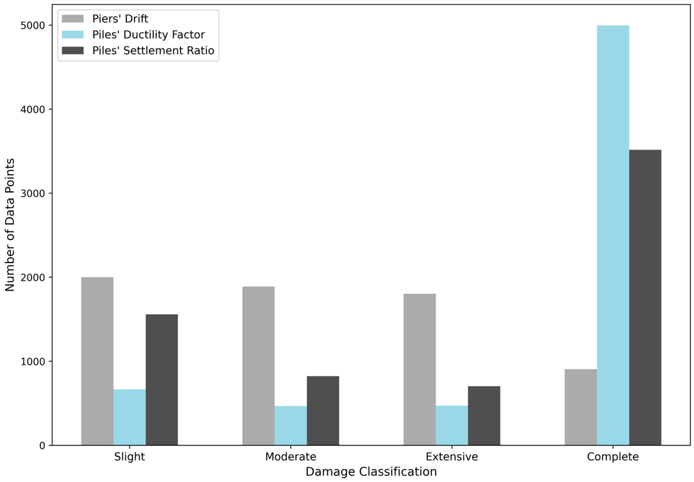
One critical yet frequently overlooked challenge in ML-based seismic assessments is class imbalance within datasets. Due to inherent uncertainties in soil conditions and seismic responses, datasets often exhibit significant imbalances, particularly within severe damage classes. Many studies neglect comprehensive analysis of class imbalance effects, limiting the reliability of minority class predictions. Techniques like Linear and Quadratic Discriminant Analysis and Naïve Bayes are notably affected by class imbalances due to restrictive assumptions on data distributions, as observed in previous studies [26,27].

Furthermore, sophisticated balancing techniques like oversampling and undersampling have shown inconsistent outcomes in ML applications for bridge damage assessments. Although oversampling methods improved predictions for specific metrics such as piers’ drift, they simultaneously increased overfitting risks. Conversely, undersampling frequently resulted in decreased classification accuracy, underscoring the need for more advanced methods capable of adequately representing underlying seismic response complexities.

To the authors’ knowledge, no previous study has specifically explored ML-based classification of seismic damage states for bridges supported by helical pile foundations. Given the unique seismic behavior of helical piles, particularly in cohesive soils, and their growing adoption in engineering practice, addressing this research gap is critical for enhancing rapid damage assessment capabilities and infrastructure resilience.

The present study systematically evaluates various ML algorithms for classifying damage states, specifically targeting piers’ drift, piles’ ductility factors, and piles’ settlement ratios in bridges founded on helical piles. Performance comparisons between advanced algorithms, including CatBoost and Light Gradient Boosting Machine (LightGBM), and traditional classifiers are thoroughly examined. Additionally, the study explicitly investigates the impacts of class imbalance and evaluates the effectiveness of various data-balancing techniques, addressing critical shortcomings in existing literature. Thus, it aims to provide practical insights into ML model selection for seismic damage prediction and support more reliable post-earthquake assessments.

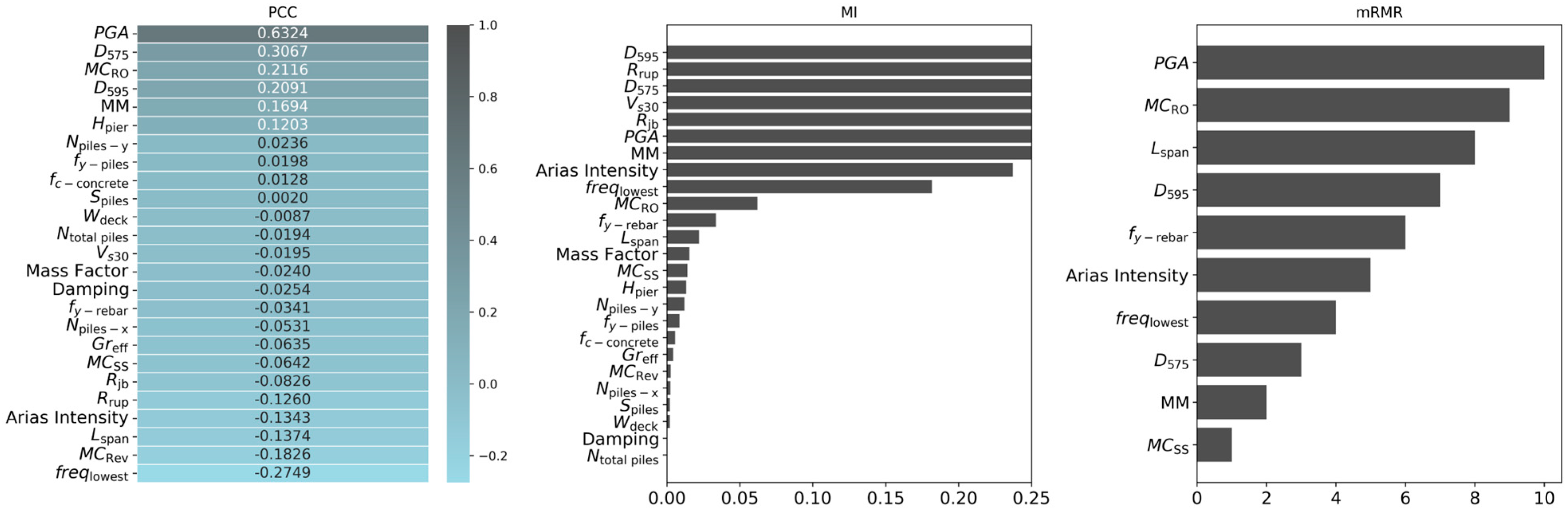
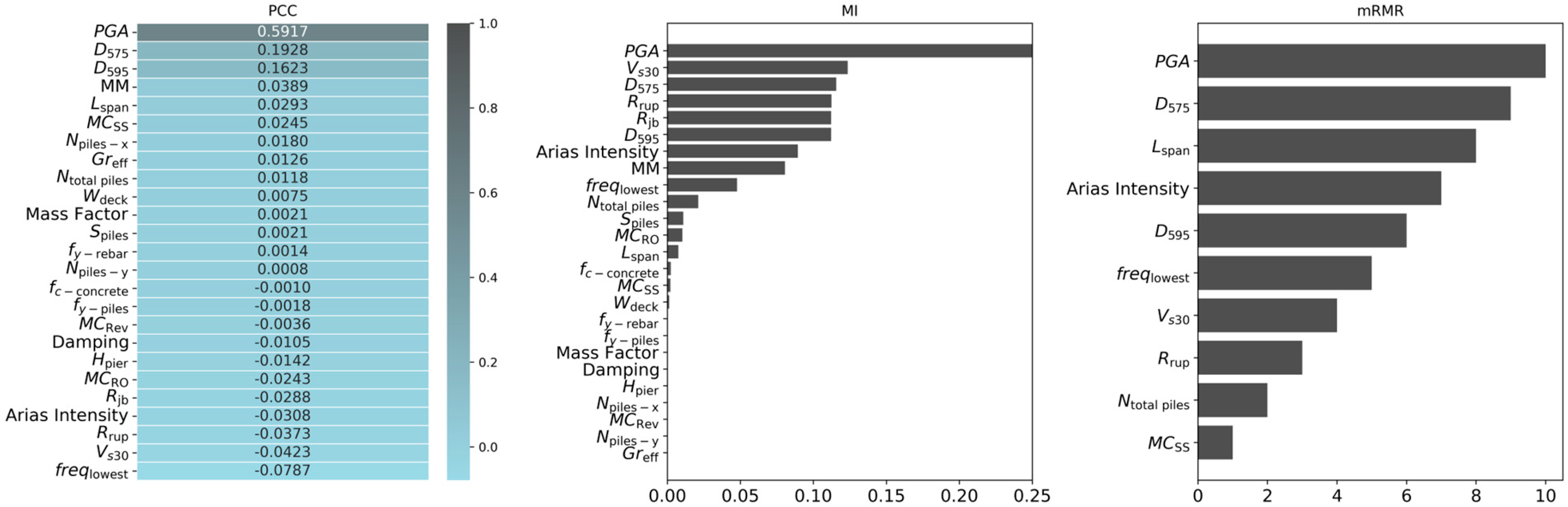
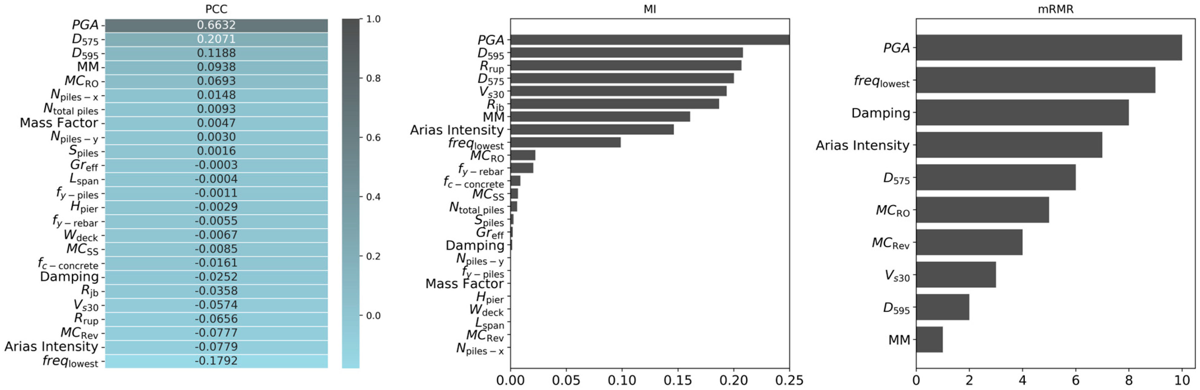
2. Dataset

The study investigates a three-span continuous box girder bridge. OpenSees, an open-source finite element framework, is used to develop the numerical model of the bridge. The validation of the model was previously conducted using shake table test data from [28], as detailed in [29]. A fragility analysis was later performed in [30], where the validated model was modified to better accommodate uncertainties in key parameters, including concrete compressive strength, rebar yield strength, pier height, deck width, span length, pile steel yield strength, mass factor, and damping ratio. To account for these uncertainties, 15 bridge samples were generated using Latin Hypercube Sampling (LHS). While this section provides a summary of the model and ground motion suite, further details can be found in the aforementioned study.

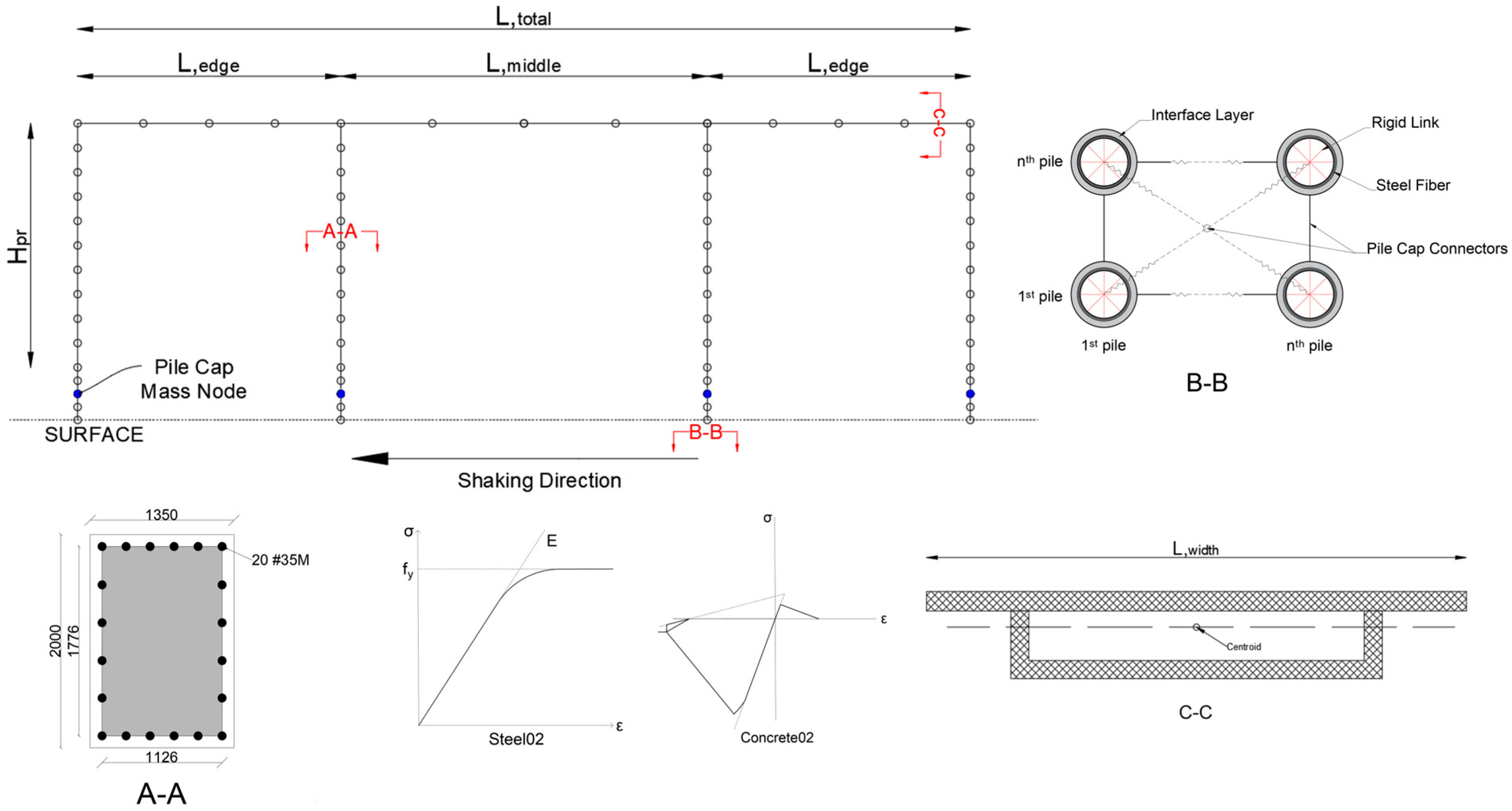
The schematic of the numerical model used in the fragility study is shown in Figure 1. The soil behavior is modeled using 8-node hexahedral brick u-p elements, with the PressureIndependMultiYield material used to simulate cohesive clay. The clay has a mass density of 1.85 $\mathrm{k}\mathrm{g}/\mathrm{c}{\mathrm{m}}^3$, a shear modulus (G) of 78,000 kPa, a bulk modulus of 195,000 kPa, and cohesion of 29.20 kPa. Structural components, including the piles, piers, and deck, are modeled using displacement-based beam–column elements to capture nonlinear flexural behavior. Five Gauss–Legendre integration points are assigned to each element to ensure numerical accuracy. To reduce complexity, pile caps are modeled as elastic beam–column elements.

Each pier is supported by a group of helical piles configured to maintain a minimum factor of safety of 2.60. The piles have a shaft diameter of 610 mm, a wall thickness of 9.40 mm, and two helices, each 1200 mm in diameter, spaced 2.40 m apart. The piles are modeled using displacement beam–column elements, with circular fibers representing the pile shaft. Steel properties are modeled using the Steel02 material, while the helices are represented with ShellMITC4 multilayer shell elements and the J2PlateFibre material. Rigid links are introduced at each pile level to effectively transfer forces between the piles and the surrounding soil. Soil nodes are linked to pile nodes by assigning identical degrees of freedom, and a transition layer is introduced to account for reduced soil stiffness caused by pile installation. The shear and bulk moduli of this transition layer are reduced by 30%.

The piers are also modeled using displacement-based beam–column elements to capture nonlinear seismic response. Each pier tapers from a width of 2 m up to 75% of its height, increasing to 3.50 m at the top. Five fiber sections represent this variation. The core and cover concrete are modeled using the Concrete02 material, and the reinforcement steel is represented with the Steel02 material model. The deck is modeled using elastic beam–column elements, with parameters including cross-sectional area, elastic modulus, shear modulus, and moments of inertia.

A suite of ground motions including 22 earthquake records selected from PEER NGA-West 2 database [31], representing a range of moment magnitudes (5.90 to 7.90), rupture distances (1.70 km to 41.97 km), and predominant frequencies (0.23 to 6.05 Hz), are used in the analysis to account for variability in seismic source and site conditions.

The dataset used in this study originates from 6600 nonlinear time history analyses conducted in the prior fragility study [30]. It serves as the basis for evaluating machine learning algorithms in classifying the seismic damage states of bridge piers and helical piles.

3. Methodology

To prevent data leakage and ensure a robust evaluation, the datasets are divided into 70% of samples for training and 30% for testing before applying any pre-processing steps, using the scikit-learn library [32]. This division is maintained throughout the subsequent data preparation and analysis stages to provide reliable performance estimates for the machine learning algorithms examined in this study. Figure 2 provides a schematic of the workflow and main stages of the analysis.

3.1. Damage Classification

The damage classification task focused on predicting the damage state of three target metrics: piers’ drift, piles’ ductility factor, and piles’ settlement ratio. Following HAZUS guidelines, each target metric is categorized into four damage states: slight, moderate, extensive, and complete.

Drift is selected as the key metric for assessing damage to reinforced concrete piers. This metric measures the relative displacement between the top and bottom of the piers, to capture both elastic and inelastic deformations. Drift is widely used as an engineering demand parameter (EDP) due to its effectiveness in evaluating structural response [33]. The damage states are determined based on drift ratios corresponding to different deformation levels, such as the onset of cover spalling and bar buckling, using empirical relationships proposed by [34,35]. The relationships for determining bar buckling incorporate key parameters such as column depth, axial load, and concrete strength, i.e.,

$${\displaystyle \frac{{\Delta }_{\mathrm{bb}}}{\mathrm{L}}}\left(\%\right)=3.25\mathrm{ }\left(1+{\mathrm{K}}_{{\mathrm{e}}_{bb}}\mathrm{ }{\rho }_{\mathrm{e}\mathrm{f}\mathrm{f}}{\displaystyle \frac{{\mathrm{d}}_{\mathrm{b}}}{\mathrm{D}}}\right)\left(1-{\displaystyle \frac{\mathrm{P}}{{\mathrm{A}}_{\mathrm{g}}\mathrm{ }{\mathrm{f}}_{\mathrm{C}}^{’}}}\right)\left(1+{\displaystyle \frac{\mathrm{L}}{10\mathrm{D}}}\right)$$

(1)

where ${\Delta }_{bb}$ represents the displacement at the onset of bar buckling, $K_{ebb}$ is the transverse reinforcement coefficient (which is 40 for rectangular-reinforced columns), ${\rho }_{eff}$ is the effective confinement ratio, $d_b$ is the diameter of the longitudinal reinforcement bars, P is the axial load, L is the distance from column base to the contraflexure, $A_g$ is gross-area of the cross-section, D is the column depth, and $f_C^{’}$ is the concrete compressive strength.

For slight, moderate, and extensive damage, drift at bar buckling (${\Delta }_{bb}$) = 0.7%, 33%, 67% of ${\Delta }_{bb}$ is used, respectively, following other similar studies [10,36]. For helical piles, two metrics are used: the ductility factor (DF) to quantify flexural damage and the settlement ratio (SR) to evaluate settlement response. The ductility factor (DF), defined as the ratio of ultimate displacement (${∆}_u$) to yield displacement (${∆}_y$) and proposed by [37], is implemented in this study. This factor reflects the ability of piles to endure deformations beyond their initial yielding under lateral loads. Different DF limit states are employed to define the damage states with

$$DF={\displaystyle \frac{∆u}{∆y}}$$

(2)

DF values are adapted from existing recommendations in the literature [10], from slight to complete damage, i.e., DF = 0.6 for slight damage, 1.0 for moderate damage, 1.4 for extensive damage, and 2.0 for complete damage. Furthermore, the settlement ratio (SR) metric is defined using the failure criteria used in previous studies [38,39], which assumes the pile failure occurs when the pile settlement reaches to 10% of shaft diameter (D), with specific thresholds for slight, moderate, extensive, and complete damage adapted from the literature [10]. Specifically, SR = 0.50, 0.75, 1.0, and 1.25 were used for slight, moderate, extensive, and complete damage, respectively.

3.2. Feature Selection

To identify the most informative features for each target variable, three feature selection techniques are applied: Pearson Correlation Coefficient (PCC) [40], Mutual Information (MI) [41], and Minimum Redundancy Maximum Relevance (mRMR) [42]. These methods capture both linear and nonlinear relationships between features and the targets. PCC is used to identify strong linear correlations, particularly relevant for ground motion parameters like Peak Ground Acceleration (PGA), which typically show clear linear trends with damage metrics. To capture more complex dependencies, MI and mRMR are employed. MI quantifies the information shared between variables, while mRMR balances high relevance with low redundancy across features. To avoid multicollinearity, the Variance Inflation Factor (VIF) is also computed.

An initial pool of 24 features is considered, including both ground motion and bridge-specific parameters. Ground motion-related features include PGA, Arias Intensity, Moment Magnitude (MM), and Joyner–Boore Distance ($R_{jb}$), while bridge features cover deck width ($W_{deck}$), span length ($L_{span}$), pier height ($H_{pier}$), concrete compressive strength ($f_{c-concrete}$), rebar yield strength ($f_{y-rebar}$), and the number of piles in both the X and Y directions ($N_{piles-x}$ and $N_{piles-y}$). These features collectively represent the seismic demands and structural characteristics of the bridge. The final selected features vary by target variable and given in

Table 1. Overview of selected features per dataset.

No.	Piers’ Drift	Piles’ D.F. 1	Piles’ S.R. 2
1	PGA 3	PGA 3	PGA 3
2	$R_{jb}$ 4	$R_{jb}$ 4	$R_{jb}$ 4
3	$D_{575}$ 5	$D_{575}$ 5	$D_{575}$ 5
4	Arias Intensity	Arias Intensity	Arias Intensity
5	$f_{c-concrete}$ 6	$f_{y-piles}$ 7	$f_{y-piles}$ 7
6	$f_{y-rebar}$ 8	$N_{piles-x}$ 9	$N_{piles-x}$ 9
7	$H_{pier}$ 10	Damping Ratio	Damping Ratio
8	$L_{span}$ 11	$L_{span}$ 11	$L_{span}$ 11
9	$W_{deck}$ 12	$S_{pile}$ 13	$S_{pile}$ 13

¹ Piles’ Ductility Factor, ² Piles’ Settlement Ratio, ³ Peak Ground Acceleration, ⁴ Joyner–Boore Distance, ⁵ Significant duration between 5% and 75% of Arias Intensity, ⁶ Concrete compressive strength, ⁷ Steel yield strength, ⁸ Rebar yield strength, ⁹ Number of piles in X-direction, ¹⁰ Height of pier, ¹¹ Length of bridge span, ¹² Width of deck, ¹³ Spacing of piles (equal in both directions).

. The PCC, MI, and mRMR scores for each target given in Appendix A.

3.3. Handling Class Imbalance

Classifying the damage state of bridge components under seismic loading inherently results in an imbalanced dataset. This imbalance arises because the damage levels in piers are predominantly influenced by inertial forces associated with seismic excitation, whereas piles experience combined effects from kinematic forces and inertial forces due to the seismic soil–structure interactions. Figure 3 illustrates the distribution of samples across four damage classes considered in this study—slight, moderate, extensive, and complete—for the three target components, highlighting this inherent imbalance.

Addressing class imbalance is essential for developing robust predictive models. Various techniques exist in the literature to mitigate this issue. Oversampling methods, such as the Synthetic Minority Oversampling Technique (SMOTE) [43], create synthetic samples for minority classes to achieve a balanced class distribution. Conversely, undersampling reduces the number of samples in the majority class to match the size of the minority class.

Both oversampling and undersampling techniques are employed to address class imbalance. SMOTE is utilized to generate synthetic samples for the minority classes, enhancing their representation without merely duplicating existing data. Specifically, after applying SMOTE, the class sizes for piers drift, helical pile ductility factor (HP DF), and helical pile settlement ratio (HP SR) are balanced across all damage levels, with each class containing 3834, 6087, and 3666 samples, respectively. This approach ensured that each damage category—slight, moderate, extensive, and complete—is equally represented for each target component.

Likewise, Random Undersampling is applied to reduce the number of majority class samples by randomly selecting a smaller subset. This method achieved balanced class sizes by reducing the sample counts to 905 for piers drift, 852 for HP DF, and 1083 for HP SR across all four damage levels. Although undersampling decreases the overall dataset size, it ensures that all classes are equally represented, thereby minimizing model bias towards majority classes.

To evaluate the effectiveness of these techniques, three versions of the dataset are prepared for each machine learning model: the original imbalanced dataset, a SMOTE-based oversampled dataset, and a randomly undersampled dataset. This approach enables a thorough comparison of classifier performance under different class distribution conditions. Although more advanced resampling methods such as SMOTE variants (e.g., Borderline-SMOTE, SMOTE-Tomek) and ADASYN could potentially improve minority class prediction, they were not considered in this study to limit the scope of the analysis. Future work can incorporate these techniques to investigate the specific advantages of each SMOTE variant and assess their influence on model generalizability and performance.

4. Overview of Machine Learning Techniques

This study employs a variety of machine learning techniques to classify seismic damage in bridge components, comparing traditional and advanced methods. Both linear and nonlinear classifiers are used, along with ensemble and neural network approaches. Traditional methods, such as Discriminant Analysis (DA), K-Nearest Neighbors (KNN), and Naïve Bayes (NB), are combined with Support Vector Machines (SVM), which can model nonlinear boundaries using kernel functions. Ensemble methods, including XGBoost, LightGBM, CatBoost, and ADA Boost, are explored for their ability to enhance prediction accuracy through boosting. Decision Trees (DT) and Random Forests (RF) are implemented to capture complex feature interactions, while Artificial Neural Networks (ANN) are leveraged for their capacity to model nonlinear relationships. These methods are evaluated to determine the most effective model for predicting damage levels under seismic activity. The following sections present a brief overview of each method.

4.1. Discriminant Analysis (DA)

Linear Discriminant Analysis (LDA) is a supervised classification technique that also serves for dimensionality reduction. It projects the feature space onto a lower-dimensional subspace by finding a linear combination of features that maximizes class separation.

LDA achieves this by maximizing the ratio of between-class variance to within-class variance, ensuring distinct class clusters in the transformed space. The primary assumptions of LDA include the following:

• Classes are normally distributed;
• All classes share the same covariance matrix;
• The relationship between features and the target is linear.

On the other hand, Quadratic Discriminant Analysis (QDA) relaxes the equal-covariance assumption of LDA, allowing each class to have its own mean and covariance matrix. This flexibility enables QDA to model more complex, nonlinear boundaries by fitting quadratic surfaces to separate the classes. QDA is particularly effective when class distributions differ significantly in shape or orientation.

4.2. K-Nearest Neighbors (KNN)

The K-Nearest Neighbors (KNN) is a non-parametric, instance-based supervised learning algorithm widely used for classification tasks. Instead of constructing an explicit model, KNN makes predictions directly from the training data by identifying the K-Nearest Neighbors to a new observation [44,45]. To classify damage states, the algorithm begins by selecting a value for k, which determines how many nearby training instances will influence the prediction. The similarity between a new observation ($x_0$) and each training instance ($x_i$) is computed using a chosen distance metric. Common distance measures are given in

Table 2. Common distance metrics.

$d_{Euclidian}\left(x_0,x_i\right)=\sqrt{{\displaystyle \sum _{n=1}^n}{\left(x_0-x_i\right)}^2}$	$d_{Manhattan}\left(x_0,x_i\right)={\displaystyle \sum _{n=1}^n}\left|x_0-x_i\right|$
$d_{Chebyshev}\left(x_0,x_i\right)=\max \left(\left|x_0-x_i\right|\right)$

.

It then calculates the conditional probability of $x_0$ being in a particular damage class (j) as follows:

$$P\left(Y=j|X=x_0\right)={\displaystyle \frac{1}{k}}{\sum }_{i\mathsf{ϵ}{N}_0}I\left(y_i=j\right)$$

(3)

where Y is the damage state, X represents the feature set, $N_0$ contains the indices of the K-Nearest Neighbors, and $I\left(y_i=j\right)$ is an indicator function equal to 1 if neighbor $i$ belongs to class $j$, or 0 otherwise. KNN assumes that instances with similar features are likely to share similar outcomes. While the method is intuitive and easy to implement, its performance depends on feature scaling and is sensitive to noisy or irrelevant features, as it lacks a formal model to generalize from the training data.

4.3. Naïve Bayes (NB)

Naïve Bayes is a probabilistic classification algorithm based on Bayes’ Theorem, which estimates the likelihood of a class given observed features. It computes the posterior probability of each class using prior knowledge and observed data. According to Bayes’ Theorem, the probability of an observation (x) belongs to a damage class (j) is calculated as:

$$P\left(j|x\right)={\displaystyle \frac{P\left(x|j\right)P\left(j\right)}{P\left(x\right)}}$$

(4)

In which, P(j) is the prior probability of the class, $P\left(x|j\right)$ is the likelihood which is the probability of observation x given class j, and $P\left(x\right)$ is the evidence component. The fundamental assumption of the Naïve Bayes classifier is the conditional independence of features. It assumes that each feature contributes independently to the probability, regardless of any possible correlations between features. This simplification is both a strength, making the algorithm fast and easy to implement, and a weakness, as it can lead to less accurate models when features are mutually dependent.

4.4. Support Vector Machines (SVM)

Support Vector Machines (SVM) classifiers are effective in finding decision boundaries for complex datasets, particularly those with high-dimensional features. SVM aims to find an optimal hyperplane that separates data points of different classes [46]. When the data are not linearly separable in the original feature space, SVM applies a kernel transformation to project the input data into a higher-dimensional space, where a linear separator may exist. Commonly used kernel functions are listed in

Table 3. Common kernel functions (a) linear (b) polynomial (c) sigmoid (d) RBF.

(a) $k\left(X_i,X\right)=X_i·X$	(b) $k\left(X_i,X\right)={\left(X_i·X\right)}^e$
(c)$k\left(X_i,X\right)=\tanh \left(\propto X_i^{T}X+r\right)$	(d) $K\left(X_i,X\right)=e^{-\left({\left|X_i-X\right|}^2/2{\sigma }^2\right)}$

.

SVM assumes that the data can be effectively separated in a higher-dimensional space by a hyperplane, implying distinct and separable classes with minimal overlap. However, this assumption may not hold with complex data where class overlap exists. Additionally, SVM can be sensitive to noisy data, as outliers can significantly affect the position of the decision boundary.

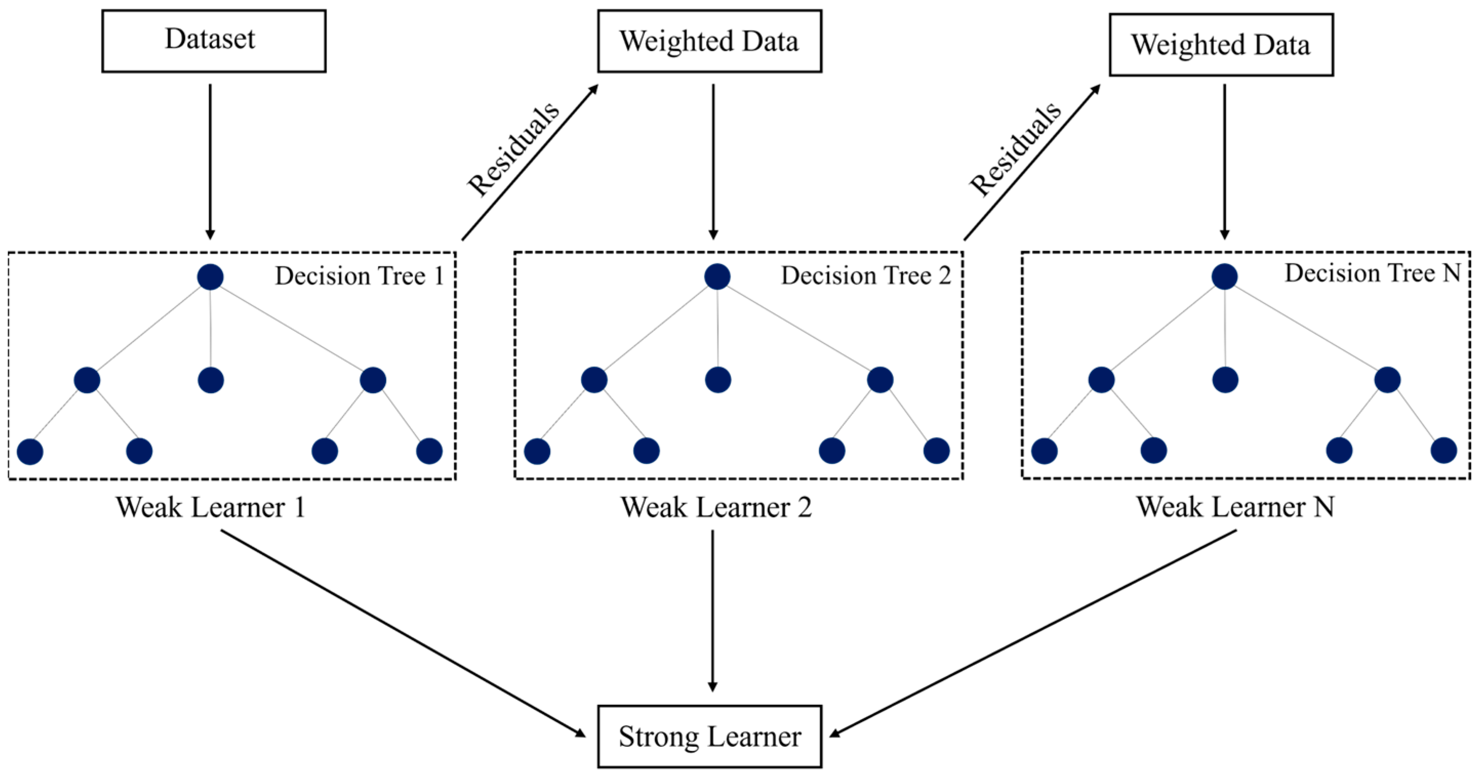
4.5. Boosting Algorithms

Boosting is an ensemble learning technique that combines multiple weak learners—typically shallow decision trees—into a single strong model by sequentially correcting the errors made by previous models. As illustrated in Figure 4, each subsequent model focuses more on the instances misclassified by its predecessor, leading to progressively improved predictions.

This study employs four commonly used boosting algorithms: XGBoost, LightGBM, CatBoost, and AdaBoost. Each of these algorithms follows the core boosting principle but differs in how they handle data structures, optimize learning, and manage categorical variables. The following subsections briefly summarize their key characteristics and differences.

4.5.1. Extreme Gradient Boosting (XGBoost)

XGBoost (Extreme Gradient Boosting) is a scalable implementation of gradient boosting that excels with structured data [47]. It enhances performance through optimization techniques like regularization, tree pruning, and parallel processing. XGBoost employs a second-order Taylor expansion to capture both the gradient and curvature of the loss function, which facilitates faster convergence and improved handling of overfitting. By default, it uses level-wise (depth-wise) tree growth, where trees are expanded level by level.

4.5.2. Light Gradient Boosting (LightGBM)

LightGBM (Light Gradient Boosting Machine) is designed for high efficiency and scalability on large datasets with many features [48]. It introduces a histogram-based algorithm and adopts a leaf-wise (best-first) tree growth strategy, where the leaf with the highest loss reduction potential is split first. This typically leads to deeper, asymmetric trees and often yields higher accuracy compared to the level-wise approach used by XGBoost. Its computational efficiency makes it highly scalable for real-world applications.

4.5.3. Categorical Boosting (CatBoost)

CatBoost is a gradient boosting algorithm optimized for datasets containing categorical variables. It constructs symmetric trees, where splits at each level occur on the same feature, leading to balanced and efficient structures. [49]. To prevent overfitting, CatBoost employs techniques like ordered boosting, which reduces target leakage and minimal data-driven regularization, both of which contribute to better generalization. Its ability to natively handle categorical data without explicit encoding is a key advantage.

4.5.4. Adaptive Boosting (ADABoost)

AdaBoost (Adaptive Boosting), introduced by [50], is one of the earliest boosting algorithms. Unlike gradient-based methods, AdaBoost adjusts the weights of training samples in each iteration, increasing the focus on misclassified instances. Each weak learner, typically a decision stump, is trained sequentially, and this process continues until a specified number of learners is reached or the training error becomes acceptably low. Due to its simplicity and reliance on lightweight base learners, it is computationally efficient and easy to implement.

4.6. Decision Tree (DT)

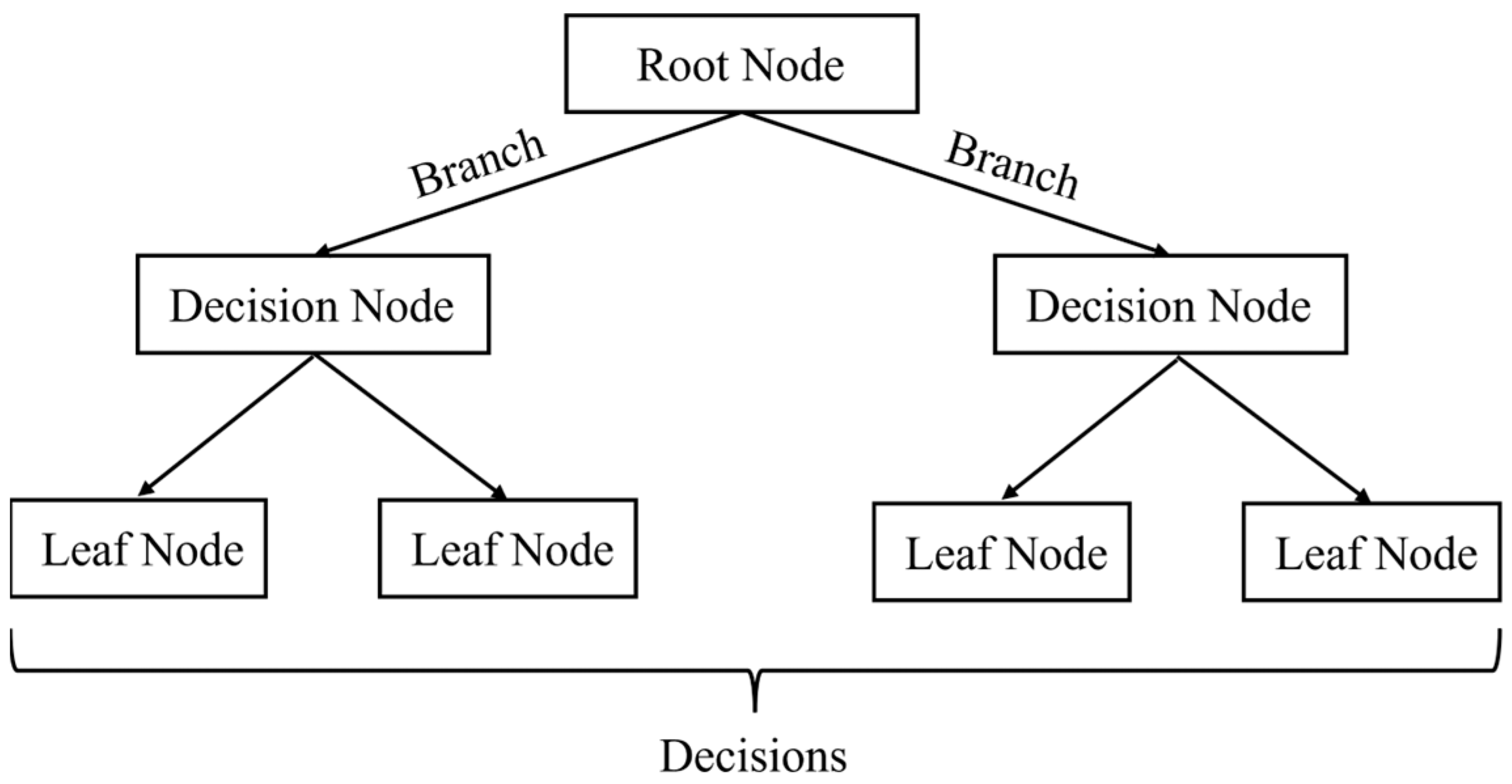
Decision Tree Analysis is a predictive modeling technique that utilizes a tree-like model of decisions and their possible consequences. As illustrated in Figure 5, each internal node represents a test on a feature, each branch corresponds to an outcome of the test, and each leaf node represents a predicted class label. The tree construction begins at a root node and proceeds by recursively splitting the dataset based on criteria such as information gain or Gini impurity, using algorithms like ID3 [51], C4.5 [52], or CART [44]. The process continues until a stopping condition is met, such as a maximum tree depth, a minimum number of samples per leaf, or negligible improvement in impurity reduction.

Decision trees operate under several assumptions: Firstly, each branch from a decision node is expected to cover mutually exclusive subsets of the attribute space, ensuring that no instance can follow more than one path within the tree. Secondly, the branches must collectively account for all possible outcomes of the test, ensuring completeness in the attribute space. Lastly, it is assumed that instances within each leaf node are homogeneous, and that the training data are representative of the population, implying that new data points will adhere to the same statistical distribution.

4.7. Random Forest (RF)

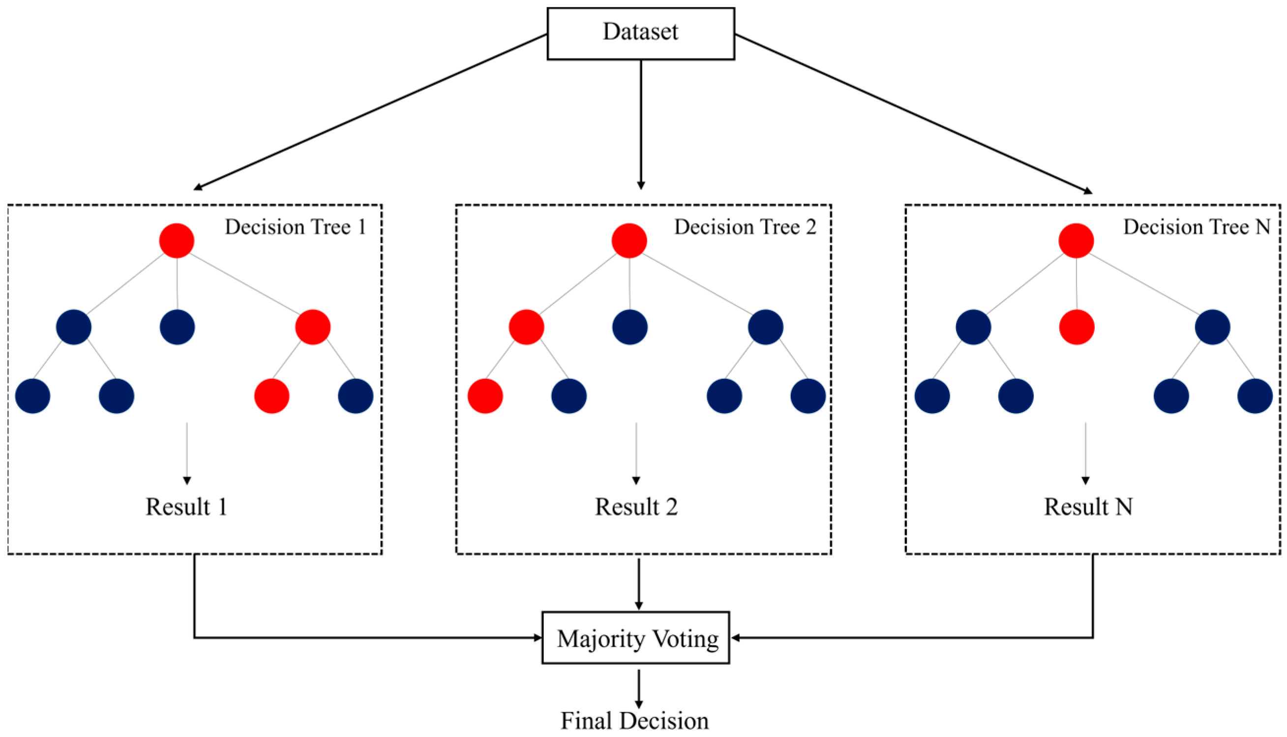
Random Forest is a widely used ensemble classification algorithm that mitigates overfitting by combining the predictions of multiple decision trees. Figure 6 illustrates the concept of the Random Forest algorithm. Each tree in the forest is constructed using a randomly drawn sample from the training set, with replacement, in a process known as bootstrapping. Furthermore, at each split within a tree, a random subset of features is selected as candidates. This additional layer of randomness helps improve model robustness and reduces overfitting.

The algorithm relies on several key assumptions. It assumes that the predictors across trees are independent, which is important for reducing variance through averaging. Each tree is expected to be trained on data drawn from the same distribution, although bootstrapping introduces variation among them. The overall performance typically improves as more trees are added, benefiting from the law of large numbers to produce stable and reliable predictions. While Random Forest is less prone to overfitting compared to single decision trees, it can still exhibit bias in the presence of noisy data or imbalanced class distributions. It may also favor features with many distinct values and can struggle when predictors are highly correlated.

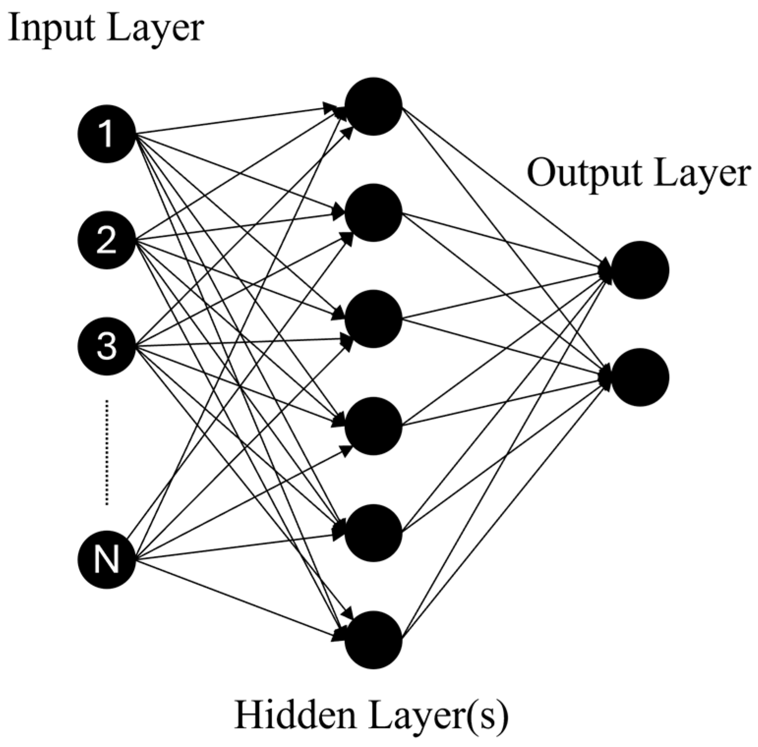
4.8. Artificial Neural Network (ANN)

Artificial Neural Networks (ANNs) are computational models inspired by the structure of biological neural networks. They consist of layers of interconnected nodes, or “neurons”, where each connection is assigned a weight. As shown in Figure 7, data are introduced at the input layer, passes through one or more hidden layers where nonlinear transformations are applied, and finally reaches the output layer, which produces the predicted classification.

In this study, ANNs are used to predict seismic damage metrics, including piers’ drift, helical pile ductility factors, and settlement ratios. Input features such as seismic intensity measures and structural parameters are fed into the network. Each neuron in the hidden layers computes a weighted sum of its inputs and applies a nonlinear activation function (e.g., Sigmoid, Tanh, or ReLU) to introduce nonlinearity and model complex relationships. The model is trained using backpropagation, an iterative optimization process that adjusts the weights by minimizing the difference between predicted and actual outputs. This is achieved by computing the gradient of a loss function and updating the weights to reduce prediction error.

While ANNs are powerful tools for learning patterns in complex, high-dimensional datasets, they are often regarded as black-box models due to their lack of interpretability. Understanding how inputs influence outputs can be challenging. Moreover, the performance of ANNs is highly sensitive to architectural choices, such as the number of layers and neurons. Determining an effective network structure typically requires extensive experimentation and tuning.

5. Results and Discussions

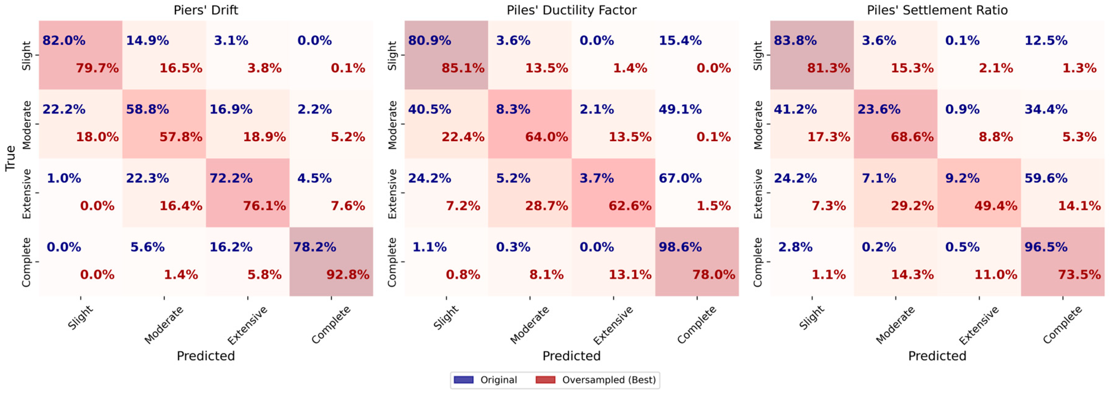
The performance of each machine learning algorithm is evaluated using macro-averaged accuracy, precision, recall, and F1-score metrics, along with their corresponding normalized confusion matrices. To facilitate comparison, confusion matrices are plotted for each target variable, piers’ drift, helical piles’ ductility factor (HP DF), and settlement ratio (HP SR), and arranged in three columns. Each subsection analyzes a specific algorithm, highlighting its strengths and weaknesses in classifying damage states. A final comparative discussion summarizes key differences in model performance across the three targets under both imbalanced and balanced dataset conditions.

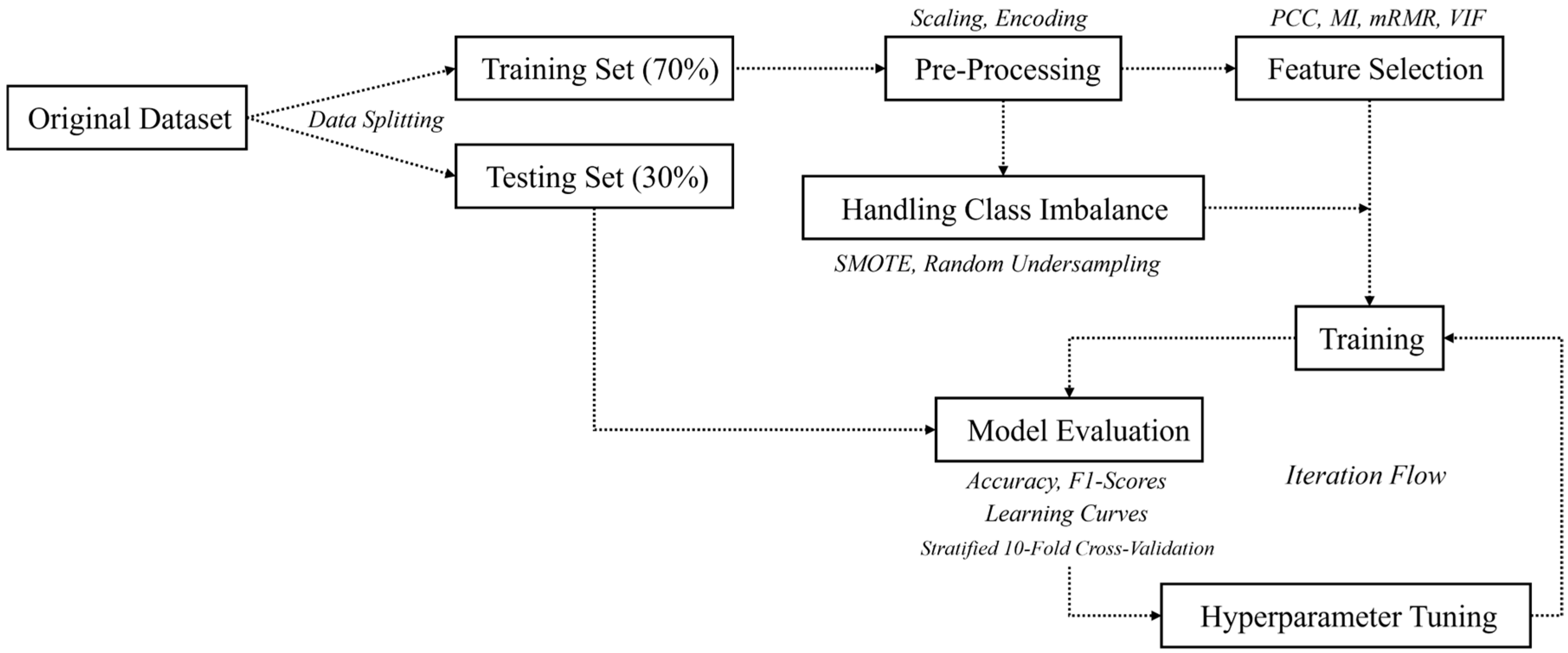
All machine learning tasks were implemented in Python (version 3.11.5). For all models except the Artificial Neural Network (ANN), scikit-learn [32] (version 1.6.1) was used to generate confusion matrices, classification reports, learning curves, conduct stratified k-fold cross-validation, and perform hyperparameter tuning via grid search. The ANN model was developed and trained using TensorFlow [53] (version 2.18.0).

5.1. Discriminant Analysis (DA)

Both Linear Discriminant Analysis (LDA) and Quadratic Discriminant Analysis (QDA) are tuned using grid search with 10-fold stratified cross-validation. For LDA, the hyperparameters explored include the solver type (Least Squares, Eigenvalue Decomposition), shrinkage values ranging from none to 1.0, and the number of components (1 to 3). For QDA, regularization values are varied from 0.0 to 1.0 in increments of 0.05.

Figure 8 presents the results for LDA across the three target variables. For piers’ drift, LDA achieves an F1-score of 0.54 on the original imbalanced dataset, with better precision observed in the slight and complete damage classes. However, it performs poorly on moderate and extensive classes, reflecting LDA’s sensitivity to class imbalance. Applying oversampling improves the overall F1-score slightly to 0.56, but moderate damage remains underrepresented with an F1-score of 0.33. Undersampling produces a similar overall score (0.56) but does not address the class imbalance issue effectively. For HP DF target, LDA performs better on the original dataset (F1-score 0.76) but struggles with minority classes. Oversampling reduces performance (F1-score 0.49), which suggests synthetic data does not align well with LDA’s assumptions. Undersampling further decreases performance (F1-score 0.45), indicating LDA handles the original imbalanced data best. For HP SR target, LDA achieves an F1-score of 0.60 on the original dataset, with complete damage class performing best. Oversampling and undersampling reduce performance to F1-scores of 0.45 and 0.44, respectively, which indicates limited benefit from resampling.

Similarly, Figure 9 presents the classification results obtained using QDA. For the piers’ drift target, QDA exhibits a performance trend similar to LDA. The original dataset yields an F1-score of 0.58, with higher precision for the slight and complete damage classes, while performance drops for the moderate and extensive classes. Oversampling improves the overall F1-score to 0.61, with noticeable gains in the moderate class. Undersampling results in an F1-score of 0.59, comparable to the original data. For HP DF, QDA performs well on the original dataset (F1-score 0.77) but struggles with minority classes. Oversampling and undersampling reduce the F1-scores to 0.51 and 0.44, respectively, with limited improvement for minority classes. For HP SR, QDA achieves an F1-score of 0.65 on the original dataset, with strong performance for complete damage but low precision for minority classes. Oversampling and undersampling lead to F1-scores of 0.48 and 0.44, respectively, showing limited gains from resampling.

Overall, both LDA and QDA face limitations when dealing with imbalanced datasets, particularly for moderate and extensive damage classes. While LDA shows minor gains from oversampling for piers drift, and QDA slightly benefits for the same target; neither model demonstrates consistent improvement across all targets. These findings indicate that resampling alone does not adequately resolve class imbalance issues for discriminant analysis models.

5.2. K-Nearest Neighbors (KNN)

The KNN model is optimized using grid search across a range of hyperparameters, including the number of neighbors, distance metrics, and weighting functions. As shown in Figure 10, KNN performs well in terms of accuracy and F1-scores. However, several issues suggest it may not be suitable for this complex dataset.

KNN’s performance is significantly affected by the complexity and dimensionality of the dataset. Its instance-based nature makes it prone to overfitting when feature interactions are complex or when noise is present. These issues are illustrated in the learning curves in Figure 11. For all three targets, piers’ drift, HP DF, and HP SR, the training scores remain close to 1.0, while the cross-validation scores improve only marginally with increased training data. This persistent gap between training and validation performance is a clear indicator of overfitting.

In the oversampled datasets, overfitting is somewhat reduced, as evidenced by the cross-validation curves approaching the training curves. However, the gap never fully closes, suggesting that even with balanced data, the model struggles to generalize. In undersampled datasets, the problem is more pronounced: reduced sample size increases sensitivity to noise and outliers, leading to approximately a 10% drop in both accuracy and F1-scores across all target variables.

While KNN achieves high performance metrics under certain conditions, these results may reflect memorization rather than learning. Its poor generalization, high variance, and sensitivity to class imbalance and noise limit its suitability for this complex seismic damage classification task.

5.3. Naïve Bayes (NB)

Gaussian Naïve Bayes was applied to the seismic damage classification dataset, yielding mixed results as shown in Figure 12. While the overall performance metrics (i.e., accuracy and F1-score) are reasonable across different datasets, the model’s core assumption that features are conditionally independent limits its effectiveness in this context. The algorithm’s strong assumption of feature independence often leads to suboptimal performance in complex, high-dimensional datasets, where feature interactions are critical in defining the target classes. The results across the different datasets highlight some strengths and weaknesses of the model.

For the piers’ drift target, the model achieves an accuracy of 0.58 and F1-score of 0.56 on the original dataset. Oversampling slightly improves performance (accuracy: 0.61, F1-score: 0.59), while undersampling yields similar results (accuracy: 0.58, F1-score: 0.57). As shown in Figure 13, the training and cross-validation scores remain relatively close, but improvements with more training data are limited, which is an indication that the model does not benefit from increased sample size due to its simplistic structure.

For piles’ ductility factor (HP DF), the model performs reasonably well on the original dataset (accuracy: 0.82, F1-score: 0.76). However, performance deteriorates sharply with oversampling (accuracy: 0.46, F1-score: 0.43) and undersampling (accuracy: 0.44, F1-score: 0.40). The learning curves support this trend, showing flat validation scores regardless of increased training data, reflecting poor adaptability to data complexity and noise.

For piles’ settlement ratio (HP SR), Naïve Bayes achieves 0.70 accuracy and 0.63 F1-score on the original dataset. Again, oversampling reduces performance (accuracy: 0.48, F1-score: 0.45), with similar declines seen in the undersampled data (accuracy: 0.46, F1-score: 0.43). The corresponding learning curves indicate a drop in training performance with increased data, highlighting the model’s difficulty in generalization.

Overall, Naïve Bayes performs better on the original datasets, particularly for HP DF, but struggles with resampled data due to its restrictive assumptions. Although oversampling offers marginal gains for some targets, the model fails to capture complex feature dependencies inherent in seismic damage patterns. The learning curves further confirm that Naïve Bayes cannot leverage larger datasets effectively, emphasizing the need for more advanced models in this setting.

5.4. Support Vector Machines (SVM)

The SVM model, optimized through grid search using hyperparameters (C, kernel, and gamma), demonstrates relatively strong performance across the seismic damage classification tasks. Despite the inherent complexity and imbalance in the datasets, SVM achieves notable accuracy and F1-scores, making it a competitive model. However, a closer look into the confusion matrices displayed in Figure 14 and the learning curves presented in Figure 15 reveals important insights about its strengths and limitations.

For piers’ drift target, SVM achieves an accuracy and F1-score of 0.72 on the original dataset. It classifies slight and complete damage states effectively but struggles with moderate and extensive classes. Oversampling improves performance (accuracy: 0.77, F1-score: 0.76), while undersampling yields comparable results to the original dataset (accuracy and F1-score: 0.72). The learning curves shown in Figure 15 indicate improved cross-validation scores with increasing data, suggesting that SVM benefits from larger sample sizes.

For piles’ ductility factor (HP DF), SVM achieved an accuracy of 0.83 and an F1-score of 0.77 on the original dataset. The confusion matrix highlights strong performance in classifying the complete class, while performance dropped for moderate and extensive classes. Oversampling reduced both accuracy (0.70) and F1-score (0.71), indicating challenges with the added complexity of the data. However, it significantly improved the accuracy of the minority classes. This is also reflected in the learning curves, where the gap between training and validation scores narrows as more samples are added. In the undersampled dataset, accuracy drops further to 0.48 and the F1-score to 0.43, suggesting the model struggles with the reduced dataset size.

For piles’ settlement ratio (HP SR), SVM achieves an accuracy of 0.73 and an F1-score of 0.66 on the original dataset, with strong performance in slight and complete classes but difficulties with moderate and extensive cases (minority classes). Oversampling decreases both metrics (accuracy: 0.64, F1-score: 0.64), and undersampling results in further performance degradation (accuracy: 0.51, F1-score: 0.49). The persistent gap between training and validation curves indicates limited benefit from additional data and a sensitivity to noise and class overlap.

Overall, SVM is effective at handling the nonlinear patterns of seismic damage classification, especially on original datasets. However, it is sensitive to both data imbalance and dimensionality. Oversampling may introduce noise, leading to overfitting, while undersampling can result in underfitting and reduced generalization. These outcomes emphasize the importance of balancing data quality and model complexity when applying SVM to imbalanced, high-dimensional problems.

5.5. Boosting Algorithms

5.5.1. Extreme Gradient Boosting (XGBoost)

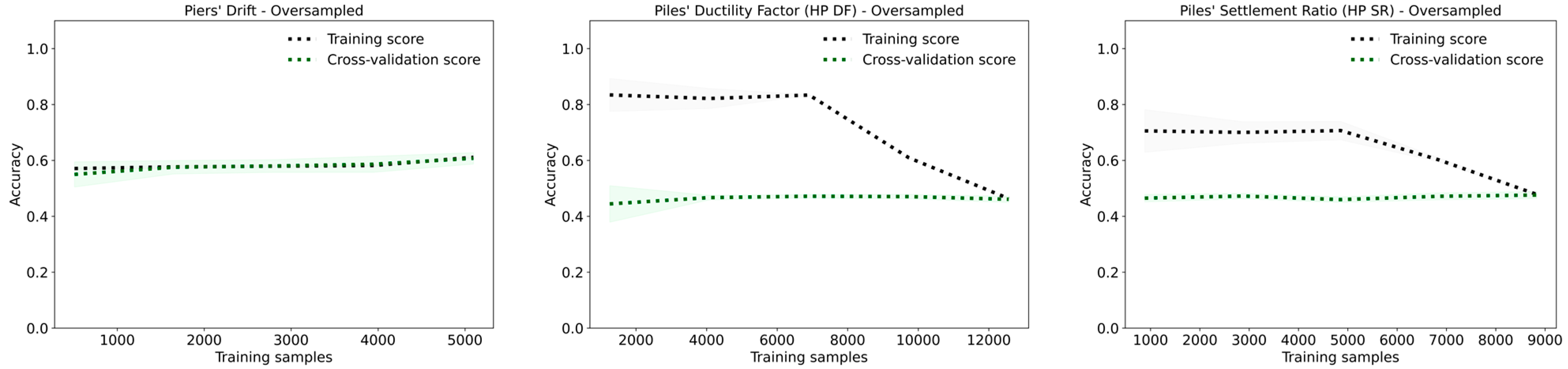
As shown in Figure 16, the XGBoost model exhibits consistent trends across all datasets. For piers’ drift, the original dataset yields an accuracy and F1-score of 0.80. The oversampled dataset slightly improves overall performance, achieving accuracy and F1-score of 0.81, while the undersampled dataset results in a comparable accuracy and F1-score of 0.79. These results indicate that oversampling enhances prediction accuracy, particularly for the minority classes, without adversely affecting the model’s overall performance.

For the piles’ ductility factor (HP DF), the original dataset achieves the highest accuracy at 0.89. In comparison, the oversampled and undersampled datasets show slightly lower accuracies of 0.82 and 0.78, respectively. This trend reflects the influence of data balancing on predictive accuracy, especially for underrepresented classes. While oversampling improves classification in minority categories, it introduces a minor trade-off in overall precision.

For piles’ settlement ratio (HP SR), the model achieves an accuracy of 0.81 and an F1-score of 0.76 on the original dataset. Performance declines with oversampling and undersampling, with both accuracy and F1-score dropping to 0.78 and 0.75, respectively. These results suggest that HP SR is a more challenging target for XGBoost. Although class imbalance is addressed through resampling, neither method fully resolves the difficulty in improving predictive accuracy for this variable.

The learning curves exhibited in Figure 17 provide further insights into model performance. For the oversampled piers’ drift dataset, both the training and cross-validation scores converge as more samples are added, indicating reduced overfitting and improved generalization. For the oversampled HP DF, the training score starts high and gradually decreases, while the cross-validation score improves, indicating that the model is learning from a more diverse dataset, which helps in reducing overfitting. In contrast, for the oversampled HP SR, the training score is consistently higher than the cross-validation score, and there is a slight decline in the training score as more samples are added, suggesting that overfitting is gradually being mitigated but still present.

For the original datasets, the training scores are initially high, with signs of overfitting, as indicated by the gap between the training and cross-validation scores. As the number of samples increases, the gap narrows, showing that the model becomes better at generalizing. The HP SR learning curve particularly shows a stable performance across increasing samples, with the training and cross-validation scores closely aligning, indicating no significant signs of overfitting in the original datasets.

5.5.2. Light Gradient Boosting (LightGBM)

The confusion matrices from the LightGBM models are presented in Figure 18, and the corresponding learning curves are shown in Figure 19. A grid search technique is used to optimize hyperparameters, including learning rate, maximum depth, number of estimators, number of leaves, minimum child samples, minimum split gain, and regularization terms (α and λ). Model evaluation is conducted via stratified K-fold cross-validation.

For piers’ drift target, the original dataset achieves an accuracy and F1-score of 0.93, while the oversampled dataset improves slightly to 0.94. The undersampled dataset yields an accuracy and F1-score of 0.92. Training scores initially start slightly lower and stabilize after around 1500 samples, eventually reaching near-perfect values. Cross-validation scores gradually improve and converge to the reported metrics. However, the consistently perfect training score (1.0) indicates potential overfitting, particularly in the oversampled dataset. Although cross-validation performance improves with more data, the model’s ability to memorize noise and minor fluctuations in the input contributes to this overfitting. Nonetheless, the narrowing gap between training and validation curves reflects improved generalization as more samples are introduced.

Similar trends are observed for helical pile ductility factor (HP DF) and helical pile settlement ratio (HP SR). For HP DF, the original dataset achieves an accuracy and F1-score of 0.96, while the oversampled and undersampled datasets yield 0.94 and 0.88, respectively. For HP SR, the original and oversampled datasets both result in 0.93 accuracy and F1-score, while the undersampled version produces 0.88 for both metrics.

In the oversampled datasets for HP DF and HP SR, training scores remain near-perfect throughout most of the training process, and the gap with cross-validation scores persists until the final training samples. This behavior again suggests overfitting due to the model’s tendency to learn fine-grained, potentially uninformative patterns introduced by synthetic data. In contrast, the original datasets show convergence after approximately 1500 samples, indicating improved generalization. For the oversampled sets, training scores begin to decrease slightly after 8000 samples, likely reflecting the increased data variety introduced through resampling.

5.5.3. Categorical Boosting (CatBoost)

The CatBoost classifier is used for each dataset (original, oversampled, and undersampled) to assess model performance for piers’ drift, piles’ ductility factor, and piles’ settlement ratio. The parameter grid for hyperparameter tuning includes the number of iterations, learning rate, tree depth, L2 regularization, random strength, subsample rate, and bootstrap type. The training and cross-validation results for each case are summarized based on classification metrics shown in Figure 20 and learning curves presented in Figure 21.

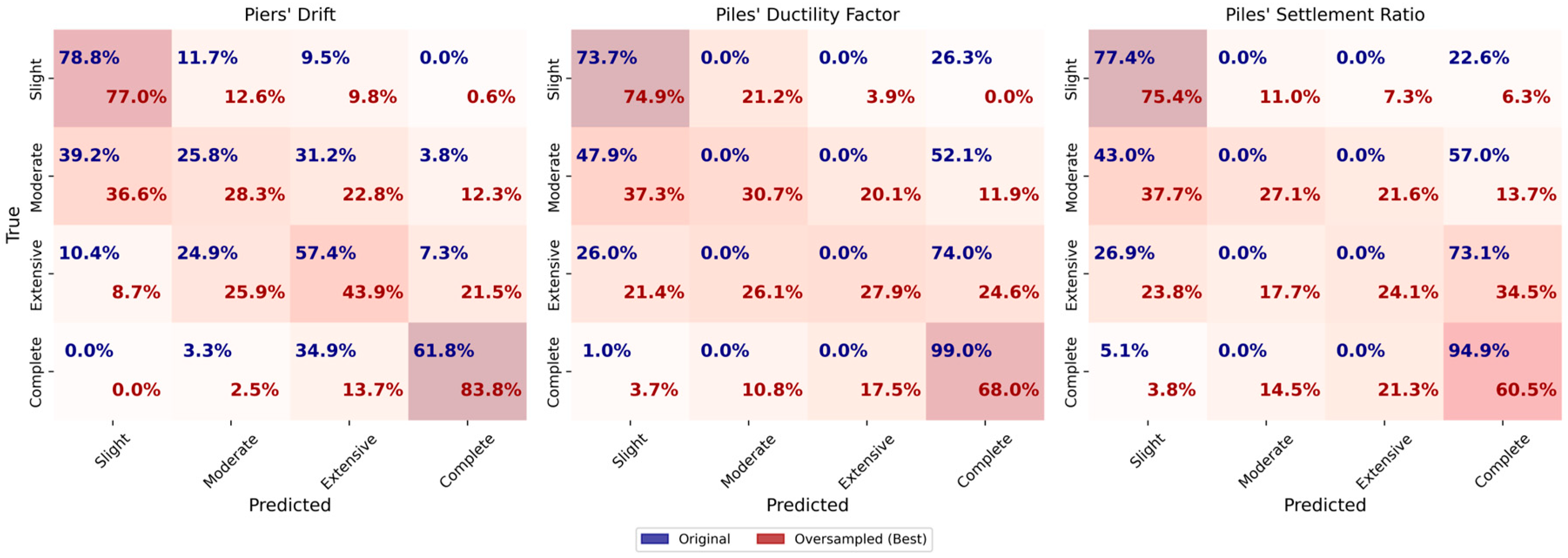
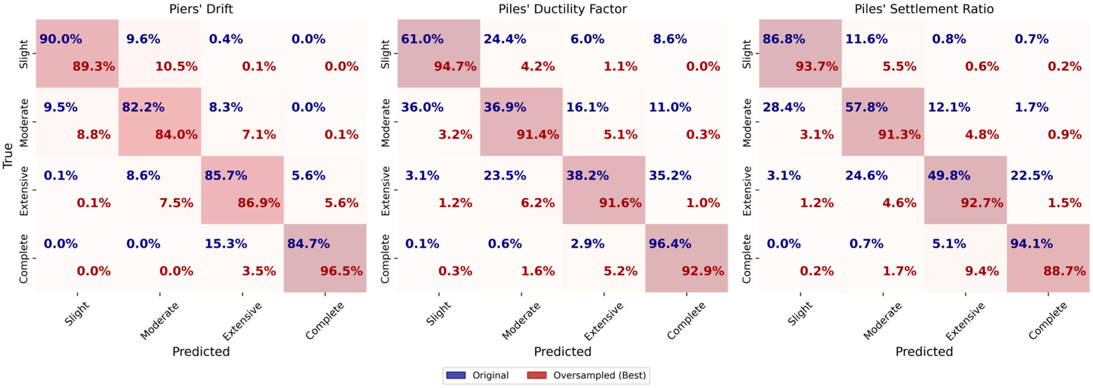
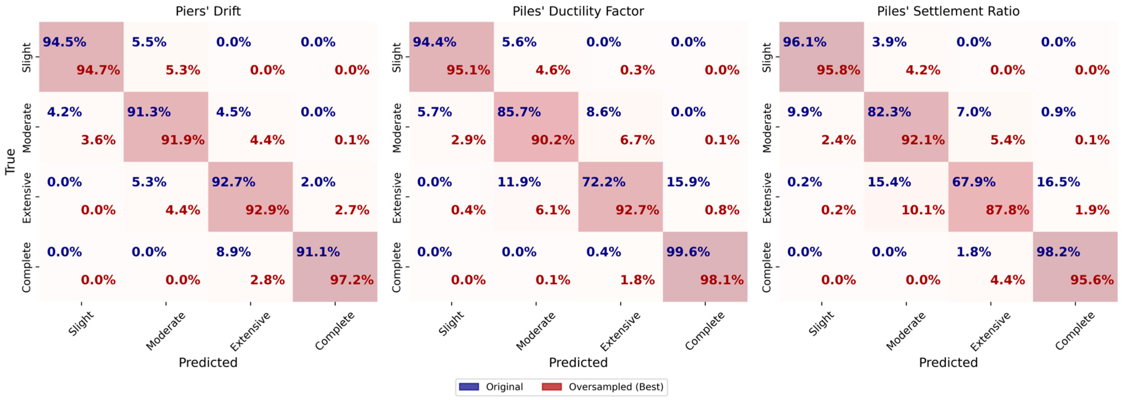
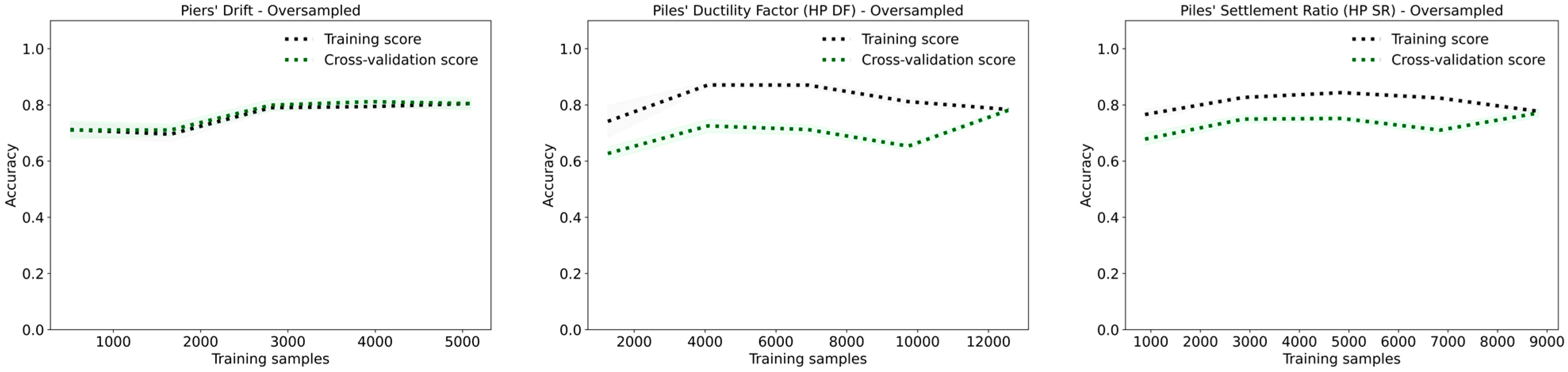
For piers’ drift, the CatBoost model performed well for the original dataset, achieving an accuracy and F1-score of 0.93. The oversampled dataset shows slightly better performance with an accuracy and F1-score of 0.94, suggesting that oversampling helps mitigate class imbalance and improve generalization. The undersampled dataset shows reduced performance, with an accuracy and F1-score of 0.92.

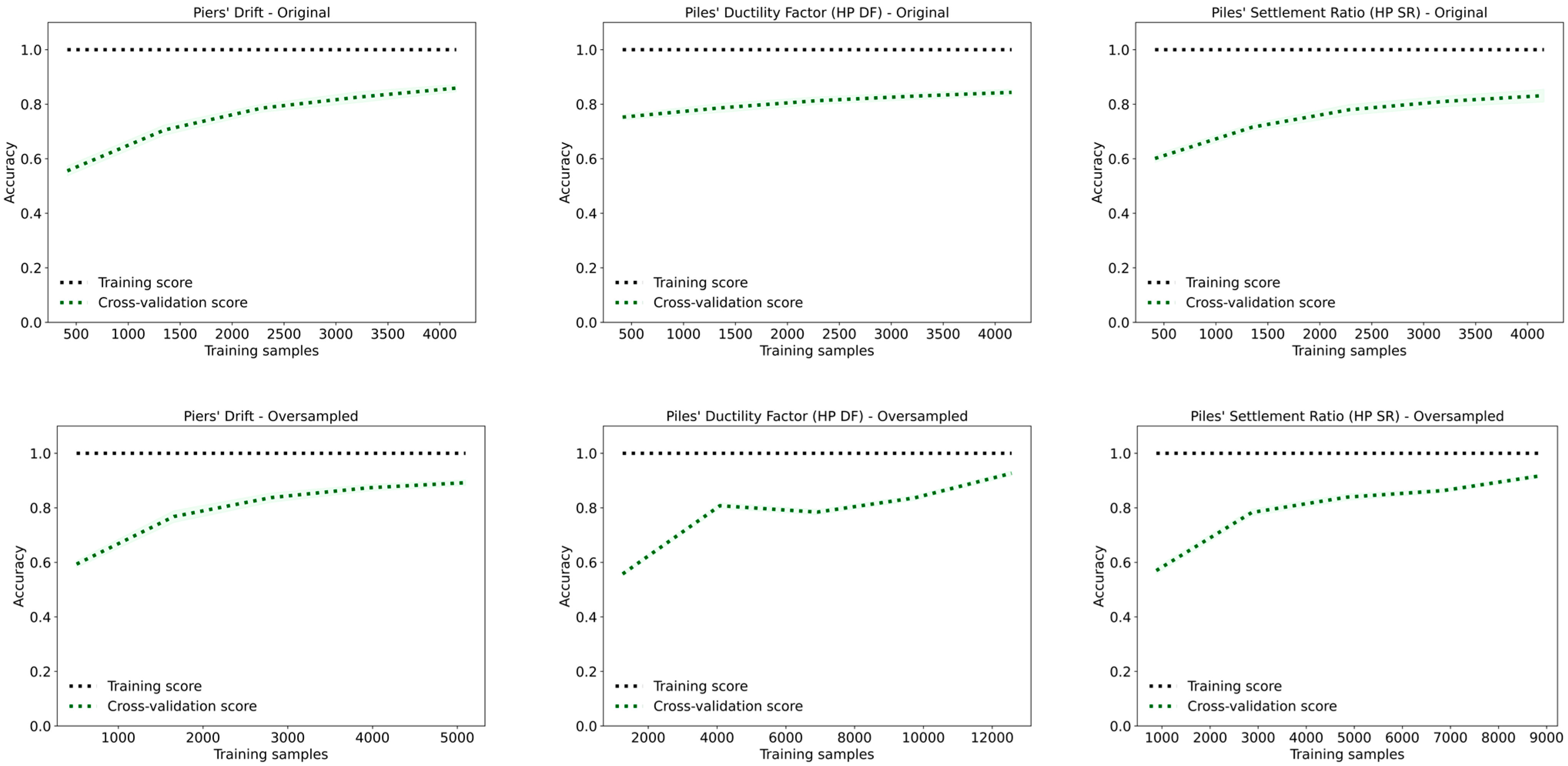
The learning curves presented in Figure 21 indicate that the cross-validation score for the oversampled dataset gradually converges towards the training score, while the original dataset has a minor gap, indicating some overfitting. The undersampled dataset shows a larger gap between training and validation scores, reflecting the effect of limited data on model generalization.

For piles’ ductility factor (HP DF), the original dataset achieves an accuracy and F1-score of 0.96. The oversampled dataset performs slightly worse, with an accuracy and F1-score of 0.93, while the undersampled dataset has the lowest performance, with an accuracy and F1-score of 0.89. The learning curves for the oversampled dataset exhibit a consistent high training score, while the cross-validation score initially decreases, then improves gradually. The original dataset shows a similar trend but with a narrower gap, suggesting better generalization compared to the oversampled dataset. The undersampled dataset has a persistent gap between training and cross-validation scores, highlighting the limitations of reduced data.

For piles’ settlement ratio (HP SR), the original dataset achieves an accuracy and F1-score of 0.92. The oversampled dataset has a slightly lower accuracy and F1-score of 0.91, while the undersampled dataset performed the worst, with an accuracy and F1-score of 0.88. The learning curves for both the original and oversampled datasets show high training scores close to 1.0, with the cross-validation score gradually improving as more samples are added. The oversampled dataset shows a slightly narrower gap between training and validation scores compared to the original dataset, indicating improved generalization. However, the persistent gap suggests overfitting remained an issue. The undersampled dataset shows a larger gap between training and cross-validation scores, again reflecting the impact of limited data on model performance.

5.5.4. Adaptive Boosting (ADABoost)

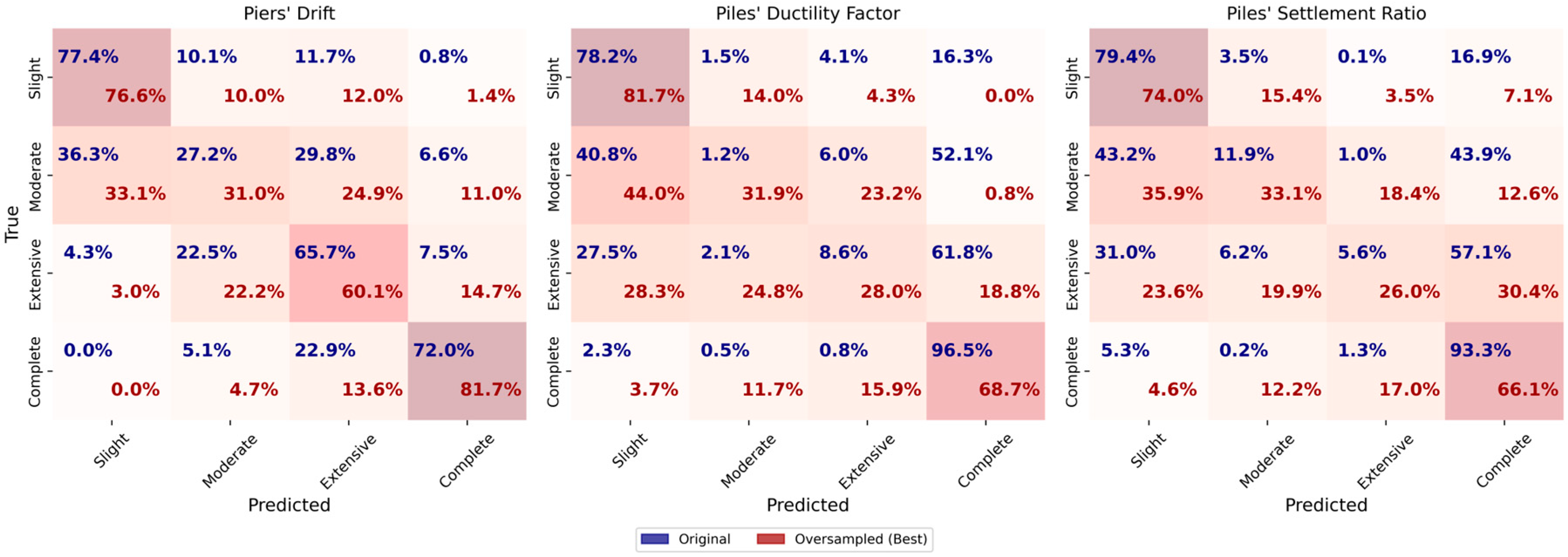
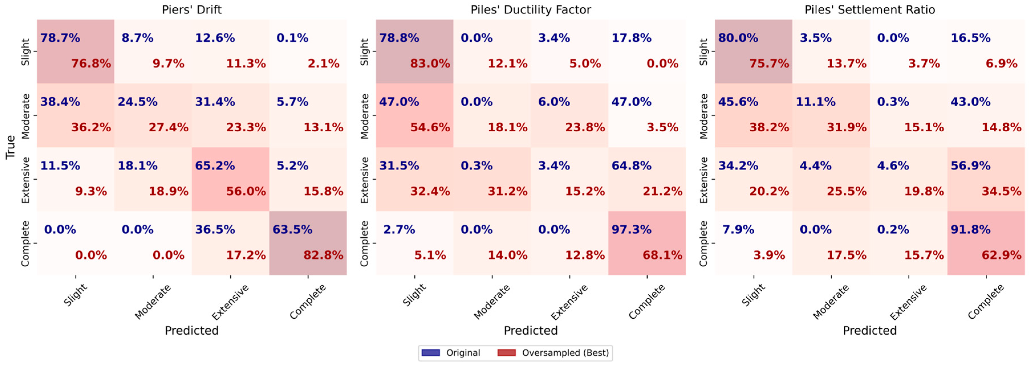
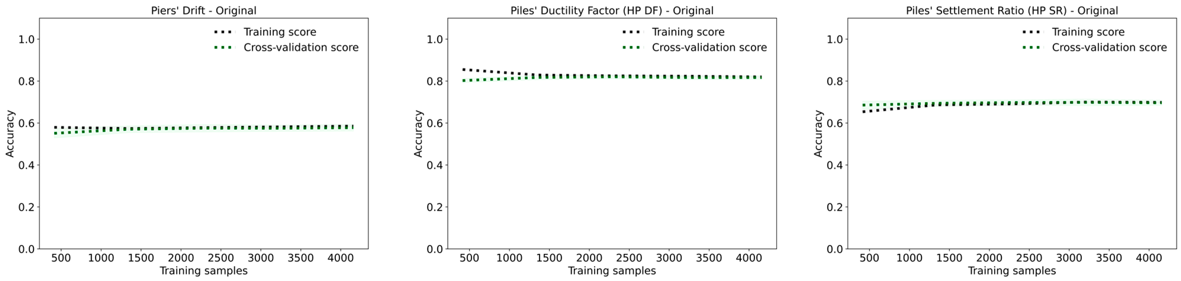
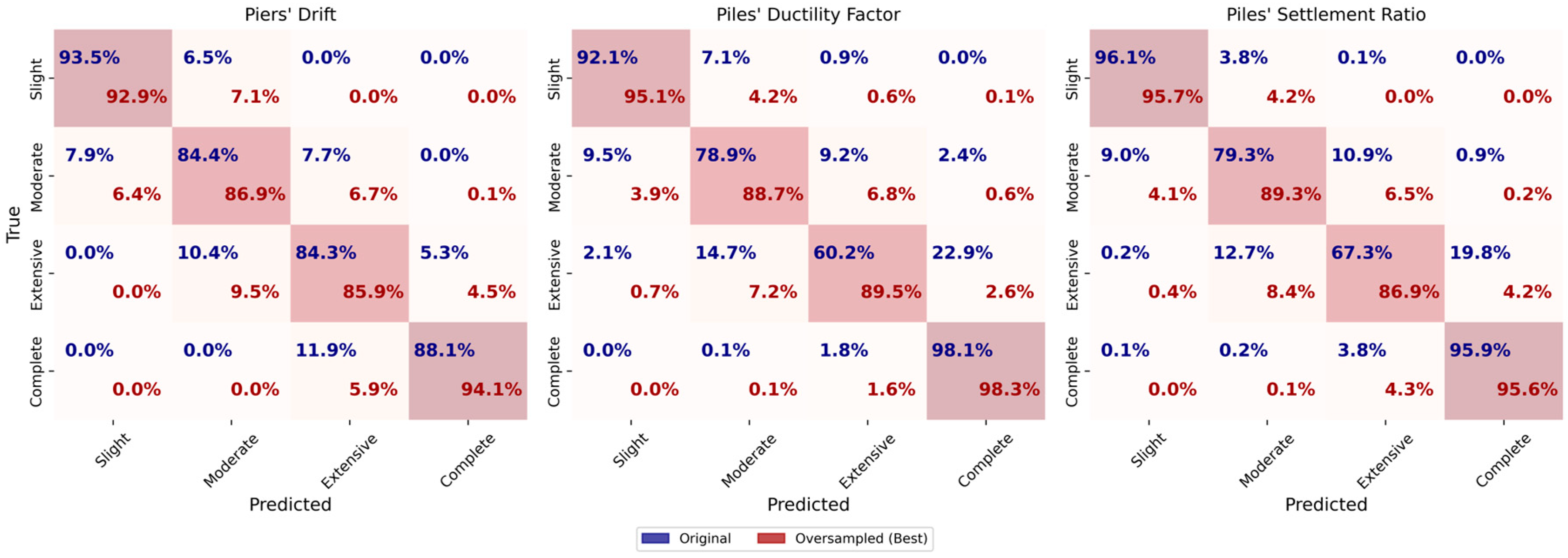
Figure 22 shows the confusion matrices obtained from ADABoost models. For piers’ drift, HP DF, and HP SR, the ADABoost model with 200 estimators and a learning rate of 1.0 performs best across all datasets. The model is optimized using a GridSearchCV approach, where a grid search is conducted to determine the optimal hyperparameters, including the number of estimators and the learning rate. Stratified K-Fold cross-validation with 10 splits is used to ensure robust hyperparameter tuning.

In the original dataset, the accuracy and F1-score for piers’ drift is 0.79. The oversampled dataset achieves the highest accuracy and F1-score, both at 0.80. The undersampled dataset also achieves an accuracy and F1-score of 0.80, indicating consistent performance across sampling methods. The learning curves for piers’ drift show good generalization in both the original and oversampled datasets, with the gap between training and cross-validation scores becoming negligible as more samples are added, as seen in Figure 23. This indicates that the model learned effectively without overfitting.

For HP DF, the original dataset achieves an accuracy and F1-score of 0.87, which is the highest among the datasets, which demonstrate strong performance and generalization. In the oversampled dataset, the accuracy and F1-score are both 0.78, but significant overfitting is observed. This is indicated by the training score initially increasing, then stabilizing, and finally decreasing, while the gap between the training and cross-validation scores continued to widen. The undersampled dataset has lower values, with an accuracy and F1-score of 0.72. The learning curves for HP DF in the oversampled dataset show a persistent gap between the training and cross-validation scores, indicating potential overfitting.

For HP SR, the original dataset perform well, with an accuracy and F1-score of 0.83. In the oversampled dataset (F1-score 0.78), significant overfitting is again observed; the training score initially increases, then stabilizes and finally decreases, while the gap between the training and cross-validation scores widens. The undersampled dataset show an accuracy and F1-score of 0.75. Similar observations are made in the training curves as HP DF but with less overfit.

5.6. Decision Tree (DT)

The Decision Tree models are optimized using a grid search exploring key hyperparameters, including split criterion, maximum tree depth, minimum samples per split, and per leaf. The split criterion, either ‘gini’ or ‘entropy’, favored ‘entropy’ for most datasets, indicating that information gain is more effective. Maximum tree depth is left unconstrained to fully capture complex feature relationships. Minimum samples per split and per leaf are set to 20 and 10, respectively, balancing overfitting prevention and model flexibility.

Figure 24 presents the confusion matrices obtained from decision tree models. The oversampled dataset achieves the best performance for piers’ drift with an accuracy and F1-score of 0.90. The accuracy and F1-score are both 0.88 and 0.85 for the original dataset and undersampled dataset, respectively. The oversampled dataset shows the best results due to more balanced data, leading to improved model generalization.

The learning curves displayed in Figure 25 show consistent performance with minimal variance, indicating effective generalization. As more samples are added, the curves follow the same upward trend with a very slight slope, showing an increase in accuracy. The gap between the training and validation curves decrease for the oversampled dataset, indicating reduced overfitting.

For HP DF, both the original and oversampled datasets result in accuracy and F1-score of 0.93, indicating consistent and strong performance across data conditions. The undersampled dataset yields lower performance, with an accuracy and F1-score of 0.84, likely due to reduced training data. The learning curves show improvement as more samples are introduced, and for the original dataset, the model generalizes well. However, the oversampled dataset shows signs of overfitting, as evidenced by a growing gap between training and validation scores.

For HP SR, the original dataset yields accuracy and F1-score of 0.91, while the oversampled dataset slightly improves performance to 0.92. The undersampled dataset performs the worst, with accuracy and F1-score of 0.85. The learning curves indicate steady gains in both training and validation performance as sample size increases. However, the oversampled dataset again shows overfitting, with a persistent gap between the curves, despite its high training score.

Overall, the Decision Tree models demonstrate strong performance across all three targets. Oversampling consistently improves classification of underrepresented classes, while undersampling reduces accuracy and generalization. The learning curves confirm that the models benefit from additional data and are capable of generalization when balanced datasets are used. However, overfitting remains a challenge for HP DF and HP SR, particularly in the oversampled scenarios.

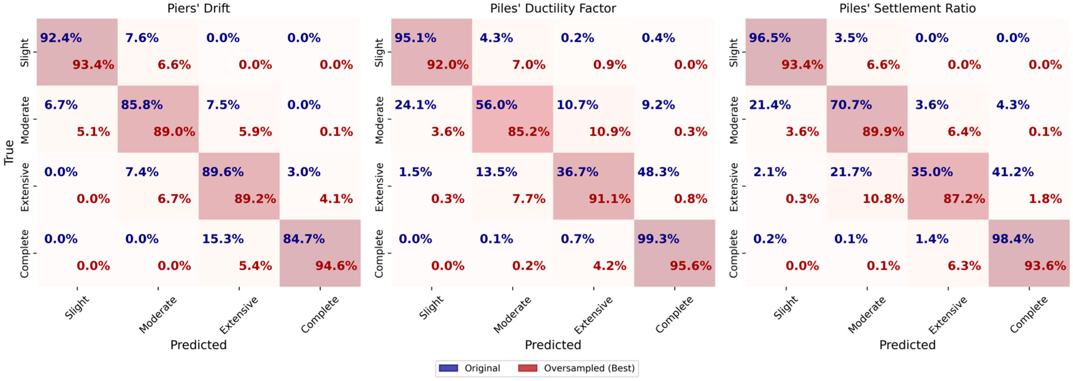
5.7. Random Forest (RF)

The Random Forest models are optimized using a grid search with hyperparameters including the number of trees, maximum tree depth, minimum samples required to split a node, and minimum samples per leaf. The model employed bootstrap sampling and used conservative depth limits to avoid overfitting while ensuring it could capture complex feature interactions.

For piers’ drift, the oversampled dataset yields the best performance (Figure 26), with an accuracy and F1-score of 0.91. The original dataset follows closely with both metrics at 0.89. The learning curves (Figure 27) show consistent improvements in cross-validation scores as more data are added, indicating robust generalization and the model’s ability to learn from additional training data. The oversampled dataset helps reduce overfitting and improves the model’s capacity to differentiate between damage levels. In contrast, the undersampled dataset shows reduced performance due to the limited number of training samples, which restricts the model’s ability to generalize effectively.

For HP DF, both the original and oversampled datasets result in accuracy and F1-score of 0.91, while the undersampled dataset drops to 0.79. Learning curves indicate signs of overfitting, especially for the oversampled dataset, though this effect diminishes as more samples are introduced. For HP SR, the model achieves an accuracy and F1-score of 0.88 on both the oversampled and original datasets, and 0.80 on the undersampled dataset. The learning curves indicate robust generalization for the oversampled dataset, while reduced generalization is observed for the undersampled dataset. Similarly to HP DF, oversampling for HP SR amplifies overfitting, highlighting the limitations of oversampling for these particular targets. The oversampled dataset allows the model to better learn the features necessary for distinguishing between different damage states, which is reflected in the improved performance. The undersampled dataset, however, results in a noticeable performance drop, suggesting that the model’s ability to generalize across varying damage levels is hindered by the lack of sufficient training data.

The Random Forest models demonstrate strong performance across all targets. For piers’ drift, the oversampled dataset reduces overfitting and improves generalization, while for HP DF and HP SR, oversampling amplifies overfitting. The oversampled datasets improves class distinction, but the undersampled datasets highlight the challenges of capturing finer distinctions between damage states due to limited sample sizes and reduced model generalization.

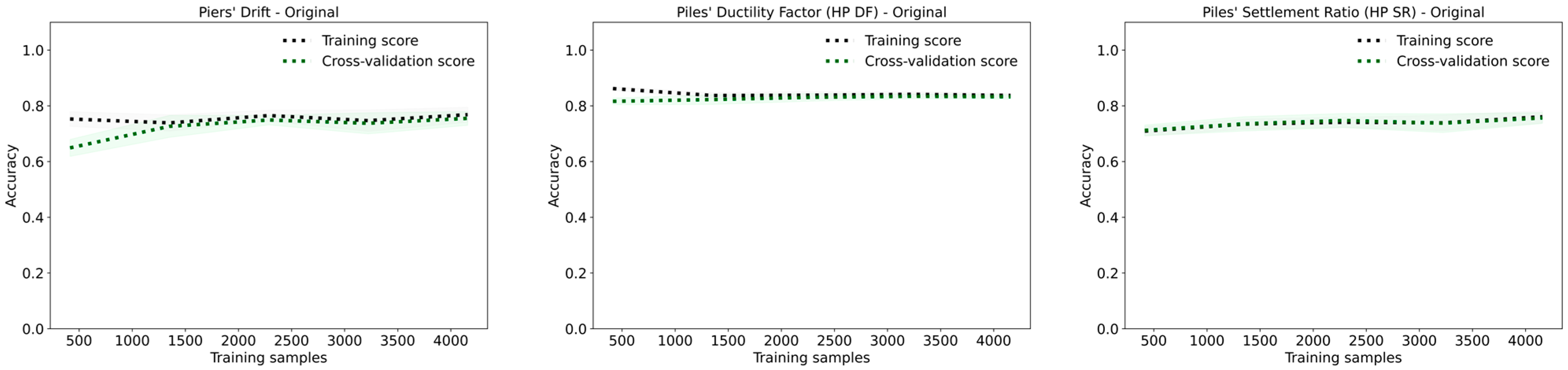
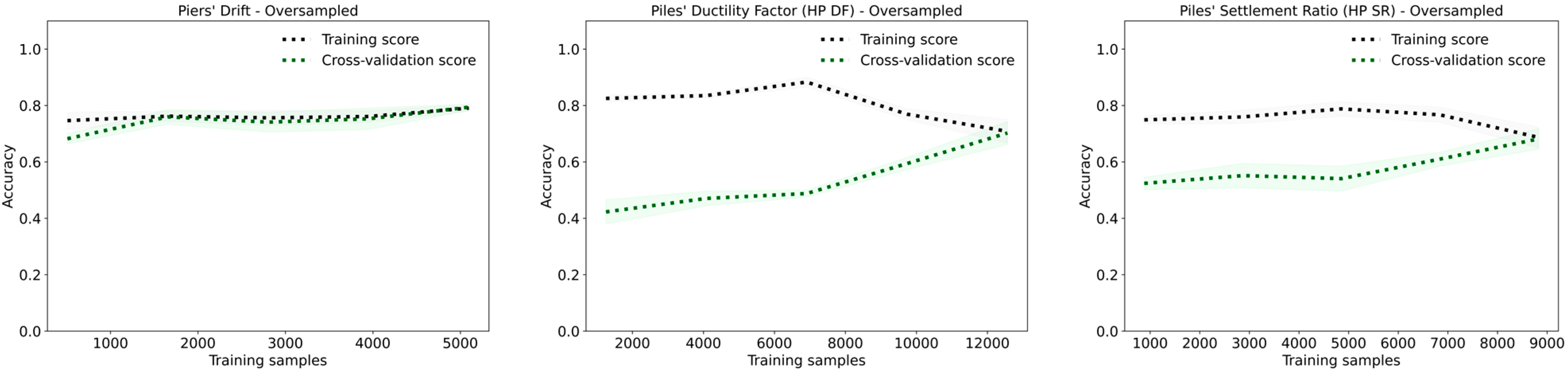
5.8. Artificial Neural Network (ANN)

The Artificial Neural Network (ANN) used in this study consisted of an input layer, two hidden layers, and an output layer. The network utilized ReLU activation functions for the hidden layers and a softmax activation function for the output layer. The optimization of hyperparameters is performed using a grid search, considering parameters such as the number of neurons in the hidden layers, learning rate, batch size, epochs, and optimizer type (e.g., Adam, SGD). The best parameters for each target are selected based on the highest stratified cross-validation score. Figure 28 displays the obtained confusion matrix and Figure 29 presents the learning curves for each target and dataset configuration. These plots illustrate the training and cross-validation accuracy as a function of the number of training samples. The learning curves provide insight into the model’s performance, showing the relationship between training size and model accuracy.

For the piers’ drift target, the original dataset achieves an accuracy and F1-score of 0.75. The oversampled dataset shows a slight improvement, reaching an accuracy and F1-score of 0.76. In the oversampled dataset, the accuracy of slight, moderate, extensive, and complete damage slightly decreases, while the accuracy of complete damage increases significantly. The undersampled dataset, however, performs worse with both accuracy and F1-score at 0.72.

The results for HP DF target indicate that the original dataset provides the highest accuracy of 0.84 and an F1-score of 0.80. The performance of the oversampled dataset is worse with an accuracy and F1-score of 0.74. The learning curves of the oversampled dataset further support this as the gap between curves is significant. The undersampled dataset gives an accuracy of 0.63 and an F1-score of 0.62. The learning curves of the undersampled dataset indicate that the model suffers from high variance, as the gap between the training and validation curves is obvious.

For HP SR, the original dataset achieves an accuracy of 0.76 and an F1-score of 0.72. The oversampled dataset gives an accuracy and F1-score of 0.68, while the undersampled dataset yields the lowest performance with an accuracy and F1-score of 0.59. The learning curves of the HP SR target show that as more samples are added, the validation score increases and eventually meets the training score. The training score shows a slight increase in accuracy up to 6000 samples, after which it underfits to meet the validation curve.

Overall, the results indicate that oversampling generally improves the classification performance compared to undersampling, particularly by enhancing the accuracy for certain damage levels, such as complete damage in the piers’ drift target. However, the original dataset often yields the best overall outcomes in terms of accuracy and F1-score, with minimal variance between training and validation performance, as seen in the learning curves. The undersampled dataset typically leads to lower accuracy and high variance, indicating the model’s inability to generalize well under limited data conditions.

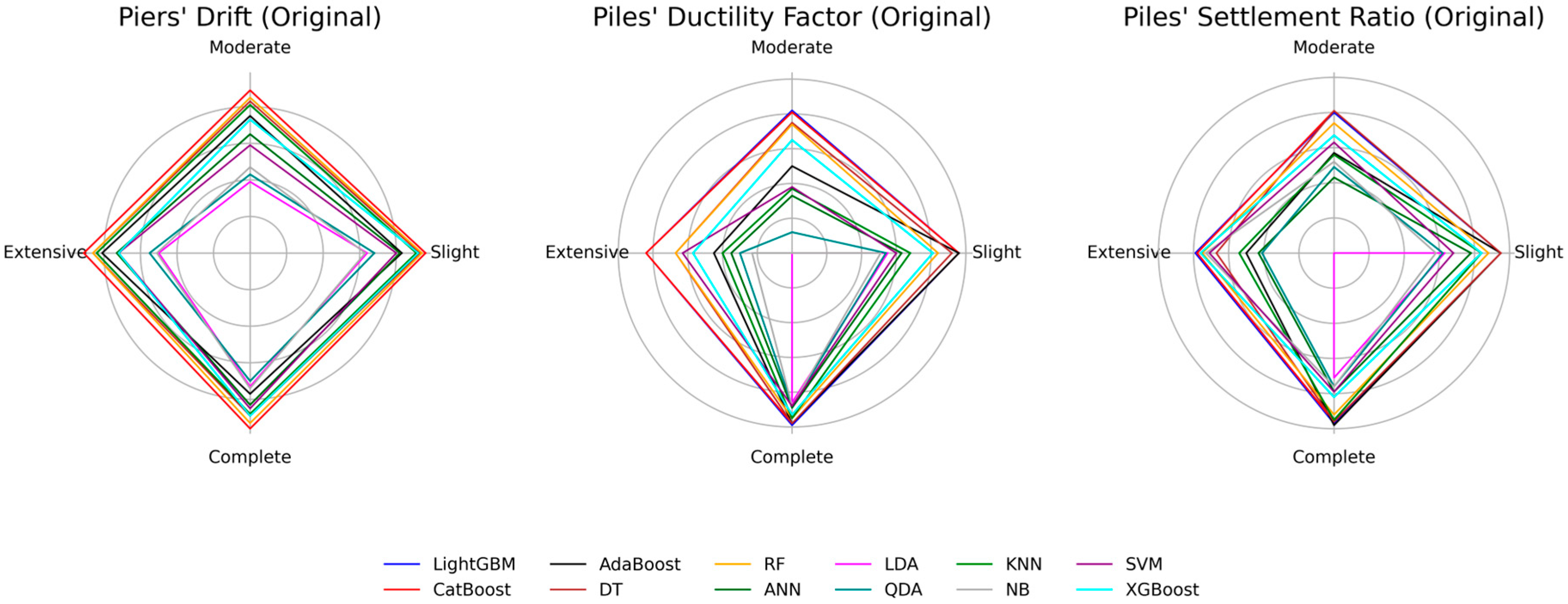
5.9. Comparison of Model Performances

Figure 30 illustrates radar charts for the original dataset that compare the classification performance of several machine learning algorithms for three bridge response metrics—piers’ drift, piles’ ductility factor (HP DF), and piles’ settlement ratio (HP SR)—across four damage states (slight, moderate, extensive, complete).

For piers’ drift with original dataset, CatBoost and LightGBM achieve the highest and nearly identical F1-scores, followed by RF, DT, and ANN. RF classifies the moderate class slightly better than DT and ANN, whereas LDA, QDA, and NB perform poorly, particularly for the moderate and extensive classes where sample sizes are limited.

For the HP DF target with the original dataset, LightGBM marginally outperforms CatBoost in the moderate damage class, while their results in other states remain comparable. In other classes, their performance is very similar. They are followed by RF and DT, with RF performing better in the extensive class and DT performing better in the slight class. AdaBoost performs well in classifying slight and complete damage classes, but its performance declines in other classes. The worst performing method in the HP DF target with the original dataset is LDA, as it failed to classify the extensive damage class. A similar pattern appears for HP SR: LightGBM and CatBoost lead, AdaBoost and ANN show moderate effectiveness in the Slight and Complete states, and LDA and QDA again have the weakest results.

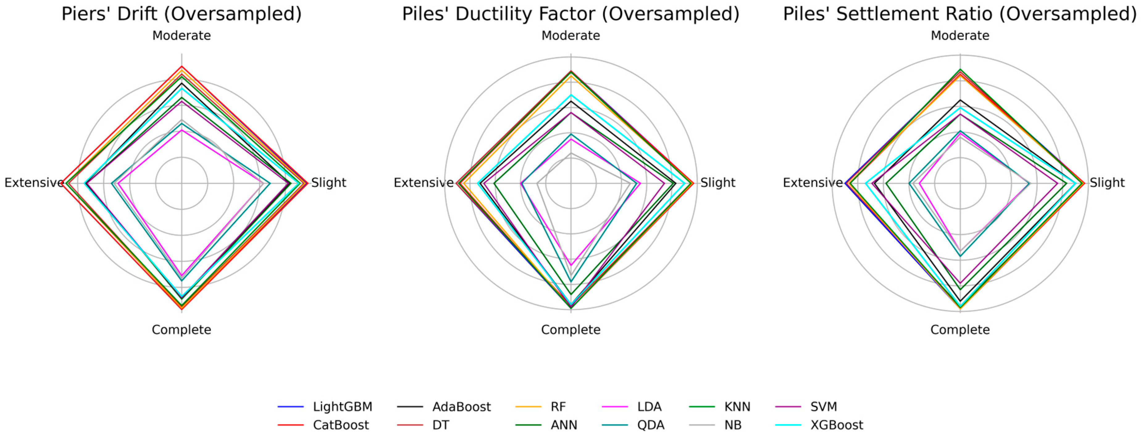
The oversampled dataset results across different targets shown in Figure 31 indicate a noticeable improvement only for the piers’ drift models, again led by LightGBM and CatBoost. Oversampling offers limited benefit for HP DF and HP SR and based on the learning curves, even promotes overfitting. This observation reflects the underlying imbalance in the original data, where HP DF and HP SR contain a large majority of complete class samples, whereas the piers’ drift target classes are more evenly distributed.

Figure 32 compares the performance of different algorithms using the undersampled dataset. The undersampled dataset generated employing the random undersampling method proved unsuitable, as it leads to reduced performance across all algorithms and targets compared to the original and oversampled datasets. This suggests the need for a more sophisticated undersampling method that can capture the nonlinearity between the target and features to effectively eliminate non-beneficial entries. Therefore, random undersampling is not recommended for such cases.

CatBoost and LightGBM remain less sensitive to oversampling because the gradient-boosting framework already applies internal row sampling and adaptive weighting during training. Duplicated minority-class samples, therefore, do not dominate the learning process, and each boosting iteration focuses on the most challenging observations. Their tree-based structure also captures nonlinear and interaction effects that are common in seismic response data without extensive feature scaling. In contrast, SVM relies on support vectors near the decision boundary, so duplicated minority samples can shift that boundary unrealistically, and ANN requires larger and truly independent datasets for generalization; synthetic duplicates can, therefore, encourage memorization rather than learning. Traditional linear classifiers such as LDA and QDA assume normally distributed classes and covariance structures that do not match the complex distributions encountered here, leading to consistently lower scores.

To sum up, LightGBM and CatBoost consistently deliver the highest and most stable F1-scores across the three targets and across different class-balancing strategies. Their robustness is attributed to efficient gradient boosting, built-in sampling, and the ability to model complex relationships in imbalanced seismic datasets with minimal parameter tuning, making them suitable baseline options for rapid damage classification in post-earthquake operations [48,49].

6. Conclusions

This study systematically evaluated the effectiveness of various machine learning algorithms in classifying damage states related to piers’ drift, piles’ ductility factor, and piles’ settlement ratio. The analysis provided valuable insights into the strengths and limitations of each algorithm, as well as the impact of data balancing techniques on classification performance. The following conclusions are drawn from the current study:

• Among all models, LightGBM and CatBoost consistently achieved the highest F1-scores across the three targets. Their robustness stems from advanced gradient boosting strategies, which internally manage class imbalance and feature interactions. Both models required minimal preprocessing and showed resilience to overfitting.
• Random Forest and Decision Tree classifiers performed well in distinguishing specific damage states. Random Forest was more effective in moderate and extensive classes, while Decision Trees achieved better classification in the slight damage class. These tree-based models offer transparent decision paths, which may be advantageous in practical engineering applications.
• AdaBoost and Artificial Neural Networks (ANN) performed adequately in majority classes but showed inconsistent results for underrepresented classes. ANN, in particular, was sensitive to the presence of synthetic samples in oversampled datasets, suggesting a need for larger, high-quality datasets to fully utilize its learning capacity.
• Linear and Quadratic Discriminant Analysis as well as Naïve Bayes exhibited the lowest performance. Their restrictive assumptions regarding data distribution and feature independence did not align with the complexity and nonlinearity inherent in seismic response data.
• Oversampling using SMOTE improved classification for the piers’ drift target, especially with LightGBM and CatBoost. However, it provided limited or even disadvantageous effects for HP DF and HP SR targets, where class imbalance was more severe. Oversampling in those cases often introduced redundant patterns, which increased overfitting risk in models like ANN and SVM.
• Random undersampling resulted in substantial performance degradation across all algorithms. It eliminated valuable samples that were essential for learning complex decision boundaries. Future studies should explore more informed sampling strategies, such as Tomek links or edited nearest neighbor, that reduce imbalance without discarding critical data.
• While the machine learning work proposed in this study shows promise for rapid seismic damage classification, several limitations must be acknowledged. The dataset originates from numerical simulations based on idealized OpenSees models, whose assumptions (e.g., material behavior, boundary conditions, interaction mechanisms) could affect model generalizability. The effects of these simplifications on the training data remain an open question.
• Moreover, the use of synthetic oversampling techniques introduces risks of overfitting, particularly when the original dataset is highly imbalanced. Although SMOTE helped improve minority class predictions in some cases, its synthetic samples do not necessarily reflect realistic structural responses and may compromise generalization.
• The scalability of the proposed models to real bridge inventories remains uncertain, as the training data were derived from simulations of a single bridge typology. To improve real-world applicability, future work should integrate observational data or inspection records from a wider range of bridge types, site conditions, and structural configurations.

In summary, gradient boosting models such as LightGBM and CatBoost emerged as reliable and high-performing tools for seismic damage classification. However, the application of machine learning in this domain must carefully consider data origin, balancing techniques, and representativeness of structural scenarios. Addressing these limitations will be crucial for translating the developed models into operational tools for post-earthquake response and infrastructure resilience planning.