Hybrid Machine Learning Model for Predicting the Fatigue Life of Plain Concrete Under Cyclic Compression

Abstract

Accurately predicting the fatigue life of concrete is crucial for ensuring the safety and durability of structural elements subjected to cyclic loading. Traditional empirical models often struggle to capture the complex interactions between mechanical properties and loading conditions, particularly the influence of frequency. This study introduces a hybrid machine learning model based on the stacking ensemble strategy, integrating Support Vector Regression (SVR), Random Forest (RF), and Artificial Neural Networks (ANNs) to enhance prediction accuracy. A dataset of 891 experimental results from the literature was utilized, incorporating four key input variables: compressive strength, stress ratio, maximum stress-to-strength ratio, and loading frequency. The hybrid model demonstrated superior performance (R² = 0.965, RMSE = 0.19), outperforming individual models and established predictive equations. SHAP analysis validated the model’s interpretability and emphasized the necessity of accounting for loading frequency. This study contributes a robust and generalizable tool for fatigue life prediction within the defined input domain, offering valuable insights for engineering design and structural assessment.

1. Introduction

Concrete structures experience cyclic loads derived from several sources, including static and dynamic loads, such as dead and live loads in building settings and traffic-induced loads in civil engineering applications. Furthermore, these structures are vulnerable to climatic factors, such as temperature and humidity variations.

Concrete’s mechanical strength decreases when exposed to repetitive cyclic loading. This phenomenon, known as fatigue, is widely recognized in the field of structural and material engineering and extensively documented in the literature [1,2,3,4,5].

Fatigue is a phenomenon that causes localized, permanent, and progressive damage when the composite is subjected to cyclic loads. The degradation of concrete by fatigue is associated with its deterioration when subjected to repeated loading and unloading, causing the initiation and propagation of cracks in the material [6].

Callister and Rethwisch [7] indicated that the cracks caused in concrete due to fatigue are fragile, with little or no plastic strain associated with the damage’s evolution. From the first micro-crack until the failure, concrete damage due to fatigue can be characterized in three stages, based on the strain levels: (i) crack initiation, which occurs when the micro-cracks appear due to high stress concentrations at points of discontinuity in the crystalline structure or regions with pre-existing discontinuities; (ii) crack propagation, associated with the accumulation of energy at the ends of existing cracks; and (iii) material failure, which occurs abruptly, due to the quasi-brittle nature of the composite.

To estimate concrete’s fatigue life (i.e., the number of cycles to failure, N), it is necessary to understand the material’s mechanical behavior under cyclic loads. Materials’ fatigue life is usually defined by experimental test results, where the specific stress or strain is plotted as a function of the logarithm of the cycle number, characterizing the S-N and ε-N curves, respectively, known as Wöhler curves.

Several models exist in the literature for predicting the fatigue life of concrete. Equations (1)–(6) present some of them, where $\sigma$_max is the maximum stress applied, N is the number of cycles to failure, and d and e are material parameters obtained by data fitting. R is the minimum-to-maximum stress ratio, f_est is the compressive or tensile strength, ${\dot{\epsilon }}_{sec}$ is the secondary creep rate, ${\sigma }_{b,d,max}$ is the design value of the maximum stress, $f_{b,v}$ is the fatigue reference strength, Υ is a parameter defined in the fib Model Code [8], $S_{c,max}$ is the maximum stress-to-strength ratio, and S_c,min is the minimum stress-to-compressive-strength ratio.

$${\displaystyle \frac{{\sigma }_{max}}{f_{est}}}=d+e log\left(N\right)$$

(1)

$$log\left(N\right)=13.275-11.39\left({\displaystyle \frac{{\sigma }_{max}}{f_{ck}}}\right)$$

(2)

$${\displaystyle \frac{{\sigma }_{max}}{f_{est}}}=1-0.0685\left(1-R\right)log\left(N\right)$$

(3)

$$log\left(N\right)=-2.66-0.94log\left({\dot{\epsilon }}_{sec}\right)$$

(4)

$$log\left(N\right)={\displaystyle \frac{10}{\sqrt{1-R}}}\left(1-{\displaystyle \frac{{\sigma }_{b,d,max}}{f_{b,v}}}\right)for{\displaystyle \frac{{\sigma }_{b,d,max}}{f_{b,v}}}>0.25$$

(5)

$$\begin{gathered} LogN=\left\{\begin{array}{c}log{N}_{1}iflog{N}_1\le 8\\ log{N}_{2}iflog{N}_1>8\end{array}\right. \\ log{N}_1={\displaystyle \frac{8}{{\rm Y}-1}}\left(S_{c,max}-1\right) \\ log{N}_2=8+{\displaystyle \frac{8ln\left(10\right)}{{\rm Y}-1}}\left({\rm Y}-S_{c,min}\right)log\left({\displaystyle \frac{S_{c,max}-S_{c,min}}{{\rm Y}-S_{c,min}}}\right) \end{gathered}$$

(6)

Equation (1) represents a traditional linear correlation between the highest level of stress and the logarithm of the fatigue life, known as the Wöhler curve. Equations (2)–(4), proposed by Raithby and Galloway [9], Sparks [10], and Tepfers and Kutti [11], respectively, are derived from the Wöhler curve and were defined with data from the experimental results.

According to the Dutch National Code NEN 6723:2009 [12], the fatigue life can be estimated by Equation (5). The formulation specifies that if the ratio of the maximum compressive strength to the fatigue reference strength does not surpass 0.25, the concrete’s fatigue life could be considered infinite. According to the fib Model Code [8], Equation (6) forecasts the fatigue life of concrete under compression cycles. The formulation was generated based on experimental results from a fatigue test performed on ultra-high-strength concrete. Equation (6) was also validated for estimating the fatigue life of high- and conventional-strength concrete.

Most earlier investigations have examined these equations, and the results have demonstrated that formulations based on the S-N curve cannot generalize performance and, in most cases, are inadequate to characterize the fatigue behavior of plain concrete [13,14,15]. Lee and Barr [16] presented multiple reasons why models based on the Wöhler curve are impractical. The primary challenge arises from the need to calibrate the model parameters using experimental data. Thus, numerous models developed based on the Wöhler curve are limited by certain boundary conditions, thereby restricting their applicability. Furthermore, there is the challenge of accurately adjusting the input parameters of the models due to the significant deviations in fatigue life results obtained under tests with identical boundary conditions [14,17,18].

Ortega et al. [14] described how the significant deviation observed in the fatigue life results can be attributed to the fact that fatigue strength is highly influenced by multiple variables associated with the boundary conditions of the experimental tests and the material’s heterogeneity. These parameters, such as concrete molding and cure conditions, specimen alignment in the test machine, specimen shape, precise imposition of maximum and minimum stress values, loading frequency, and positioning of strain gauges, are difficult to control.

Additionally, one of the most significant issues in characterizing concrete’s fatigue life using models based on S-N or ε-N curves is the requirement to test numerous samples for each stress level, as the results have a high degree of deviation. An alternative approach to addressing this issue is the application of probability and reliability theories to assess the confidence level associated with the sample size used in analyses [19,20,21,22,23]. Additionally, machine learning techniques [15,24,25] offer the advantage of incorporating multiple parameters related to the phenomenon, capturing the intricate and nonlinear relationships between them, and ultimately mitigating the high variability in results.

The first publication about machine learning in civil engineering was by Adeli and Yeh [26]. They presented a perceptron ANN to design steel beams. After that, some research using machine learning in civil engineering was developed, focusing on pattern recognition, data mapping, and classification.

Machine learning has also been widely applied in geotechnical engineering. Williams and Gucunski [27] used backpropagation neural networks to estimate average soil thickness and elastic properties, while Goh [28] showed that ANNs could correlate soil parameters obtained from laboratory tests. Subsequent studies further confirmed that machine learning techniques are effective in defining soil constitutive models and predicting the mechanical behavior of geomaterials [29,30,31,32,33].

Nevertheless, since the pioneering work of Adeli and Yeh [26], the application of Artificial Neural Networks has predominantly focused on structures and materials within civil engineering. In structural engineering, ML has been employed for the design and analysis of structural components [34,35,36,37,38,39,40,41] and analyses involving structural dynamics, impacts, and earthquake effects [42,43,44,45]. ANNs have also proven valuable for damage assessment and risk management [46,47,48,49].

The use of machine learning techniques to predict concrete’s mechanical properties has recently gained popularity, including the use of Support Vector Machines (SVMs) [50,51,52], decision trees (DTs), Artificial Neural Networks (ANNs) [53,54,55,56], Random Forests (RFs) [57,58,59,60], and ensemble algorithms [61,62,63,64,65].

Abambres and Lantsoght [53] mapped the strength reduction of concrete when subjected to cyclic compression by Artificial Neural Networks. The authors utilized a dataset with 203 results extracted from the literature. An optimal neural network architecture was identified by systematically exploring and optimizing 14 neural network features. The model demonstrated its efficacy, achieving a maximum relative error of 5.1% and a mean relative error of 1.2% when predicting the reduction in strength due to the fatigue phenomenon. Furthermore, the proposed model surpassed existing code expressions, yielding a mean tested-to-predicted value of 1.00, with a coefficient of variation of 1.7%.

Zheng et al. [56] utilized Artificial Neural Networks to predict fatigue failure mechanisms in cementitious materials by analyzing a dataset of 314 cases from the literature. The ANN model integrated seven cement variables and seven test boundary parameters as input parameters. The authors conducted a thorough feature selection analysis, exploring 150 combinations, and refined the ANN through backpropagation tuning. The model achieved an impressive accuracy of up to 90.78%, demonstrating its efficiency in mapping the fatigue failure mechanisms.

Using Artificial Neural Networks, Support Vector Machines, and Random Forests, Zhang et al. [24] generated models to predict the residual strength of concrete under cyclic loading, in which a strength degradation model was proposed to evaluate the residual strength. The authors utilized over 1000 experimental data points gathered from various sources in the literature. The results indicated that the Random Forest algorithm is the most effective strategy for mapping fatigue life, as it has superior performance metrics. Specifically, it achieved a mean squared error of 0.44 and a determination coefficient (R²) of 0.72. The results of this study demonstrate the significant challenges in establishing a correlation between input parameters and fatigue life when dealing with a large dataset. The metric performances highlight the high complexity involved in this process.

Using the same dataset as Zhang et al. [24], Son and Yang [15] developed models to forecast concrete’s fatigue life using Random Forests, Artificial Neural Networks, gradient boosting, and AdaBoost techniques. Due to the high deviation in the experimental results of fatigue life, the modeling was performed considering three strategies for structuring the database and evaluating its influences on the learning process: (i) all of the data were used to map the fatigue life (1298 data), (ii) the dataset was reduced by excluding outliers (1252 data), and (iii) the model was developed with average fatigue life excluding outliers (resulting in 310 data). To evaluate the model’s generalization, 10% of the data were used for the test set. With this procedure, the model’s prediction performance was significantly enhanced, with the coefficient of determination (R²) increasing to 0.635 when trained on the entire dataset using the ANN, and to 0.730 for the average data, excluding outliers.

In recent years, ensemble learning techniques have gained significant attention for improving the predictive performance of machine learning models in civil engineering applications, particularly in mapping the mechanical properties of concrete [62,64,65,66,67,68]. Ensemble methods combine the predictions of multiple base models to enhance accuracy, robustness, and generalization. Among the most common ensemble strategies are bagging, boosting, and stacking. Bagging, or bootstrap aggregation, trains several models independently on different random subsets of the training data and averages their outputs, effectively reducing variance and mitigating overfitting; Random Forests are a classical example of this approach [60]. Boosting, in contrast, sequentially trains models, with each new model focusing on correcting the errors of its predecessor, which tends to reduce bias and achieve higher accuracy, although it may be more sensitive to noise and overfitting. Models based on XGBoost and LightGBM have shown remarkable results in predicting concrete’s strength [69,70,71]. Stacking, however, builds a hybrid model by training a meta-learner to optimally combine the outputs of several base learners, offering a flexible framework that is capable of capturing complex data patterns across different types of models [68,72,73,74]. Unlike bagging and boosting, which usually use homogeneous base models, stacking often employs heterogeneous models, such as combining neural networks, decision trees, and Support Vector Machines, resulting in more versatile and powerful predictive tools.

Considering the recent developments in concrete fatigue life prediction models based on machine learning techniques, and given the current application of ensemble learning techniques to enhance models’ accuracy, this study explores the use of Artificial Neural Networks (ANNs), Random Forests (RFs), and Support Vector Regression (SVR) coupled through the stacking fusion strategy to generate a new approach to forecasting concrete’s fatigue life. The stack fusion strategy combines multiple base machine learning models’ strengths while mitigating their weaknesses [66]. The models were proposed based on a dataset comprising 891 experimental results of concrete tested with constant amplitude and loading frequencies ranging from 1 to 10 Hz (high frequency). The models were built to attend to the different demands of the design or construction phases, considering four input parameters that are easily obtained and processed: the concrete’s compressive strength (FC), the maximum stress applied–concrete compressive strength ratio (SMAX), the minimum-to-maximum stress ratio (R), and the load frequency (FHZ).

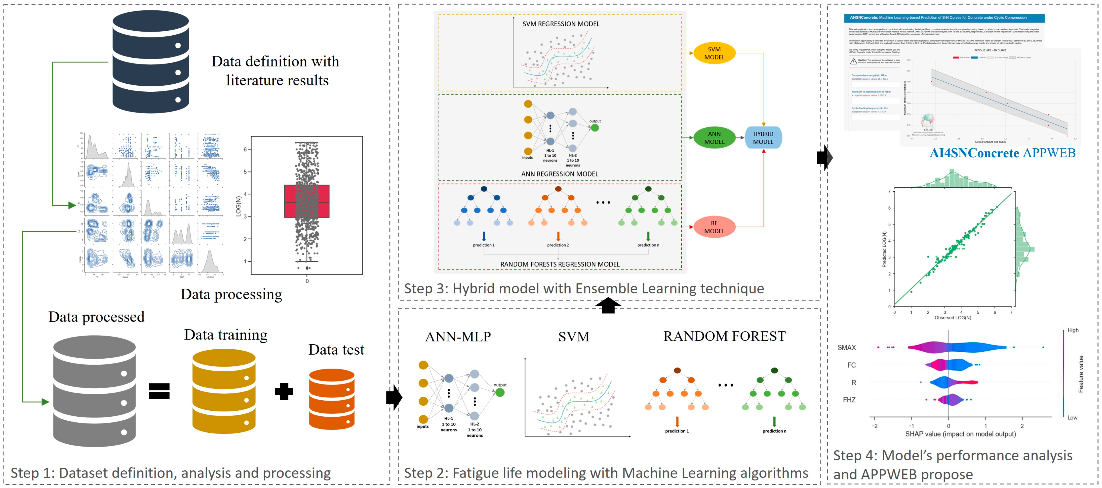
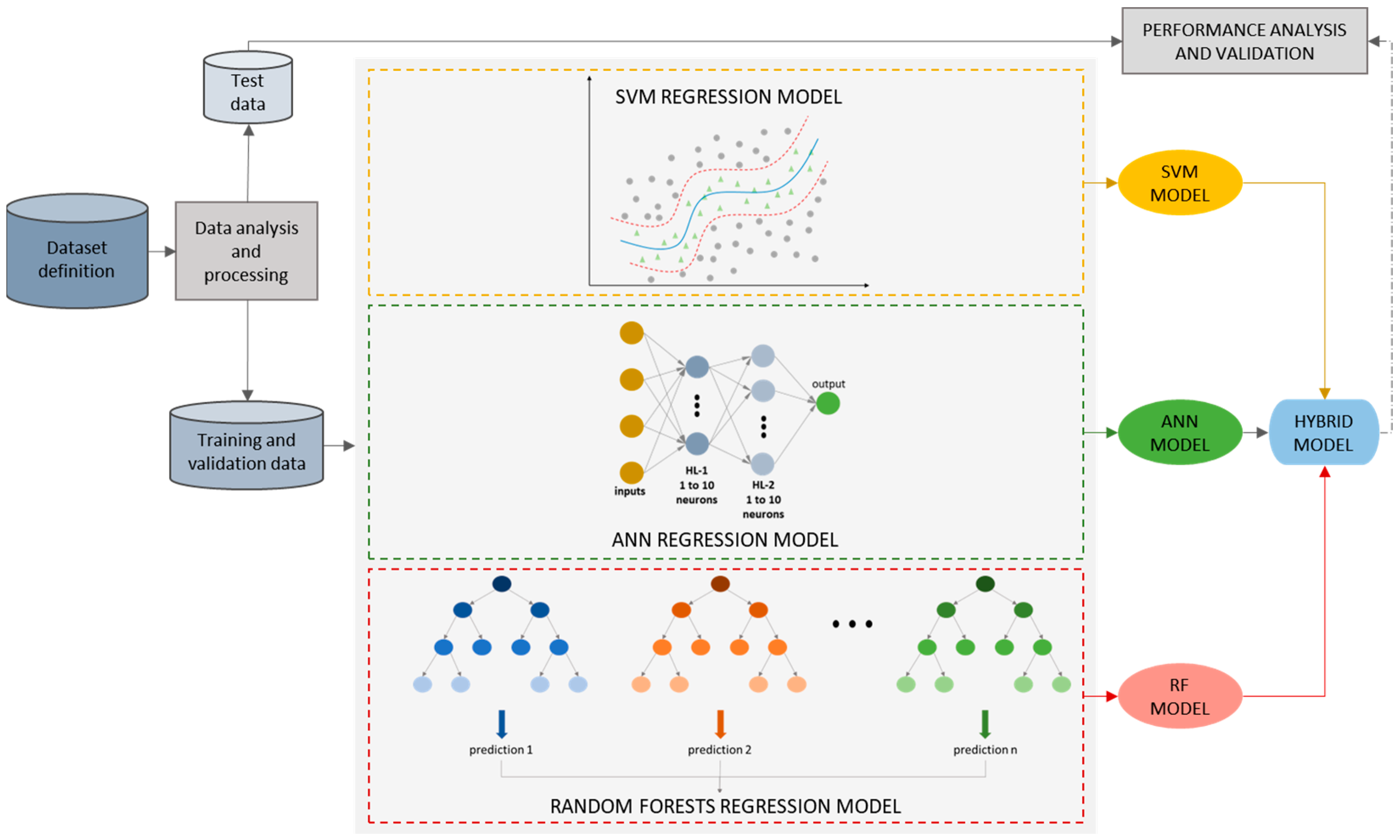
2. Data Processing and Modeling

Following the procedure depicted in Figure 1, the ensemble learning technique with the stacking fusion strategy was applied to create a hybrid machine learning model for forecasting the fatigue life of plain concrete.

The methodology used to design the hybrid model considers coupling the fatigue life values predicted by the SVM, ANN, and RF base models. The dataset definition and processing, development of the base machine learning models, creation of the hybrid model, and analysis of the model’s performance are described below. The code was built in Python (version 3.11.4), and the machine learning models were trained with the Scikit-learn package (version 1.5.2) [75].

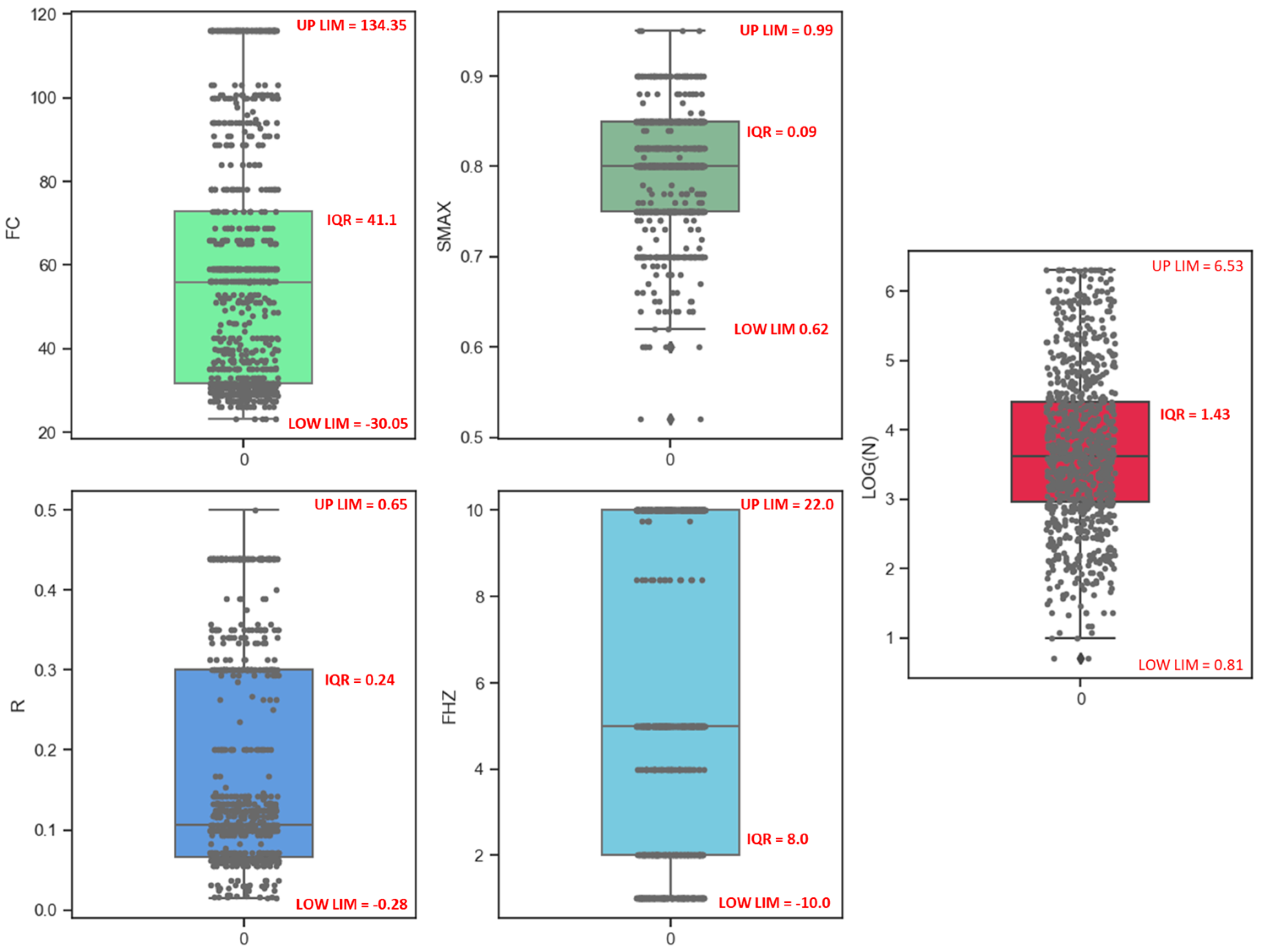
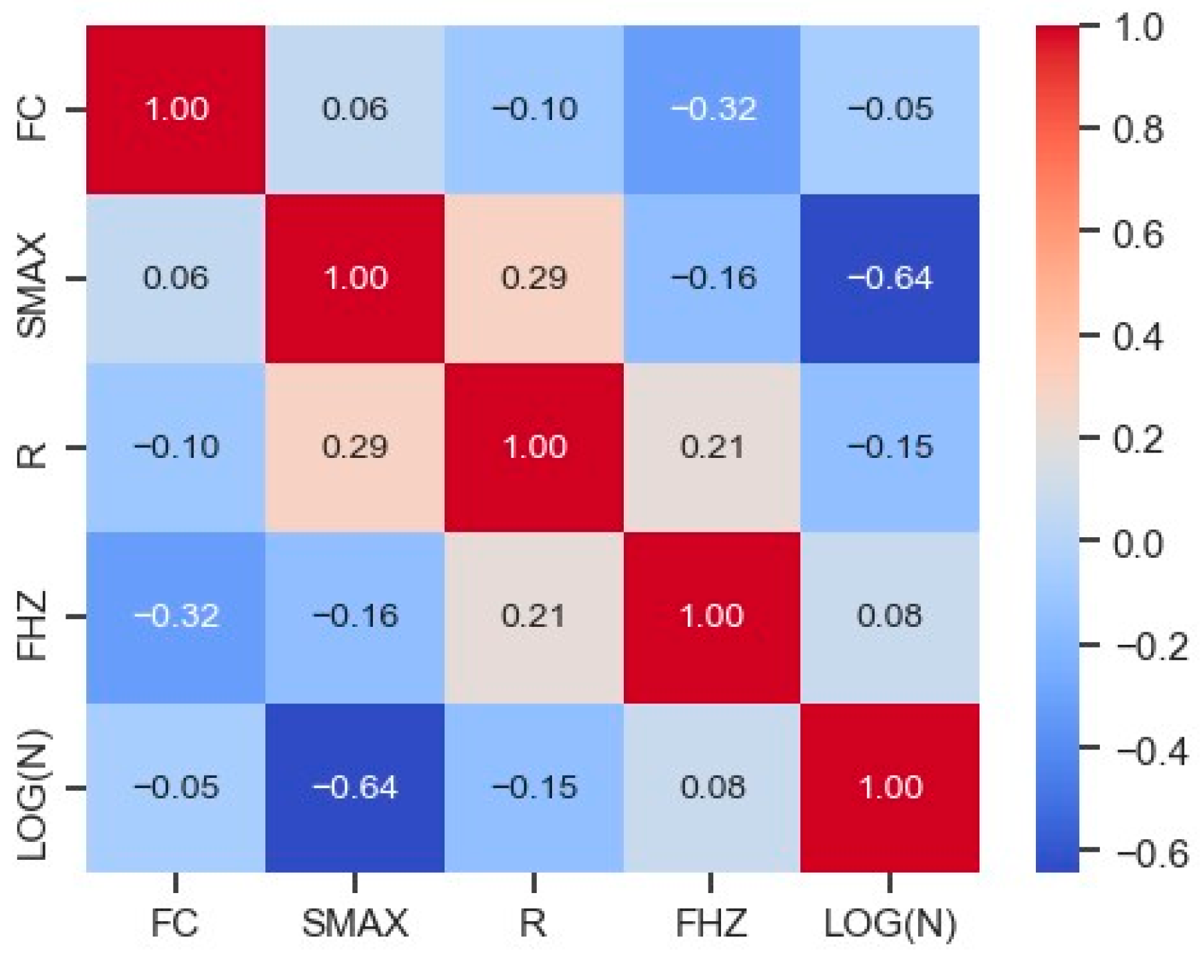
2.1. Dataset Definition, Analysis, and Processing

The definition of a database containing reliable and representative data is the first and foremost step for developing a model. Thus, a database was set up considering experimental campaigns published in the last three decades [3,11,14,15,19,24,76,77,78,79,80,81,82,83,84,85,86,87,88]. In total, 891 data points referring to concrete with a compressive strength between 20 and 120 MPa were collected, whose fatigue tests were conducted at loading frequencies ranging from 1 to 10 Hz, with maximum stress levels varying between 50% and 95% of the compressive strength. To attend to the different demands of the reinforced concrete’s design or construction phases, in the dataset collection, four input parameters were defined as possible input parameters: the concrete’s compressive static strength (FC), the maximum stress applied–compressive strength ratio (Smax), the minimum-to-maximum stress ratio (R), and the load frequency (FHZ). The output N, representing the number of cycles to failure, was converted to LOG(N) to reduce the domain of the variable.

Table 1. Data on statistical parameters.

Feature	Minimum	Maximum	Standard Deviation	Mean	Q1 (25%)	Q2 (50%)	Q3 (75%)
FC (MPa)	23.10	116.00	29.02	57.47	31.60	55.80	72.70
SMAX	0.52	0.95	0.06	0.79	0.75	0.80	0.84
R	0.01	0.50	0.13	0.17	0.06	0.10	0.30
FHZ (Hz)	1.00	10.00	3.65	5.84	2.00	5.00	10.00
N (cycles)	5.00	2.00E6	3.31E5	1.09E5	9.18E2	4.20E3	2.50E4
LOG(N)	0.69	6.30	1.14	3.72	2.96	3.62	4.39

presents the statistical features of the original data, providing the information needed to describe the data distribution pattern and identify outliers.

The interquartile range (IQR) outlier detection method was applied to the original dataset to enhance the training performance of the machine learning techniques. Outliers are observations that deviate from the norm. The IQR is calculated by the difference between the third (Q3) and first (Q1) quartiles, as indicated in Equation (7). After computing the IQR, it is advisable to remove data from the database with attributes that have values either above the upper limit (UPLIM) or below the lower limit (LOWLIM), as calculated by Equations (8) and (9), respectively.

$$IQR=Q3-Q1$$

(7)

$$UPLIM=Q3+1.5\left(IQR\right)$$

(8)

$$LOWLIM=Q1-1.5\left(IQR\right)$$

(9)

Figure 2 depicts a data distribution boxplot for the input features and LOG(N), as the values of IQR, UPLIM, and LOWLIM. Data exceeding the upper and lower limits were removed, resulting in a reduced initial database of 870 samples. As can be observed in Figure 2, only the minimum values of Smax and LOG(N) were changed. The minimum value of Smax changed from 0.52 to 0.62, while the minimum of LOG(N) assumed a value of 1.0. Figure 3 shows the data distribution after removing the outliers, and Figure 4 shows the Pearson correlation matrix.

For the values presented in Figure 4, most of the input variables exhibit low-to-moderate linear correlations with each other, with the highest absolute value being −0.64 between SMAX and LOG(N). This suggests that multicollinearity is not a critical concern among the predictors, supporting their simultaneous use in the model. It is important to emphasize that low Pearson correlation coefficients do not necessarily imply that a variable is unimportant for the predictive model. Rather, such variables may contribute through nonlinear or interaction effects, which are effectively captured by machine learning algorithms. Therefore, even features with weak linear associations, such as FC and LOG(N) (r = −0.05), can still significantly improve the model’s performance.

After eliminating outliers from the original dataset, instances where input attributes were repeated but linked to different target values (LOG(N)) were analyzed. In these specific cases, the mean, Q1, Q3, mode, and median of LOG(N) were computed, generating five information for each case, and then the duplicate entries were removed. The input features were standardized, and the dataset was divided into two subsets: 80% for training and internal cross-validation, and 20% for testing. Stratified sampling was applied based on the LOG(N) target variable to ensure a balanced representation of the response variable across both subsets. Specifically, the continuous LOG(N) values were discretized into 15 bins, uniformly spaced between 0.9 and 6.5, to preserve the overall distribution profile in the stratification process. This strategy helped maintain the statistical consistency of the response variable across the training and testing sets, thereby improving the robustness of the model evaluation.

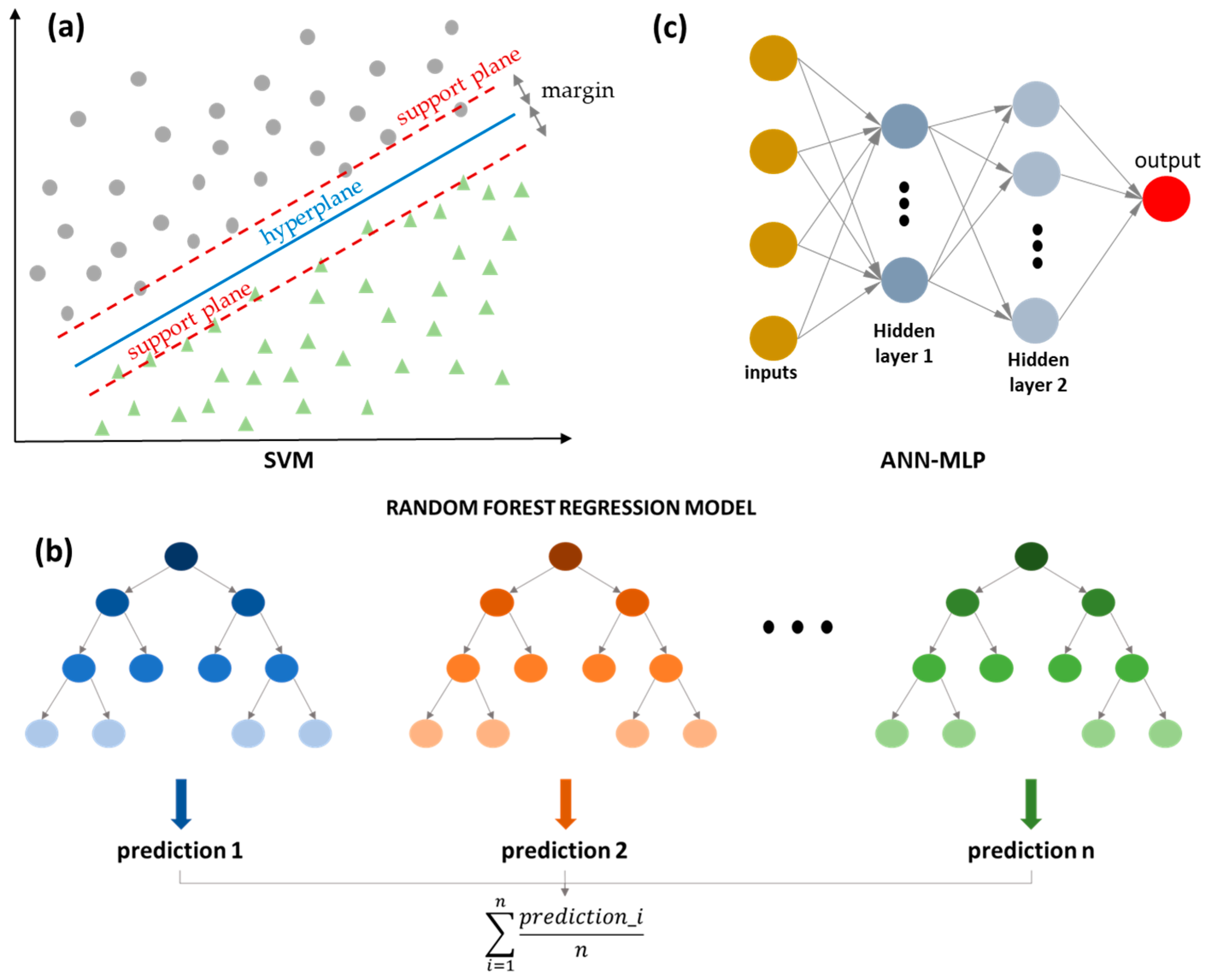
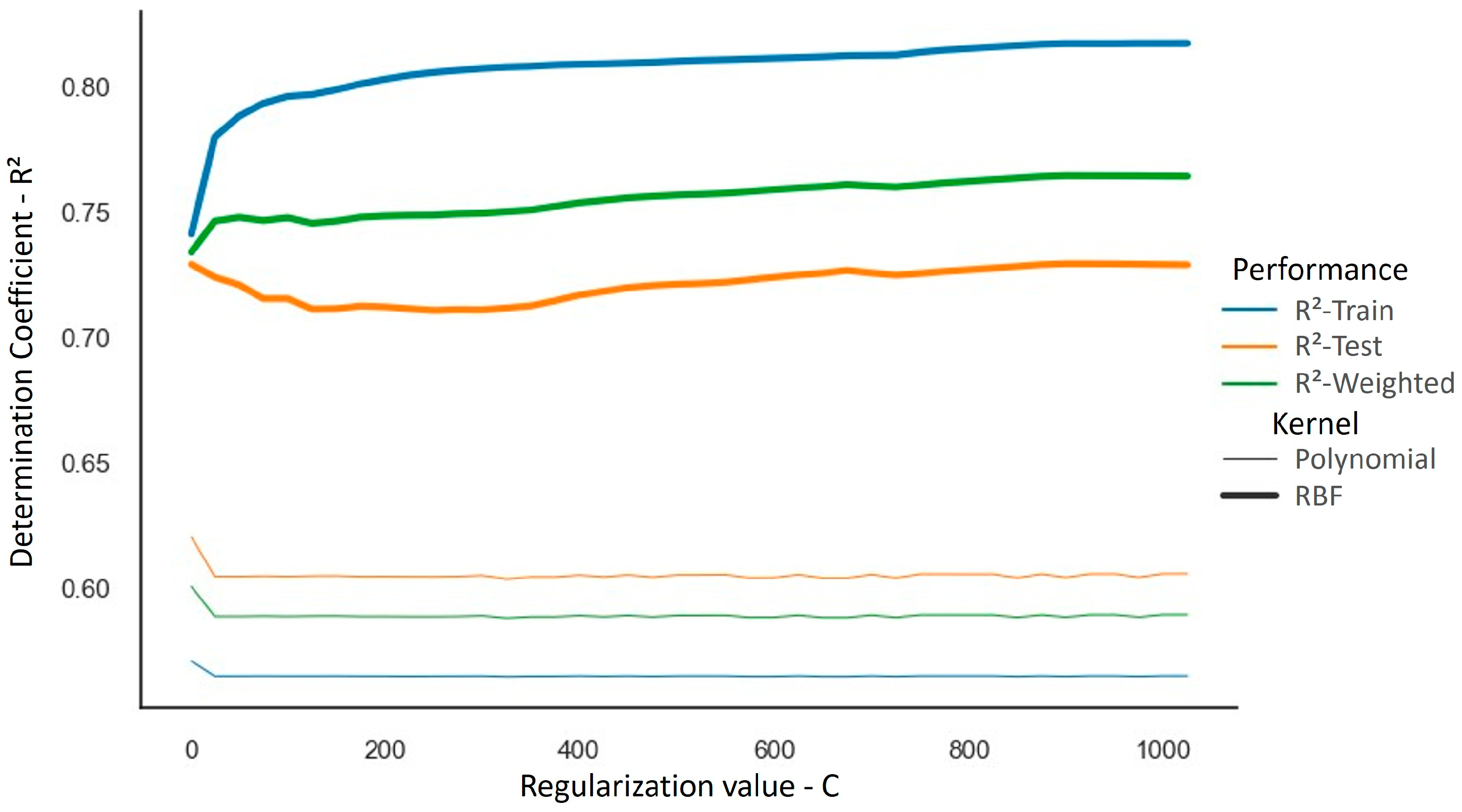
2.2. Machine Learning Algorithms

Support Vector Machine (SVM) is a supervised machine learning algorithm that is used for classification tasks and can be adapted for regression. SVM works by finding the hyperplane that best separates the data points into different classes or predicts the target variable in the topic studied by fitting a hyperplane to the data (Figure 5a). The key concept is to maximize the margin between the hyperplane and the closest data points from each class, referred to as support vectors. Maximizing the margin aims to achieve better generalization performance, making the model less sensitive to outliers.

In regression tasks, SVM aims to find a hyperplane that best fits the data points within a specified tolerance margin, minimizing the deviation of the predicted values from the actual values. SVM can handle linear and nonlinear relationships between the input features and the target variable using kernel functions, such as linear, polynomial, radial basis function (RBF), or sigmoid kernels. These kernels allow for the mapping of the input features into higher-dimensional spaces, where the data may become more separable or better approximated. A key parameter in the SVM formulation is the regularization parameter C, which controls the trade-off between the model’s complexity and the degree to which deviations larger than the margin are tolerated. A small C value encourages a smoother function that tolerates larger errors. In contrast, a large C penalizes deviations more heavily, potentially leading to overfitting if the model tries to fit the training data too closely.

A Random Forest (RF) is a versatile machine learning algorithm for classification and regression tasks. It belongs to the ensemble learning family and is known for its effectiveness in handling complex datasets. A Random Forest consists of a collection of decision trees, each trained on a random subset of the training data and using a random subset of the features (Figure 5b). During the training process, the algorithm constructs multiple decision trees independently, allowing them to work in parallel. This process introduces diversity into the model, as each tree learns different aspects of the data.

When making predictions, each tree in the forest independently predicts the target variable, and the final prediction is determined by aggregating the predictions of all trees. Then, in regression tasks, this aggregation is carried out by averaging the individual predictions of the trees. The randomness helps to mitigate overfitting, as each tree is trained on a different subset of the data and features. Additionally, RFs can handle high-dimensional datasets with many features, making them suitable for various applications.

An Artificial Neural Network (ANN) is a computational model inspired by the structure and functioning of the human brain’s neural networks. It is a versatile and powerful machine learning algorithm that is capable of learning complex patterns and relationships from data. Information flows through interconnected nodes organized into distinct layers: an input layer, one or more hidden layers (such as Multi-Layer Perceptron ANNs), and an output layer. Each node, also known as a neuron, receives input signals, processes them using an activation function, and passes the output to the next layer (Figure 5c).

During the training phase, the weights and biases of the connections between neurons are adjusted iteratively using optimization algorithms, such as gradient descent, to minimize the difference between the model’s predictions and the actual target values. This process is known as backpropagation. ANNs can be applied to various machine learning tasks, including classification, regression, and clustering. They are particularly well suited for tasks involving complex, nonlinear relationships between the input and output variables.

In this work, machine learning models based on Support Vector Machines (SVMs), Random Forests (RFs), and Artificial Neural Networks (ANNs) were developed to serve as base learners in the hybrid modeling framework. For the SVM models, a systematic search was conducted involving 2000 configurations generated by varying the kernel type (polynomial and radial basis function (RBF)) and the regularization parameter C, which ranged from 1 to 1000. Each model was evaluated under identical conditions to identify those providing the best trade-off between bias and variance. The epsilon-insensitive loss function was employed, and the remaining hyperparameters followed standard configurations, including automatic gamma scaling and the shrinking heuristic to improve computational efficiency.

Regarding the Random Forest models, 396 different configurations were trained and evaluated. The study considered four distinct split criteria—squared error, absolute error, Friedman MSE, and Poisson error—to assess the quality of the node divisions. Forests composed of varying numbers of decision trees (from 2 to 100) were analyzed. The final training strategy employed parameters such as absolute error as the split criterion, a maximum tree depth of 50, and using all features per split to enhance generalization while maintaining model interpretability.

For the ANN, 400 architectures were tested using a Multi-Layer Perceptron framework with two hidden layers. The number of neurons in each layer varied from 1 to 20, and the activation function was set as logistic. The networks were trained using the backpropagation algorithm with the Adam optimizer, employing an adaptive learning rate initialized at 0.4. Regularization was applied through an L2 penalty (α = 0.0001). Additional training settings included a momentum of 0.9, with training for up to 10⁶ iterations or until the convergence criteria were met. The weight initialization was set to 0.5, following the same strategy used in [89].

Hyperparameter tuning was conducted using a grid search strategy for all base models. Each configuration was evaluated through 10-fold cross-validation, applied to the same training dataset (80% of the full dataset), with stratified sampling based on the target variable to preserve the distribution of fatigue life (LOG(N)). This consistent evaluation framework ensured fair comparisons among the models and robust generalization performance, as described in the data preprocessing section.

2.3. Hybrid Model Development

The hybrid model was constructed using a stack fusion strategy, an ensemble learning technique that linearly combines the outputs of multiple base models to enhance predictive performance while reducing individual model weaknesses [66]. Specifically, the hybrid prediction of LOG(N) is obtained as a weighted linear combination of the outputs predicted by the best-performing SVM, RF, and ANN models. This combination is represented by Equation (10), and its structure is shown in Figure 6. Specifically, the predictions of each base model for the training and test set—$LOG{\left(N\right)}_{SVM}$, $LOG{\left(N\right)}_{RF}$, and $LOG{\left(N\right)}_{ANN}$—are used as explanatory variables in a multiple linear regression model, while the observed values of LOG(N) from the test set serve as the response variable.

The coefficients ${\beta }_{SVM}$, ${\beta }_{RF}$, and ${\beta }_{ANN}$, along with the intercept term $\epsilon$, are estimated using the Ordinary Least Squares (OLS) method. This procedure enables the hybrid model to learn the optimal weighting of each base model’s prediction, resulting in a final estimate that leverages the strengths of each individual model based on their actual performance on unseen data.

$$LOG\left(N\right)={\beta }_{SVM}LOG{\left(N\right)}_{SVM}+{\beta }_{RF}LOG{\left(N\right)}_{RF}+{\beta }_{ANN}LOG{\left(N\right)}_{ANN}+\epsilon$$

(10)

SVM’s strength is finding optimal hyperplanes to separate data points or predict continuous values. This is particularly useful for its robustness to outliers and ability to handle nonlinear relationships. Random Forests leverage multiple decision trees to mitigate overfitting and handle high-dimensional datasets, contributing to their robustness. With its capacity to learn complex patterns, the ANN complements the ensemble by effectively modeling nonlinear functions.

By combining these techniques, the hybrid ensemble model leverages the diverse perspectives and strengths of each method. This enables the model to capture a wide range of patterns in the data, resulting in more accurate predictions of concrete’s fatigue life. Moreover, ensemble methods often outperform individual models by mitigating their weaknesses while leveraging their collective strengths, making them an ideal choice for predictive modeling in complex scenarios.

2.4. Performance Analysis

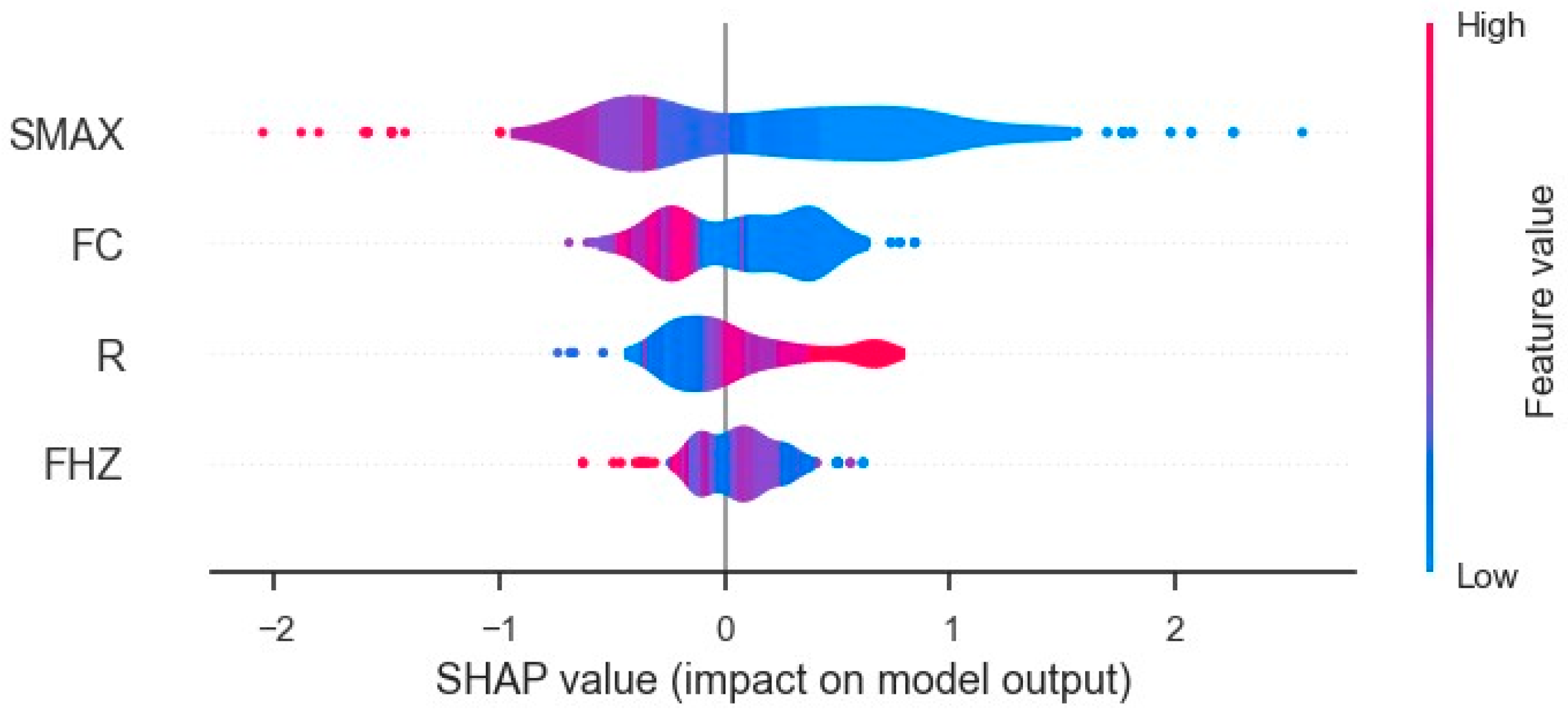
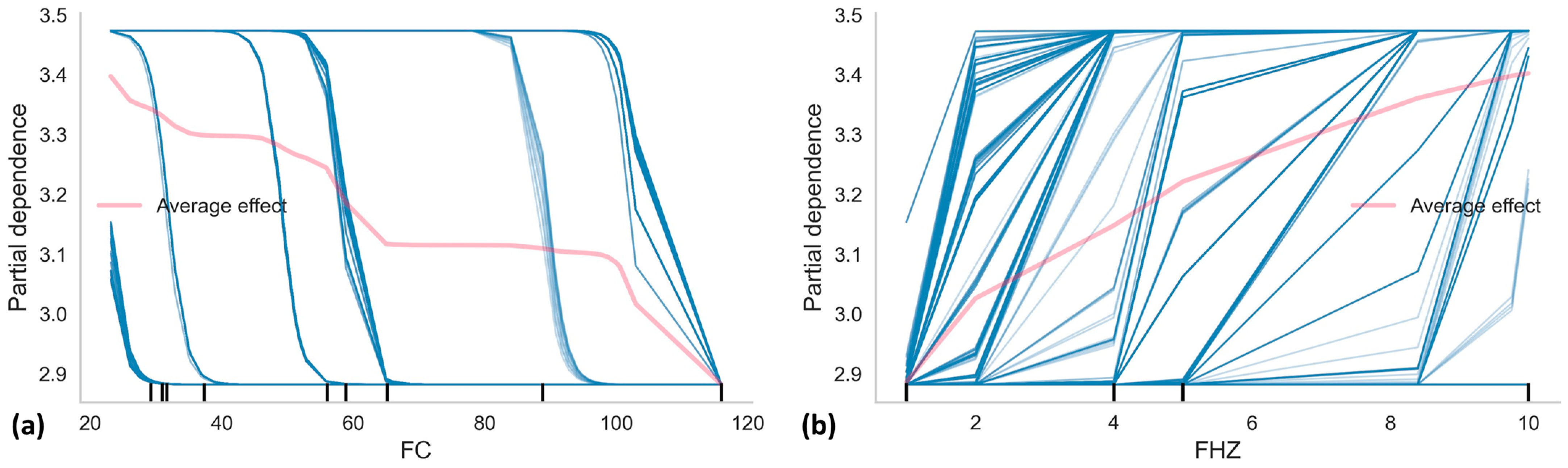
To assess the performance of all of the trained models, the mean absolute error (MAE), root-mean-square error (RMSE), coefficient of determination (R²), and mean absolute percentage error (MAPE) were calculated and evaluated.

The mean absolute error is a widely used metric in regression analysis to measure the absolute average magnitude of errors between predicted and actual values, as shown in Equation (11). It is advantageous when it is necessary to understand the average absolute difference between a prediction model and the observed values in a straightforward and interpretable manner.

$$MAE={\displaystyle \sum }_{i=1}^n{\displaystyle \frac{\left(y_i-t_i\right)}{n}}$$

(11)

where $t_i$ represents the observed values, $y_i$ represents the model outputs, and n is the amount of data samples evaluated.

As presented in Equation (12), the root-mean-square error calculates the average size of the errors, giving more weight to larger errors. This makes it particularly suitable for circumstances where large errors are more critical or destructive. The RMSE is useful because it quantifies the average prediction error and highlights the importance of significant errors by squaring the differences.

$$RMSE=\sqrt{{\displaystyle \sum }_{i=1}^n{\displaystyle \frac{{\left(y_i-t_i\right)}^2}{n}}}$$

(12)

The determination coefficient, presented in Equation (13), and sometimes known as R-squared, is a statistic used in regression analysis to assess how well a regression model fits the observed data. The R-squared (R²) indicates the proportion of variance in the dependent variable that the model’s independent variables can explain.

$$R^2={\left({\displaystyle \frac{{{\displaystyle \sum }}_{i=0}^{I-1}\left(t_i-\overline{t}\right)\left(y_i-\overline{y}\right)}{\sqrt{{{\displaystyle \sum }}_{i=0}^{I-1}{\left(t_i-\overline{t}\right)}^2{\left(y_i-\overline{y}\right)}^2}}}\right)}^2$$

(13)

Equation (14) presents the mean absolute percentage error in percentage terms, making it simple to understand. Compared to other error metrics, such as MSE or RMSE, MAPE is less sensitive to outliers. It provides a more balanced perspective on forecast accuracy, particularly in cases where high values may significantly influence other error measures.

$$MAPE={\displaystyle \frac{1}{n}}{\displaystyle \sum }_{i=1}^n\left|{\displaystyle \frac{t_i-y_i}{t_i}}\right|$$

(14)

2.5. SHAP Analysis

This study adopted SHAP (Shapley Additive Explanations) analysis as a method to enhance the interpretability of machine learning models. While such models are powerful in capturing nonlinear relationships and delivering robust predictive performance, they are often criticized for their black-box nature, which limits the understanding of how individual input features influence the output.

To address this issue, SHAP provides a comprehensive approach that quantifies the individual contribution of each input variable to the model’s prediction. This enables a detailed assessment of feature importance, allowing researchers to identify which variables have a significant impact on the outcome.

As highlighted by Mangalathu et al. [40], SHAP enhances models’ transparency by offering intuitive explanations of complex predictive behavior. According to Huo et al. [66], this method estimates the effect of each variable by observing how changes in its value influence the prediction, while keeping the other variables constant. Features that cause greater variation in output are considered to be more important.

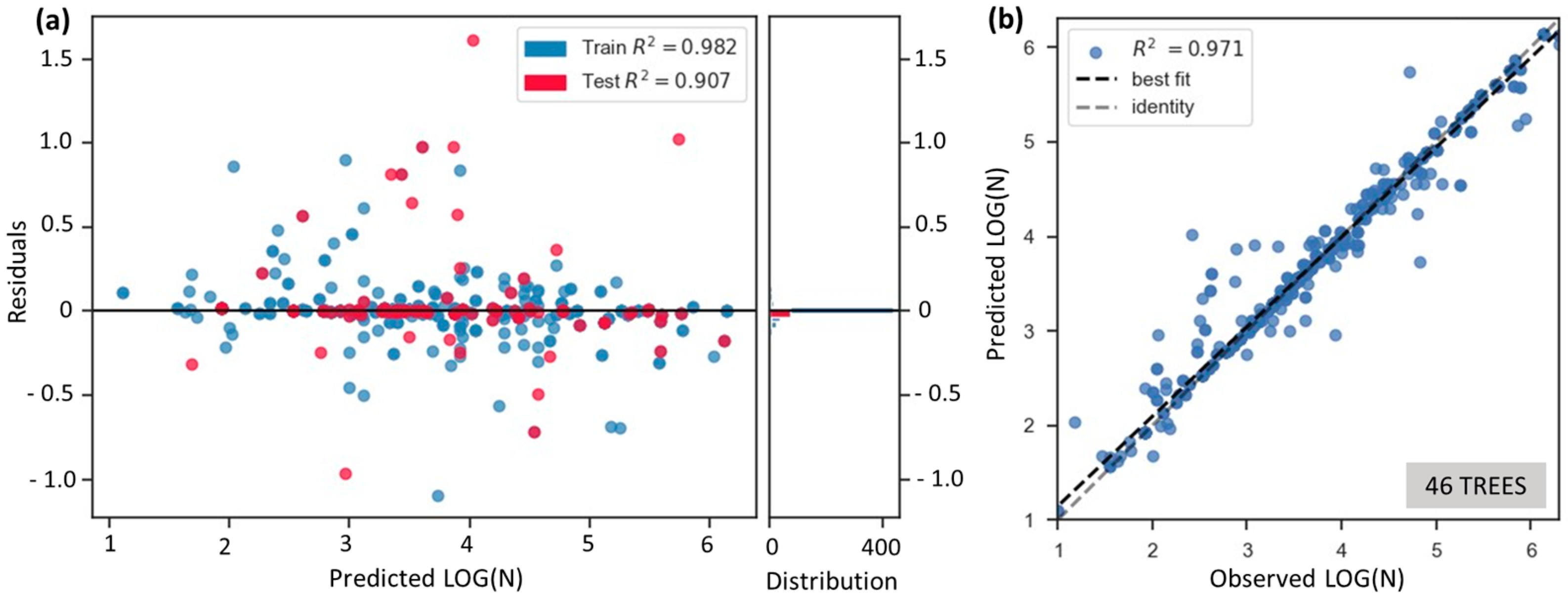
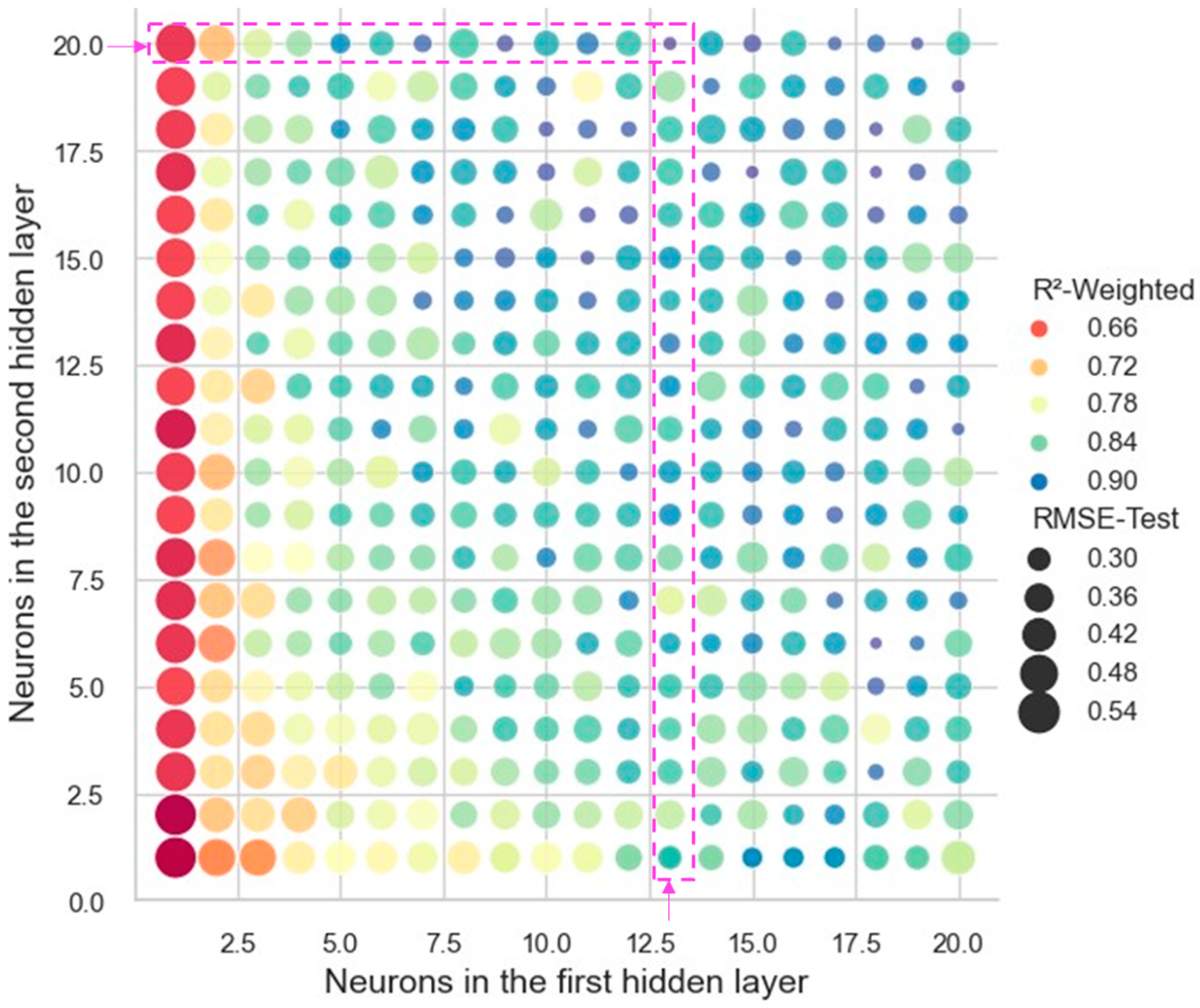
3. Results and Discussion

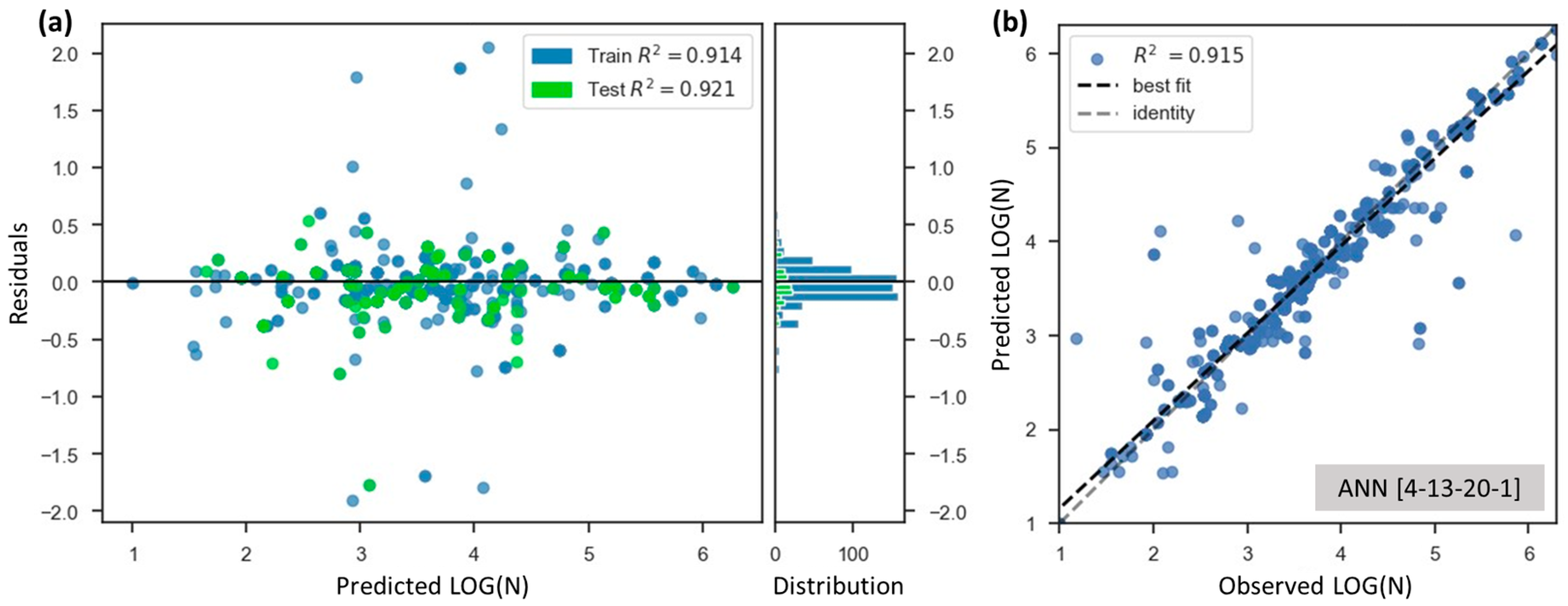
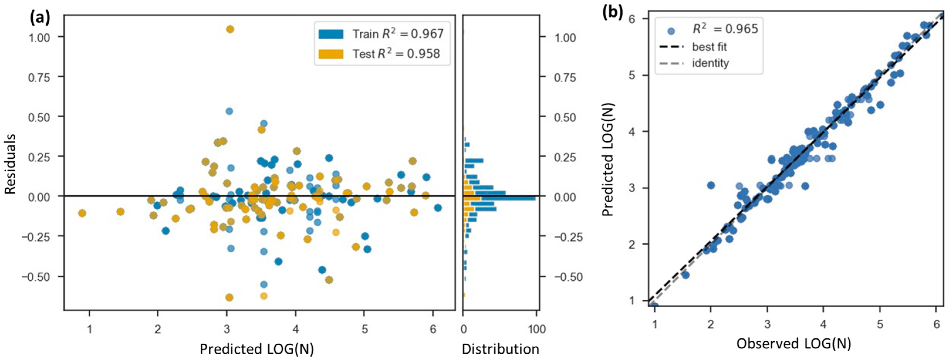
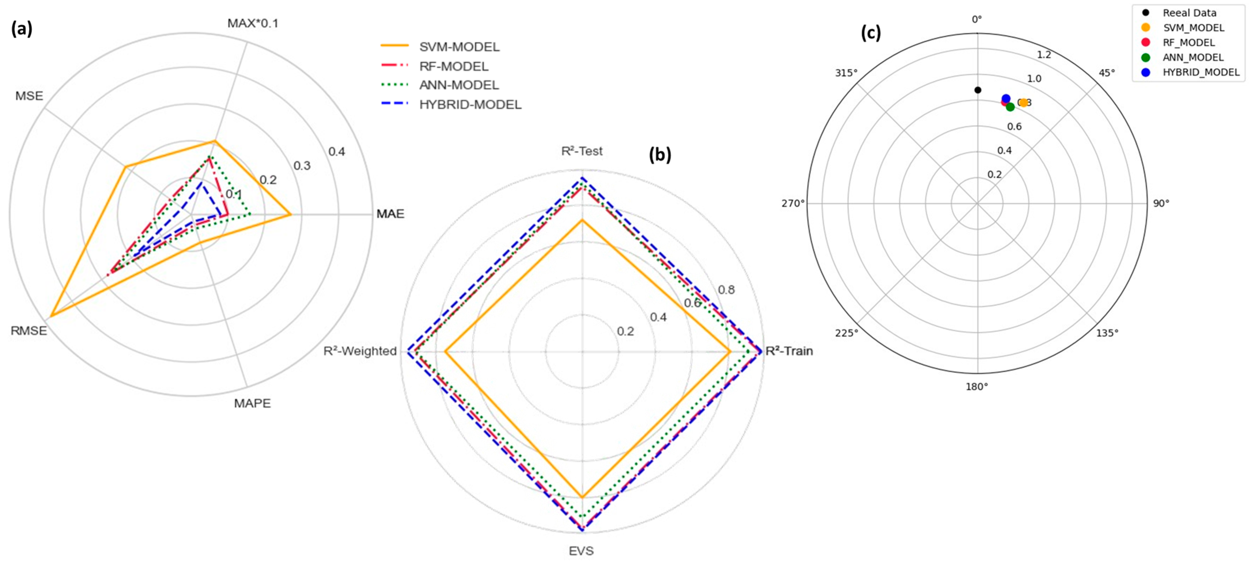
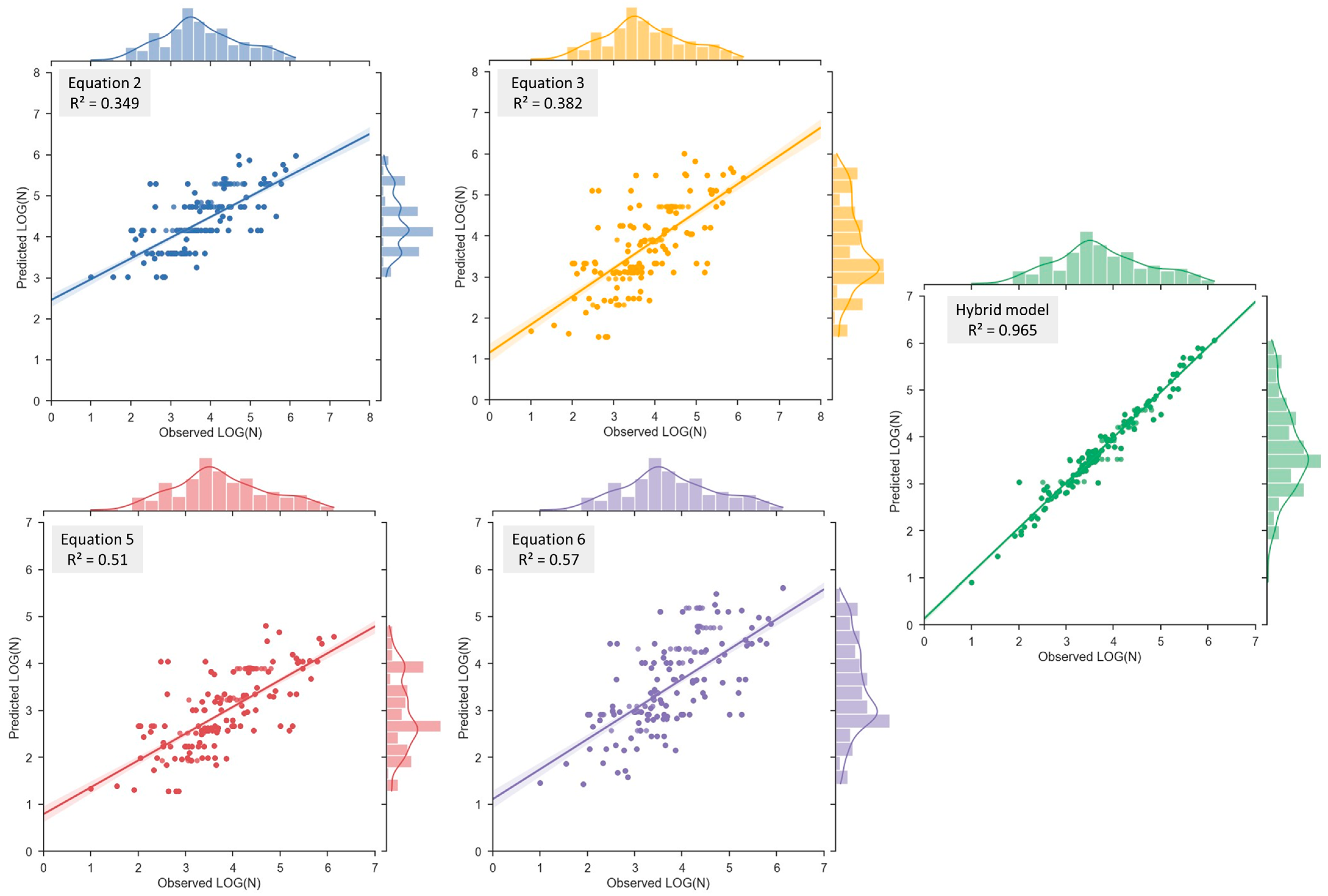
3.1. Models’ Performance

Initially, the performance of the individual machine learning techniques—Support Vector Machines (SVMs), Random Forest (RF), and Artificial Neural Networks (ANNs)—will be discussed separately. Subsequently, the performance of the proposed hybrid ensemble model, created using the stacking fusion strategy [68,73,74,90], will be examined. A SHAP analysis and comparison with other models from the literature were conducted to assess the model’s applicability and performance.

A strategy was employed to simplify and standardize the evaluation process to identify the best-performing base learning models for composing the hybrid predictor. For this purpose, a performance metric named $R_{WEIGHTED}^2$ (Equation (15)) was employed, integrating the training and testing performance. This metric was calculated by assigning a weight of 40% to $R_{TRAIN}^2$ and 60% to $R_{TEST}^2$, reflecting the importance of generalization performance when selecting the best-performing models. The decision to prioritize testing performance (60%) over training performance (40%) was based on the understanding that high training accuracy alone may indicate overfitting, compromising the model’s predictive ability on new, unseen data. By giving greater emphasis to the $R_{TEST}^2$ value, the $R_{WEIGHTED}^2$ metric promotes the selection of networks with the best generalization.

$$R_{WEIGHTED}^2=0.4R_{TRAIN}^2+0.6R_{TEST}^2$$

(15)

where $R_{TRAIN}^2$ is the determination coefficient achieved during the training phase, while $R_{TEST}^2$ is the determination coefficient calculated in the test phase.

Considering the results obtained during the training of the Support Vector Machine (SVM) base models, Figure 7 illustrates the variation in the determination coefficient (R²) as a function of the regularization parameter (C), evaluated for both polynomial and radial basis function (RBF) kernels. It is evident from the figure that the RBF kernel consistently outperformed the polynomial kernel across all tested values of C. Specifically, the R² values for the RBF kernel were significantly higher, indicating superior predictive performance and better generalization capability compared to the polynomial kernel. Moreover, as the regularization parameter increased, the performance of the SVM with the RBF kernel stabilized around a maximum value, reaching approximately 0.80 for the training data and around 0.72 for the test data, demonstrating good stability and generalization.

In contrast, the polynomial kernel showed notably lower R² values, remaining relatively stable and lower than 0.65. This outcome highlights the limited capability of the polynomial kernel to model the complexity and nonlinear characteristics inherent to predicting concrete’s fatigue life based on the input parameters used. Therefore, based on these observations, the RBF kernel was selected for further development of the hybrid ensemble model, due to its significantly superior performance, robustness, and ability to capture the nonlinear relationships present in the dataset.

The best-performing SVM model identified here utilized the radial basis function (RBF) kernel with a regularization parameter (C) equal to 900. The performance of this optimized SVM is presented in Figure 8, which includes both residual and dispersion plots. The residual plot (Figure 8a) shows that the residuals are relatively randomly distributed around the zero line, without trends or systematic patterns. Additionally, the training and test sets exhibited median determination coefficient (R²) values of 0.816 and 0.729, respectively, indicating the selected SVM model’s good predictive capability and reasonable generalization ability. The dispersion plot (Figure 8b) indicates a median linear correlation between the predicted and observed values, achieving an overall R² of 0.804. The MAPE was 8.05%, with an MAE of 0.274.

Continuing with the analysis of the base models, Figure 9 illustrates the performance obtained using Random Forest (RF) regression, where different split criteria—squared error, absolute error, Friedman mean squared error, and Poisson—were evaluated with varying numbers of decision trees (ranging from 2 to 100). The plot demonstrates that all of the criteria showed a rapid initial improvement in performance (R²) as the number of trees increased, stabilizing after approximately 20 trees were considered. Among the tested criteria, all of the error criteria demonstrated good performance in training (R² above 0.98). However, when analyzing the generalization capacity, the absolute error performed better, with stable values for both the weighted and test datasets (R² above 0.90), indicating an excellent generalization capability.

The best-performing RF base model, as defined by the absolute error criterion, consisted of 46 trees, and its performance is presented in Figure 10. The residual plot (Figure 10a) confirms the suitability of this model, with the residuals randomly dispersed around zero. This indicates the absence of clear patterns or bias, which is indicative of an adequate fit. The determination coefficient (R²) also achieved values of 0.982 for training and 0.907 for testing, reflecting a good, accurate, and generalizable model.

Furthermore, the regression plot (Figure 10b) displays an excellent correlation between the predicted and observed values, achieving a general R² of 0.971. The MAPE was 3.36%, with an MAE of 0.105. The predictions closely align with the identity line, further confirming the good performance of this selected RF model.

Figure 11 provides an overview of the performance of the ANNs trained with 400 distinct topologies. The weighted determination coefficient ($R_{WEIGHTED}^2$), represented by color intensity, and the root-mean-square error for the test set (RMSE-Test), indicated by bubble size, depict how network performance varies with the number of neurons in each hidden layer. The plot reveals that ANNs with fewer neurons, especially in the first hidden layer, exhibited lower R² values and larger RMSEs, highlighting inadequate complexity to model the underlying relationships. However, as the number of neurons increased, particularly beyond 10 neurons in each hidden layer, performance markedly improved, as reflected by higher $R_{WEIGHTED}^2$ and smaller RMSE values.

Based on Figure 11, the ANN model exhibiting the best performance was identified as having the [4-13-20-1] topology (identified with the purple dashed box), comprising four input neurons, thirteen neurons in the first hidden layer, twenty neurons in the second hidden layer, and a single output neuron. Figure 12 indicates the performance of the ANN [4-13-20-1]. The residual plot (Figure 12a) shows randomly dispersed residuals centered around zero, indicating no evident systematic bias, which supports good homoscedasticity and an appropriate model. The training and test sets yielded excellent R² values of 0.914 and 0.921, respectively, indicating high accuracy and good generalization capabilities. The dispersion plot (Figure 12b) confirms this performance, achieving an overall R² of 0.915, with the predicted values closely aligned with the identity line. The MAPE was 4.89%, with an MAE of 0.168. The observed points consistently follow the best-fit line, validating the ANN model’s capability to effectively capture and predict complex, nonlinear patterns within the data.

After defining the optimal base models (SVM with an RBF kernel and C = 900, RF with 46 trees and the squared error split criterion, and ANN with the topology [4-13-20-1]), the next step involved building the hybrid ensemble model using the stacking fusion strategy [90]. This strategy was implemented by applying a linear regression model based on the least squares method, where the predictions from the three selected base models were used as inputs. Equation (16) represents the final formulation of the hybrid model, where the output fatigue life prediction, expressed as LOG(N), is calculated as a weighted combination of the individual model predictions:

$$LOG\left(N\right)=0.08LOG{\left(N\right)}_{SVM}+1.03LOG{\left(N\right)}_{RF}-0.13{\beta }_{ANN}LOG{\left(N\right)}_{ANN}-0.046$$

(16)

The performance of the hybrid model is indicated in Figure 13. The residual plot (Figure 13a) shows a very tight and symmetric distribution of errors around the zero line for both the training and test sets, with minimal dispersion and no evident pattern, indicating high consistency and low bias. The determination coefficients obtained were R² = 0.967 for training and R² = 0.958 for testing, confirming the hybrid model’s strong predictive performance and excellent generalization capability. The regression plot (Figure 13b) emphasizes this, with a global R² of 0.965, and the predicted values align closely with the identity line. The MAPE was 2.39%, with an MAE of 0.084. This result demonstrates that the stacking ensemble approach effectively combines the strengths of each model while mitigating their weaknesses.

Figure 14a,b presents a comparative analysis of the base models (SVM, RF, and ANN) against the hybrid ensemble model using two radar plots, while Figure 14c presents the Taylor diagram plots. The radar chart in Figure 14a displays key error metrics, including the mean absolute error (MAE), mean squared error (MSE), root-mean-square error (RMSE), mean absolute percentage error (MAPE), and the maximum error divided by 10 (MAX×0.1). The radar chart in Figure 14b displays the determination coefficients (R²) for both the training and test datasets, along with the $R_{WEIGHTED}^2$ and the explained variance score (EVS).

The hybrid model outperformed all of the base models across every metric. The hybrid model achieved a low value of 0.19 (in LOG(Cycles)) for the RMSE, which is significantly lower than the RMSE values of the SVM (0.47), RF (0.28), and ANN (0.26) models, confirming the hybrid model’s superior ability to predict the R². The MAE and MSE values also followed this trend, with the hybrid model occupying the smallest area in the radar chart, indicating the lowest absolute and squared errors among the models.

The hybrid model also excelled in terms of generalization and overall predictive capability, achieving an overall R² of 0.965. Notably, the R² values were 0.967 for training and 0.956 for testing. These values are higher than those of the ANN model (0.914 train/0.921 test), the RF model (0.982 train/0.907 test), and the SVM model (0.816 train/0.729 test), indicating better alignment between the predicted and actual values across both training and unseen data.

Figure 14c shows that all of the base models (SVM, RF, ANN) and the hybrid model exhibit strong correlations with reference data, as indicated by their proximity to the angle of 0°, corresponding to a correlation close to 1.0. However, the differences in radial distance highlight variations in the standard deviation of their predictions relative to the observed data. The Random Forest and Artificial Neural Network models slightly overestimate the standard deviation, positioning themselves further away from the reference arc. In contrast, the SVM model aligns more closely regarding the standard deviation, but it exhibits a slightly lower correlation than the hybrid model.

Most notably, the hybrid model, represented in blue, is the closest to the reference point in both angular and radial coordinates. This indicates that it achieves a higher correlation and maintains a standard deviation that is more consistent with the observed data, reflecting better calibration. This overall proximity to the reference point confirms the hybrid model’s superiority in capturing the underlying distribution and trends of the dataset, effectively integrating the strengths of the base learners.

These findings indicate that while the base models individually offer reasonable performance, the hybrid model, with a stacking fusion strategy, demonstrates a better balance between correlation and variability representation, making it the most suitable approach for predicting the fatigue life of concrete.

3.2. AI4SNConcrete App with Graphical Interface and Model Analysis

Figure 15 presents a performance comparison between the proposed model and empirical formulations from the literature (Equations (2), (3), (5), and (6)). These equations were selected based on their compatibility with the input parameters available in the dataset, such as the maximum stress ratio, compressive strength, and stress ratio. The performance of each model was evaluated in terms of the coefficient of determination (R²), which is shown in the respective plots.

Equations (2) and (3), derived from the classical Wöhler approach, show the lowest predictive capability, with R² values of 0.349 and 0.382, respectively. These formulations typically incorporate only two input variables: the stress level and compressive strength, and do not account for the nonlinear effects of load frequency or stress ratio. As a result, they tend to oversimplify the fatigue phenomenon and fail to capture the full variability observed in the experimental data.

Equation (5), described in the Dutch National Code NEN 6723:2009 [12] recommendations, incorporates the stress ratio R and the design and reference strengths. It performs slightly better than the previous equations, achieving an R² of 0.51. Equation (6), as described in the fib Model Code [8], which includes parameters such as the maximum and minimum stress ratios, achieved the best performance among the formulations from the literature, with an R² value of 0.57. Nonetheless, all of these models presented performances lower than that of the hybrid model. The hybrid model achieved an R² of 0.965, indicating a tight distribution of the predicted values along the identity line, with minimal dispersion. This indicates its superior ability to generalize and capture complex, nonlinear interactions among the input parameters.

Abambres and Lantsoght [53] compared the performances of machine learning models and analytical formulations to assess the fatigue behavior of concrete subjected to compressive cyclic loads using Artificial Neural Networks (ANNs). The proposed model demonstrated superior predictive performance, with a mean tested-to-predicted ratio of 1.00 and a coefficient of variation of 1.7%. This performance was superior to that of existing code-based expressions, particularly Equations (5) and (6) [8,12]. Among these current code methods, the fib Model Code [8] showed the best performance, with an average tested-to-predicted stress ratio of 1.37 and a coefficient of variation of 20.5%.

The findings highlight a key limitation of analytical models: the lack of consideration for loading frequency. None of the empirical equations explicitly accounts for the loading frequency, even though it is widely recognized that fatigue performance is highly sensitive to cyclic frequency, especially at higher rates (e.g., 1–10 Hz, as in the dataset used here). The hybrid model, on the other hand, directly incorporates frequency as an input, allowing for more accurate predictions under real loading conditions. This is particularly valuable for the design and safety assessment of structural elements subjected to dynamic or repetitive loading, such as bridge decks, industrial floors, and railway sleepers.

A key consideration in evaluating the applicability of the proposed hybrid model is the definition of its domain of validity. As with any data-driven model, its predictive reliability is inherently limited to the range of values represented in the training dataset. The ranges observed in the dataset define the valid domain for model applications, which includes compressive strength values from 23.10 MPa to 116.00 MPa, SMAX values between 0.62 and 0.95, R values ranging from 0.01 to 0.50, and frequencies between 1.00 Hz and 10.00 Hz. Predictions made outside these intervals should be interpreted cautiously, as the model was neither trained nor validated under such conditions.

Figure 16 presents the SHAP summary plot, where each point represents the SHAP value for a particular prediction and feature. The color gradient indicates the actual feature value, ranging from low (blue) to high (red). At the same time, the horizontal axis displays the SHAP value, reflecting each feature’s impact on the predicted output (LOG(N)). SMAX exhibited the highest influence on the model’s predictions among the analyzed features. Higher SMAX values consistently led to lower predicted fatigue life. In contrast, lower SMAX values (indicated in blue) were associated with increased fatigue life, in agreement with well-established principles of fatigue mechanics [19,86,91].

Compressive strength (FC) emerged as the second-most influential variable after SMAX. Higher compressive strengths tended to increase the predicted fatigue life, indicating that stronger concretes can sustain higher stresses over more load cycles due to their improved mechanical properties. The stress ratio (R) also demonstrated a moderate impact on the predictions, with its influence depending on the interaction with other input features. Meanwhile, the loading frequency (FHZ) exhibited a noticeable yet moderate effect on the model outputs. Its SHAP values suggest that frequency remains an important parameter, reinforcing findings from experimental studies that emphasize the effect of loading rate on fatigue behavior [18,19,77].

Given the relevance of compressive strength (FC) and loading frequency (FHZ) highlighted in the SHAP analysis, additional investigations were conducted to further explore their relationships with the predicted fatigue life. Thus, Partial Dependence Plots (PDPs) and Individual Conditional Expectation (ICE) curves were generated for these variables, as shown in Figure 17. Notably, PDPs and ICE plots were not constructed for SMAX and R, as their strong influence on fatigue behavior is already well documented in the literature, making their critical role self-evident.

For loading frequency (Figure 17a), the PDP analysis reveals a clear and consistent trend: as FHZ increases from 1 Hz to 10 Hz, the predicted fatigue life (LOG(N)) also increases. The dashed line, representing the PDP, captures the average effect across the dataset, showing that higher loading frequencies are associated with extended fatigue life. This result is physically interpretable, as higher frequencies typically reduce the exposure time per load cycle, thereby moderating damage accumulation mechanisms. The ICE curves reinforce this observation, illustrating that individual instances predominantly follow the same increasing trend, which indicates a stable and generalized influence of frequency across the data.

In contrast, the analysis of compressive strength (Figure 17b) presents an intriguing trend. The PDP suggests a slight decrease in the predicted LOG(N) as FC increases. While this behavior may initially appear counterintuitive, it is consistent with experimental evidence indicating that high-strength concretes, despite their superior performance under static loading, tend to exhibit increased brittleness and reduced energy dissipation capacity under cyclic compressive stresses. The ICE curves support this interpretation by showing a coherent trend across individual predictions, reinforcing that although high compressive strength improves the ultimate capacity, it may also adversely affect fatigue endurance due to the material’s inherent fragility under repetitive loading.

Together, these findings emphasize the need for predictive models of fatigue life—or S-N curves for cyclic compression in concrete—to account for mechanical resistance properties (such as compressive strength) and loading characteristics (such as frequency). Neglecting either parameter may limit the model’s generalization ability across different concrete types and loading scenarios. The model developed in this study proved capable of capturing these nonlinear and interacting effects, reinforcing its applicability as a robust and interpretable tool for fatigue analysis in reinforced concrete design and durability assessments.

To promote the practical application of the proposed model and facilitate its adoption by engineers and practitioners, a user-friendly web-based interface, AI4SNConcrete, was developed and is now publicly available on the research group’s website (https://ai4snconcrete.dasmae.com/, accessed on 20 April 2025). This application allows users to easily generate S-N curves to evaluate the fatigue life of concrete elements subjected to cyclic compressive loading. The user must input three key parameters to use the tool: the material’s compressive strength, the ratio between the minimum and maximum applied stress, and the loading frequency. Based on these inputs, the application returns red points representing the predicted LOG(N) values for different maximum stress-to-strength ratios. A regression line is then fitted to these points, accompanied by an error margin of ±4%, forming a complete S-N curve that can be directly used for fatigue design and assessment. Figure 18 illustrates the web application’s interface, highlighting its simplicity and usability. This platform bridges the gap between machine learning and engineering practice, offering an accessible means of incorporating data-driven fatigue predictions into structural analysis workflows.

4. Conclusions

This study proposed a hybrid predictive model for estimating the fatigue life (LOG(N)) of plain concrete under cyclic compressive loading by integrating Support Vector Regression (SVR), Random Forest (RF), and Artificial Neural Network (ANN) models through a stacking ensemble strategy. This approach successfully addressed key limitations observed in conventional empirical models, offering higher predictive accuracy and better generalization capacity. Through the analysis conducted here, several important contributions and results can be highlighted:

• Development of a highly accurate stacking-based hybrid model combining SVR, RF, and ANN approaches to predict the fatigue life of plain concrete, achieving R² = 0.965 and RMSE = 0.19.
• Identification that only four input variables—compressive strength (FC), maximum stress ratio (SMAX), stress ratio (R), and loading frequency (FHZ)—are sufficient to model concrete’s fatigue behavior accurately.
• Applying SHAP analysis to interpret the model, confirming SMAX as the most influential variable, followed by FC, with R and FHZ also playing significant, albeit secondary, roles.
• Generation of Partial Dependence Plots (PDPs) and Individual Conditional Expectation (ICE) curves for FC and FHZ, providing a detailed and physically interpretable understanding of how these features affect the predicted fatigue life.
• Developing and publicly releasing a user-friendly web application based on the proposed hybrid model, allowing engineers and practitioners to easily generate S-N curves for plain concrete under cyclic loading. This tool simplifies the application of machine learning techniques in practice and can be accessed at https://ai4snconcrete.dasmae.com/ (accessed on 20 April 2025).

The interpretability techniques applied here, including SHAP values and PDP/ICE curves, not only validated the physical consistency of the model’s predictions but also enhanced our understanding of the relative importance of the inputs considered. The compressive strength (FC) and loading frequency (FHZ) were particularly influential, highlighting the necessity of carefully considering these parameters in fatigue durability models for concrete structures.

However, it is important to recognize some limitations. The predictive applicability of the model is restricted to the ranges covered by the training dataset: compressive strengths between 23.10 MPa and 116.00 MPa, maximum stress ratios between 0.62 and 0.95, stress ratios between 0.01 and 0.50, and loading frequencies between 1.00 Hz and 10.00 Hz. Extrapolations outside these domains may not maintain the same reliability. Furthermore, the model was trained using data for plain concrete only. Therefore, it does not account for the behavior of fiber-reinforced concretes or concretes subjected to aggressive environmental exposures.

Future work should expand the database to incorporate a wider range of concrete types, loading patterns (including variable amplitude fatigue), and exposure conditions (such as freeze–thaw cycles and chemical attacks). Additionally, integrating uncertainty quantification methods into the predictions would provide users with confidence intervals, supporting safer engineering decisions. Expanding the web application’s functionalities to accommodate different concrete classes, environmental exposures, and loading protocols would further enhance its practical relevance for fatigue durability assessments in structural engineering.

References

1. Clemmer, H.F. Fatigue of Concrete. Proc. Am. Soc. Test. Mater. 1922, 22, 408–419. [Google Scholar]
2. Hsu, T.T.C. Fatigue of Plain Concrete. ACI J. Proc. 1981, 78, 292–305. [Google Scholar] [CrossRef]
3. Do, M.; Chaallal, O.; Aïtcin, P. Fatigue Behavior of High-Performance Concrete. J. Mater. Civ. Eng. 1993, 5, 96–111. [Google Scholar] [CrossRef]
4. Kolluru, S.V.; O’Neil, E.F.; Popovics, J.S.; Shah, S.P. Crack Propagation in Flexural Fatigue of Concrete. J. Eng. Mech. 2000, 126, 891–898. [Google Scholar] [CrossRef]
5. Subramaniam, K.V.; Shah, S.P. Biaxial Tension Fatigue Response of Concrete. Cem. Concr. Compos. 2003, 25, 617–623. [Google Scholar] [CrossRef]
6. Cornellissen, H.A.W. Fatigue Failure of Concrete in Tension. Heron 1984, 29, 2–67. [Google Scholar]
7. Callister, W.D., Jr.; Rethwisch, D.G. Materials Science and Engineering: An Introduction, 10th ed.; Wiley: Hoboken, NJ, USA, 2017. [Google Scholar]
8. Fédération Internationale du Béton. Model Code 2010: Final Draft; Fib Bulletin 65-66. International Federation for Structural, 2012. Available online: https://www.fib-international.org/publications/fib-bulletins/model-code-2010-final-draft,-volume-1-detail.html (accessed on 5 April 2025).
9. Raithby, K.D.; Galloway, J.W. Effects of Moisture Condition, Age, and Rate of Loading on Fatigue of Plain Concrete. In Proceedings of the ABELES Symposium: Fatigue of Concrete; ACI Publication: Farmington Hills, MI, USA, 1974; pp. 15–34. [Google Scholar]
10. Sparks, P.R. The Influence of Rate of Loading and Material Variability on the Fatigue Characteristics of Concrete. ACI J. 1982, 75, 331–342. [Google Scholar]
11. Tepfers, R.; Kutti, T. Fatigue Strength of Plain, Ordinary and Lightweight Concrete. ACI J. 1979, 76, 635–652. [Google Scholar]
12. Code Committee 351 001. Technical Foundations for Structures. In Regulations for Concrete-Bridges-Structural Requirements and Calculation Methods, NEN 6723:2009; Nederlands Normalisatie Instituut: Gouda, The Netherlands, 2009. [Google Scholar]
13. Lee, M.K.; Barr, B.I.G. An Overview of the Fatigue Behaviour of Plain and Fibre Reinforced Concrete. Cem. Concr. Compos. 2004, 26, 299–305. [Google Scholar] [CrossRef]
14. Ortega, J.J.; Ruiz, G.; Yu, R.C.; Afanador-García, N.; Tarifa, M.; Poveda, E.; Zhang, X.; Evangelista, F. Number of Tests and Corresponding Error in Concrete Fatigue. Int. J. Fatigue 2018, 116, 210–219. [Google Scholar] [CrossRef]
15. Son, J.; Yang, S. A New Approach to Machine Learning Model Development for Prediction of Concrete Fatigue Life under Uniaxial Compression. Appl. Sci. 2022, 12, 9766. [Google Scholar] [CrossRef]
16. Lee, H.; Lee, H.-S.; Suraneni, P. Evaluation of Carbonation Progress Using AIJ Model, FEM Analysis, and Machine Learning Algorithms. Constr. Build. Mater. 2020, 259, 119703. [Google Scholar] [CrossRef]
17. Felix, E.F.; Carrazedo, R.; Possan, E. Vida Útil à Fadiga Do Concreto: Estudo Experimental Da Influência Das Condições de Carregamento e Da Resistência Do Material. Rev. ALCONPAT 2022, 12, 1–15. [Google Scholar] [CrossRef]
18. Felix, E.F.; Carrazedo, R.; Possan, E. Análise Experimental Da Vida Útil à Fadiga de Concretos Submetidos à Compressão Cíclica de Baixa Frequência. Matéria 2022, 27, e202145017. [Google Scholar] [CrossRef]
19. Medeiros, A.; Zhang, X.; Ruiz, G.; Yu, R.C.; Velasco, M.d.S.L. Effect of the Loading Frequency on the Compressive Fatigue Behavior of Plain and Fiber Reinforced Concrete. Int. J. Fatigue 2015, 70, 342–350. [Google Scholar] [CrossRef]
20. Sain, T.; Chandrakishen, J. Residual Fatigue Strength Assessment of Concrete Considering Tension Softening Behavior. Int. J. Fatigue 2007, 29, 2138–2148. [Google Scholar] [CrossRef]
21. Liang, J.; Ding, Z.; Li, J. A Probabilistic Analyzed Method for Concrete Fatigue Life. Probabilistic Eng. Mech. 2017, 49, 13–21. [Google Scholar] [CrossRef]
22. Li, J.; Gao, R. Fatigue Reliability Analysis of Concrete Structures Based on Physical Synthesis Method. Probabilistic Eng. Mech. 2019, 56, 14–26. [Google Scholar] [CrossRef]
23. Cui, K.; Xu, L.; Li, L.; Chi, Y. Mechanical Performance of Steel-Polypropylene Hybrid Fiber Reinforced Concrete Subject to Uniaxial Constant-Amplitude Cyclic Compression: Fatigue Behavior and Unified Fatigue Equation. Compos. Struct. 2023, 311, 116795. [Google Scholar] [CrossRef]
24. Zhang, W.; Lee, D.; Lee, J.; Lee, C. Residual Strength of Concrete Subjected to Fatigue Based on Machine Learning Technique. Struct. Concr. 2022, 23, 2274–2287. [Google Scholar] [CrossRef]
25. Shi, J.; Zhang, W.; Zhao, Y. ANN Prediction Model of Concrete Fatigue Life Based on GRW-DBA Data Augmentation. Appl. Sci. 2023, 13, 1227. [Google Scholar] [CrossRef]
26. Adeli, H.; Yeh, C. Perceptron Learning in Engineering Design. Comput.-Aided Civ. Infrastruct. Eng. 1989, 4, 247–256. [Google Scholar] [CrossRef]
27. Williams, T.P.; Gucunski, N. Neural Networks for Backcalculation of Moduli from SASW Test. J. Comput. Civ. Eng. 1995, 9, 1–8. [Google Scholar] [CrossRef]
28. Goh, A.T.C. Neural Networks for Evaluating CPT Calibration Chamber Test Data. Comput.-Aided Civ. Infrastruct. Eng. 1995, 10, 147–151. [Google Scholar] [CrossRef]
29. Bonini Neto, A.; dos Santos Batista Bonini, C.; Santos Bisi, B.; Rodrigues dos Reis, A.; Sommaggio Coletta, L.F. Artificial Neural Network for Classification and Analysis of Degraded Soils. IEEE Lat. Am. Trans. 2017, 15, 503–509. [Google Scholar] [CrossRef]
30. Xie, J.; Huang, J.; Zeng, C.; Huang, S.; Burton, G.J. A Generic Framework for Geotechnical Subsurface Modeling with Machine Learning. J. Rock. Mech. Geotech. Eng. 2022, 14, 1366–1379. [Google Scholar] [CrossRef]
31. Puri, N.; Prasad, H.D.; Jain, A. Prediction of Geotechnical Parameters Using Machine Learning Techniques. Procedia Comput. Sci. 2018, 125, 509–517. [Google Scholar] [CrossRef]
32. Lin, S.; Liang, Z.; Zhao, S.; Dong, M.; Guo, H.; Zheng, H. A Comprehensive Evaluation of Ensemble Machine Learning in Geotechnical Stability Analysis and Explainability. Int. J. Mech. Mater. Des. 2024, 20, 331–352. [Google Scholar] [CrossRef]
33. Zhang, W.; Gu, X.; Hong, L.; Han, L.; Wang, L. Comprehensive Review of Machine Learning in Geotechnical Reliability Analysis: Algorithms, Applications and Further Challenges. Appl. Soft Comput. 2023, 136, 110066. [Google Scholar] [CrossRef]
34. Jenkins, W.M. A Neural Network for Structural Re-Analysis. Comput. Struct. 1999, 72, 687–698. [Google Scholar] [CrossRef]
35. Babiker, S.A.; Adam, F.M.; Mohamed, A.E. Design Optimization of Reinforced Concrete Beams Using Concrete Beams Using Artificial Neural Network. Green. Bookee 2012, 1, 07–13. [Google Scholar]
36. Ge, K.; Wang, C.; Guo, Y.T.; Tang, Y.S.; Hu, Z.Z.; Chen, H.B. Fine-Tuning Vision Foundation Model for Crack Segmentation in Civil Infrastructures. Constr. Build. Mater. 2024, 431, 136573. [Google Scholar] [CrossRef]
37. Félix, E.F.; Falcão, I.d.S.; dos Santos, L.G.; Carrazedo, R.; Possan, E. A Monte Carlo-Based Approach to Assess the Reinforcement Depassivation Probability of RC Structures: Simulation and Analysis. Buildings 2023, 13, 993. [Google Scholar] [CrossRef]
38. Felix, E.F.; Carrazedo, R. Análise Probabilística Da Vida Útil de Lajes de Concreto Armado Sujeitas à Corrosão Por Carbonatação via Simulação de Monte Carlo. Matéria 2021, 26, e13043. [Google Scholar] [CrossRef]
39. Felix, E.F.; Lavinicki, B.M.; Bueno, T.L.G.T.; de Castro, T.C.C.; Cândido, R.A. Integrating Machine Learning and Monte Carlo Simulation for Probabilistic Assessment of Durability in RC Structures Affected by Carbonation-Induced Corrosion. J. Build. Pathol. Rehabil. 2024, 9, 143. [Google Scholar] [CrossRef]
40. Mangalathu, S.; Hwang, S.-H.; Jeon, J.-S. Failure Mode and Effects Analysis of RC Members Based on Machine-Learning-Based SHapley Additive ExPlanations (SHAP) Approach. Eng. Struct. 2020, 219, 110927. [Google Scholar] [CrossRef]
41. Li, G.; Luo, R.; Yu, D.-H. A Framework for Developing a Machine Learning-Based Finite Element Model for Structural Analysis. Comput. Struct. 2025, 307, 107617. [Google Scholar] [CrossRef]
42. Adeli, H. Advances in Design Optimization; Adeli, H., Ed.; CRC Press: Boca Raton, FL, USA, 1994; ISBN 9780429082245. [Google Scholar]
43. Al-Suhaili, R.H.S.; Ali, A.A.M.; Behaya, S.A.K. Artificial Neural Network Modeling for Dynamic Analysis of a Dam-Reservoir-Foundation System. Int. J. Eng. Res. Appl. 2014, 4, 10–32. [Google Scholar]
44. Ge, K.; Wang, C.; Guo, Y.-T.; Tang, Y.-S.; Fan, J.-S. A Multitask Fourier Transformer Network for Seismic Source Characterization Estimation From a Single-Station Waveform. IEEE Geosci. Remote Sens. Lett. 2024, 21, 1–5. [Google Scholar] [CrossRef]
45. Ge, K.; Guo, Y.T.; Wang, C.; Hu, Z.Z. AI-Based Prediction of Seismic Time-History Responses of RC Frame Structures Considering Varied Structural Parameters. J. Build. Eng. 2025, 106, 112643. [Google Scholar] [CrossRef]
46. Neves, A.C.; González, I.; Karoumi, R.; Leander, J. The Influence of Frequency Content on the Performance of Artificial Neural Network–Based Damage Detection Systems Tested on Numerical and Experimental Bridge Data. Struct. Health Monit. 2021, 20, 1331–1347. [Google Scholar] [CrossRef]
47. Gomes, G.F.; Mendez, Y.A.D.; da Silva Lopes Alexandrino, P.; da Cunha, S.S.; Ancelotti, A.C. A Review of Vibration Based Inverse Methods for Damage Detection and Identification in Mechanical Structures Using Optimization Algorithms and ANN. Arch. Comput. Methods Eng. 2019, 26, 883–897. [Google Scholar] [CrossRef]
48. Bakhary, N.; Hao, H.; Deeks, A.J. Damage Detection Using Artificial Neural Network with Consideration of Uncertainties. Eng. Struct. 2007, 29, 2806–2815. [Google Scholar] [CrossRef]
49. Jeyasehar, C.A.; Sumangala, K. Damage Assessment of Prestressed Concrete Beams Using Artificial Neural Network (ANN) Approach. Comput. Struct. 2006, 84, 1709–1718. [Google Scholar] [CrossRef]
50. Bonifácio, A.L.; Mendes, J.C.; Farage, M.C.R.; Barbosa, F.S.; Barbosa, C.B.; Beaucour, A.-L. Application of Support Vector Machine and Finite Element Method to Predict the Mechanical Properties of Concrete. Lat. Am. J. Solids Struct. 2019, 16, e205. [Google Scholar] [CrossRef]
51. Jueyendah, S.; Lezgy-Nazargah, M.; Eskandari-Naddaf, H.; Emamian, S.A. Predicting the Mechanical Properties of Cement Mortar Using the Support Vector Machine Approach. Constr. Build. Mater. 2021, 291, 123396. [Google Scholar] [CrossRef]
52. Saha, P.; Debnath, P.; Thomas, P. Prediction of Fresh and Hardened Properties of Self-Compacting Concrete Using Support Vector Regression Approach. Neural Comput. Appl. 2020, 32, 7995–8010. [Google Scholar] [CrossRef]
53. Abambres, M.; Lantsoght, E.O.L. Lantsoght ANN-Based Fatigue Strength of Concrete under Compression. Materials 2019, 12, 3787. [Google Scholar] [CrossRef]
54. Fathalla, E.; Tanaka, Y.; Maekawa, K. Remaining Fatigue Life Assessment of In-Service Road Bridge Decks Based upon Artificial Neural Networks. Eng. Struct. 2018, 171, 602–616. [Google Scholar] [CrossRef]
55. Rabin Gani, B.; Simon, K.M.; Bharati Raj, J. Development of Artificial Neural Network for the Fatigue Life Assessment of Self Compacting Concrete. In International Conference on Structural Engineering and Construction Management; Springer International Publishing: Cham, Switzerland, 2023; pp. 695–704. [Google Scholar]
56. Zheng, D.; Ozbayoglu, E.; Miska, S.Z.; Liu, Y.; Li, Y. Cement Sheath Fatigue Failure Prediction by ANN-Based Model. In Proceedings of the Offshore Technology Conference, Houston, TX, USA, 25 April 2022. [Google Scholar]
57. Al-Saraireh, M.A. Predicting Compressive Strength of Concrete with Fly Ash, Metakaolin and Silica Fume by Using Machine Learning Techniques. Lat. Am. J. Solids Struct. 2022, 19, e454. [Google Scholar] [CrossRef]
58. Endzhievskaya, I.G.; Endzhievskiy, A.S.; Galkin, M.A.; Molokeev, M.S. Machine Learning Methods in Assessing the Effect of Mixture Composition on the Physical and Mechanical Characteristics of Road Concrete. J. Build. Eng. 2023, 76, 107248. [Google Scholar] [CrossRef]
59. Khodaparasti, M.; Alijamaat, A.; Pouraminian, M. Prediction of the Concrete Compressive Strength Using Improved Random Forest Algorithm. J. Build. Pathol. Rehabil. 2023, 8, 92. [Google Scholar] [CrossRef]
60. Li, H.; Lin, J.; Lei, X.; Wei, T. Compressive Strength Prediction of Basalt Fiber Reinforced Concrete via Random Forest Algorithm. Mater. Today Commun. 2022, 30, 103117. [Google Scholar] [CrossRef]
61. Alabduljabbar, H.; Khan, K.; Awan, H.H.; Alyousef, R.; Mohamed, A.M.; Eldin, S.M. Modeling the Capacity of Engineered Cementitious Composites for Self-Healing Using AI-Based Ensemble Techniques. Case Stud. Constr. Mater. 2023, 18, e01805. [Google Scholar] [CrossRef]
62. Cakiroglu, C.; Shahjalal, M.; Islam, K.; Mahmood, S.M.F.; Billah, A.H.M.M.; Nehdi, M.L. Explainable Ensemble Learning Data-Driven Modeling of Mechanical Properties of Fiber-Reinforced Rubberized Recycled Aggregate Concrete. J. Build. Eng. 2023, 76, 107279. [Google Scholar] [CrossRef]
63. Jiao, H.; Wang, Y.; Li, L.; Arif, K.; Farooq, F.; Alaskar, A. A Novel Approach in Forecasting Compressive Strength of Concrete with Carbon Nanotubes as Nanomaterials. Mater. Today Commun. 2023, 35, 106335. [Google Scholar] [CrossRef]
64. Sapkota, S.C.; Saha, P.; Das, S.; Meesaraganda, L.V.P. Prediction of the Compressive Strength of Normal Concrete Using Ensemble Machine Learning Approach. Asian J. Civ. Eng. 2023, 25, 583–596. [Google Scholar] [CrossRef]
65. Zhang, Q.; Zhou, X. Predicting the Fracture Characteristics of Concrete Using Ensemble and Meta-Heuristic Algorithms. KSCE J. Civ. Eng. 2023, 27, 2940–2951. [Google Scholar] [CrossRef]
66. Huo, Z.; Wang, L.; Huang, Y. Predicting Carbonation Depth of Concrete Using a Hybrid Ensemble Model. J. Build. Eng. 2023, 76, 107320. [Google Scholar] [CrossRef]
67. Chou, J.-S.; Pham, A.-D. Enhanced Artificial Intelligence for Ensemble Approach to Predicting High Performance Concrete Compressive Strength. Constr. Build. Mater. 2013, 49, 554–563. [Google Scholar] [CrossRef]
68. Moussa, H.; Elabeidy, A.B.; Akçaoğlu, T. Predicting the Compressive Strength of Rubberized Concrete Containing Silica Fume Using Stacking Ensemble Learning Model. Constr. Build. Mater. 2024, 449, 138254. [Google Scholar] [CrossRef]
69. Alshboul, O.; Almasabha, G.; Shehadeh, A.; Al-Shboul, K. A Comparative Study of LightGBM, XGBoost, and GEP Models in Shear Strength Management of SFRC-SBWS. Structures 2024, 61, 106009. [Google Scholar] [CrossRef]
70. Suenaga, D.; Takase, Y.; Abe, T.; Orita, G.; Ando, S. Prediction Accuracy of Random Forest, XGBoost, LightGBM, and Artificial Neural Network for Shear Resistance of Post-Installed Anchors. Structures 2023, 50, 1252–1263. [Google Scholar] [CrossRef]
71. Abdulalim Alabdullah, A.; Iqbal, M.; Zahid, M.; Khan, K.; Nasir Amin, M.; Jalal, F.E. Prediction of Rapid Chloride Penetration Resistance of Metakaolin Based High Strength Concrete Using Light GBM and XGBoost Models by Incorporating SHAP Analysis. Constr. Build. Mater. 2022, 345, 128296. [Google Scholar] [CrossRef]
72. Li, Q.; Song, Z. Prediction of Compressive Strength of Rice Husk Ash Concrete Based on Stacking Ensemble Learning Model. J. Clean. Prod. 2023, 382, 135279. [Google Scholar] [CrossRef]
73. Tanga, Y.M.P.; Simanjuntak, R.P.R.; Rofik, R.; Muslim, M.A. Improving Car Price Prediction Performance Using Stacking Ensemble Learning Based on Ann and Random Forest. J. Soft Comput. Explor. 2024, 5, 290–298. [Google Scholar] [CrossRef]
74. Satish, N.; Anmala, J.; Rajitha, K.; Varma, M.R.R. A Stacking ANN Ensemble Model of ML Models for Stream Water Quality Prediction of Godavari River Basin, India. Ecol. Inf. 2024, 80, 102500. [Google Scholar] [CrossRef]
75. Pedregosa, F.; Varoquaux, G.; Gramfort, A.; Michel, V.; Thirion, B.; Grisel, O.; Blondel, M.; Prettenhofer, P.; Weiss, R.; Dubourg, V.; et al. Scikit-Learn: Machine Learning in Python. J. Mach. Learn. Res. 2011, 12, 2825–2830. [Google Scholar]
76. Kim, J.-K.; Kim, Y.-Y. Experimental Study of the Fatigue Behavior of High Strength Concrete. Cem. Concr. Res. 1996, 26, 1513–1523. [Google Scholar] [CrossRef]
77. Saucedo, L.; Yu, R.C.; Medeiros, A.; Zhang, X.; Ruiz, G. A Probabilistic Fatigue Model Based on the Initial Distribution to Consider Frequency Effect in Plain and Fiber Reinforced Concrete. Int. J. Fatigue 2013, 48, 308–318. [Google Scholar] [CrossRef]
78. Lv, J.; Zhou, T.; Du, Q.; Li, K. Experimental and Analytical Study on Uniaxial Compressive Fatigue Behavior of Self-Compacting Rubber Lightweight Aggregate Concrete. Constr. Build. Mater. 2020, 237, 117623. [Google Scholar] [CrossRef]
79. Fan, Z.; Sun, Y. Detecting and Evaluation of Fatigue Damage in Concrete with Industrial Computed Tomography Technology. Constr. Build. Mater. 2019, 223, 794–805. [Google Scholar] [CrossRef]
80. Vicente, M.A.; González, D.C.; Mínguez, J.; Tarifa, M.A.; Ruiz, G.; Hindi, R. Influence of the Pore Morphology of High Strength Concrete on Its Fatigue Life. Int. J. Fatigue 2018, 112, 106–116. [Google Scholar] [CrossRef]
81. Wang, C.; Zhang, Y.; Ma, A. Investigation into the Fatigue Damage Process of Rubberized Concrete and Plain Concrete by AE Analysis. J. Mater. Civ. Eng. 2011, 23, 953–960. [Google Scholar] [CrossRef]
82. Dyduch, K.; Szerszeń, M.; Destrebecq, J.-F. Experimental Investigation of the Fatigue Strength of Plain Concrete under High Compressive Loading. Mater. Struct. 1994, 27, 505–509. [Google Scholar] [CrossRef]
83. Tepfers, R.; Hedberg, B.; Szczekocki, G. Absorption of Energy in Fatigue Loading of Plain Concrete. Matériaux Et. Constr. 1984, 17, 59–64. [Google Scholar] [CrossRef]
84. Tue, N.V.; Mucha, S. Ermüdungsfestigkeit von Hochfestem Beton Unter Druckbeanspruchung. Bautechnik 2006, 83, 497–504. [Google Scholar] [CrossRef]
85. Mu, B.; Subramaniam, K.V.; Shah, S.P. Failure Mechanism of Concrete under Fatigue Compressive Load. J. Mater. Civ. Eng. 2004, 16, 566–572. [Google Scholar] [CrossRef]
86. Isojeh, B.; El-Zeghayar, M.; Vecchio, F.J. Concrete Damage under Fatigue Loading in Uniaxial Compression. ACI Mater. J. 2017, 114, 225–235. [Google Scholar] [CrossRef]
87. Mun, J.-S.; Yang, K.-H.; Kim, S.-J. Tests on the Compressive Fatigue Performance of Various Concretes. J. Mater. Civ. Eng. 2016, 28, 04016099. [Google Scholar] [CrossRef]
88. Oneschkow, N. Fatigue Behaviour of High-Strength Concrete with Respect to Strain and Stiffness. Int. J. Fatigue 2016, 87, 38–49. [Google Scholar] [CrossRef]
89. Almeida, T.A.d.C.; Felix, E.F.; de Sousa, C.M.A.; Pedroso, G.O.M.; Motta, M.F.B.; Prado, L.P. Influence of the ANN Hyperparameters on the Forecast Accuracy of RAC’s Compressive Strength. Materials 2023, 16, 7683. [Google Scholar] [CrossRef] [PubMed]
90. Zhang, T. Ensemble Learning. In An Introduction to Materials Informatics; Springer Nature: Singapore, 2025; pp. 141–165. [Google Scholar]
91. Riyar, R.L.; Mansi; Bhowmik, S. Fatigue Behaviour of Plain and Reinforced Concrete: A Systematic Review. Theor. Appl. Fract. Mech. 2023, 125, 103867. [Google Scholar] [CrossRef]
Figure 1. Workflow of the procedure used to build the hybrid concrete fatigue life model.
Buildings 15 01618 g001
Figure 2. Data distribution, interquartile range, and upper and lower limits of the features.
Buildings 15 01618 g002
Figure 3. Contour curves, distribution, and dispersion graphs of the modeling dataset.
Buildings 15 01618 g003
Figure 4. Pearson correlation matrix.
Buildings 15 01618 g004
Figure 5. Base algorithms: (a) SVM, (b) Multi-Layer ANN and (c) Random Forest.
Buildings 15 01618 g005
Figure 6. Workflow of the procedure used to build the hybrid model.
Buildings 15 01618 g006
Figure 7. Performance of the base models developed by the Support Vector Machine.
Buildings 15 01618 g007
Figure 8. (a) Residuals and (b) real LOG(N) versus the values predicted by the SVM base model.
Buildings 15 01618 g008
Figure 9. Performance of the base models trained with Random Forests.
Buildings 15 01618 g009
Figure 10. Graphical depiction of (a) residuals and (b) real LOG(N) versus the values predicted by the RF base model.
Buildings 15 01618 g010
Figure 11. Performance of the base models developed by ANN, with the best topology indicated by the purple dashed box.
Buildings 15 01618 g011
Figure 12. (a) Residuals and (b) real LOG(N) vs. the ANN-based model’s predictions.
Buildings 15 01618 g012
Figure 13. (a) Residuals and (b) real LOG(N) versus the hybrid model’s predictions.
Buildings 15 01618 g013
Figure 14. Values of (a) error metrics, (b) R2 and EVS of the hybrid and base models and (c) Taylor diagram.
Buildings 15 01618 g014
Figure 15. Comparative analysis of the hybrid model and formulations from the literature.
Buildings 15 01618 g015
Figure 16. SHAP summary plot.
Buildings 15 01618 g016
Figure 17. PDPs and ICE for (a) compressive strength (in MPa) and (b) loading frequency (in Hz).
Buildings 15 01618 g017
Figure 18. Graphical interface of the AI4SNConcrete web app.
Buildings 15 01618 g018