Analytical Solution for Rayleigh Wave-Induced Dynamic Response of Shallow Grouted Tunnels in Saturated Soil

Abstract

The dynamic interaction between shallow cylindrical tunnels with grouting reinforcement zones and saturated poroelastic medium under Rayleigh surface wave excitation is investigated. Employing the wave function expansion method within the framework of Biot theory, the analytical solution is derived in the frequency domain. A comprehensive parametric analysis evaluates the influence of critical parameters—including input frequency, the stiffness and thickness ratios between the tunnel lining and grouting zone, as well as tunnel burial depth—on the dynamic behavior of the composite structure. The spatial distributions of dynamic stress concentration factors and pore pressure concentration factors obtained in this study may offer critical insights for optimizing seismic resilience design in tunnel engineering.

1. Introduction

The rapid development of underground infrastructure, such as tunnels and pipelines, has heightened concerns about their seismic safety, particularly in earthquake-prone regions. Shallow tunnels in saturated soils appearing as metro shield tunnels in coastal cities or undersea immersed tunnels face amplified risks during earthquakes due to the complex interactions between seismic waves, soil-structure interfaces, and groundwater. Historical seismic events, such as the Niigata [1], Kobe [2] and Wenchuan earthquakes [3], have demonstrated severe damage to underground structures in water-rich environments, underscoring the need for robust dynamic response analysis under seismic loading. Extensive scholarly efforts have been dedicated to exploring this phenomenon, yielding a range of analytical frameworks to address plane wave scattering mechanisms under diverse environmental and geometric scenarios.

Many studies have investigated cylindrical tunnel responses to body waves (P-, SV-, SH-waves) in both single-phase and saturated medium. Analytical investigations into tunnel–wave interactions have predominantly focused on single-phase elastic media. Pioneering work by Pao et al. [4] introduced the wave function expansion method to quantify dynamic stress concentration factors (DSCFs) in infinite elastic media. This framework was extended to half-space problems by Lee [5], who combined wave expansions with image methods to analyze SH-wave scattering around unlined cavities. To overcome computational challenges in horizontal boundary modeling, researchers, including Lee and Cao [6], developed a large-arc approximation approach, successfully implementing Fourier–Bessel series analysis for cavity responses under seismic loading. Later, Davis et al. [7] decoupled reflected SV-wave components using large-arc approximations, achieving high accuracy in tunnel response modeling. While studies [8,9,10] have advanced tunnel–wave interaction models in elastic media, these remain limited by single-phase assumptions. Real-world formations, however, are inherently porous, comprising microscopic pore-fracture systems and macroscopic geological heterogeneity [11]. For saturated porous media, Biot’s seminal work [12,13] established governing equations of plane steady-state waves predicting three bulk wave types (P1, P2, and S waves). Subsequent studies, such as Sve [14] and Mei et al. [15,16], expanded this framework to address wave scattering via cavities and inclusions in infinite poroelastic media. Recent advances, such as Li et al. [17], emphasized fluid–structure coupling under SV-waves but highlighted limitations of conventional large-arc approximations for undersea tunnels. Contemporary poroelastic models [18,19] further refined numerical techniques to incorporate heterogeneous soil–structure interactions. Numerical approaches have addressed complex geometries and multiphysics coupling. Kattis et al. [20] implemented boundary element methods (BEM) under Biot’s theory to solve steady-state scattering for arbitrary cavity shapes. Hasheminejad et al. [21,22] derived closed-form solutions for dual spherical inclusions using wavefield expansions and addition theorems.

Among seismic waves, Rayleigh surface waves—characterized by long periods, large amplitudes, and dominant energy in the far field—pose significant threats to shallow tunnels due to their horizontal propagation along the ground surface [23]. Current investigations reveal limited exploration of dynamic underground structure interactions subjected to Rayleigh wave excitation. Gregory [24] initiated the study of Rayleigh wave scattering around underground circular tunnels in elastic half-space, analyzing wave generation and amplification mechanisms. Subsequent developments by Höllinger et al. [25] applied wave function expansions to address tunnel-surface multiple scattering under pulsed Rayleigh waves. Building on this foundation, Luco et al. [26] introduced boundary element methods for viscoelastic media scattering analyses. Notably, Liu et al. [27] conducted comparative analyses of DSCF variations induced by Rayleigh waves, revealing counterintuitive findings regarding the limited effectiveness of depth increase in stress mitigation using complex variable methods. Further numerical developments emerged through Narayan et al. [28], who implemented finite-difference techniques to quantify dynamic responses of subsurface tunnels under horizontal Rayleigh wave excitation. Zhang et al. [29] established closed-form analytical expressions for shallow tunnel lining stresses by rigorously incorporating spatiotemporal variations in surface–tunnel coupling under Rayleigh wave propagation. Most recently, Cao et al. [30] systematically evaluated interface–tunnel–wave interactions, revealing distributions of the dynamic stress and surface displacement for the Rayleigh waves scattered by a semi-circular valley with an underground circular structure. Despite their critical role, the dynamic response of tunnels under Rayleigh wave incidence, especially in saturated soils with reinforcement measures like grouting zones, remains underexplored, neglecting the critical fluid–solid coupling effects inherent to realistic saturated soils where seismic wave behavior fundamentally diverges.

A critical gap persists in understanding the role of grouting reinforcement zones—a common seismic mitigation measure—in altering the dynamic response of shallow tunnels under Rayleigh wave excitation. Previous studies on the effects of compound interfaces, such as a tunnel with an imperfect interface [31] or composite linings [32,33], provide insights but do not address the unique mechanical behavior of grouting in saturated soils under R-wave loads. Furthermore, while numerical and approximate methods dominate this field, rigorous analytical approaches capable of quantifying the interplay between Rayleigh waves, saturated soil, and grouting effects are scarce.

Therefore, this study develops a rigorous analytical framework to quantify the dynamic response of shallow cylindrical tunnels embedded in saturated soils, incorporating a functionally graded grouting reinforcement zone subjected to Rayleigh surface wave excitation. By synergistically integrating wave function expansion methods, Graf addition theorem and Biot theory, we derive closed-form solutions for displacement and stress fields, explicitly accounting for fluid–solid coupling and compound structure interactions of grouting tunnel. Through MATLAB (version R2022a) numerical calculation, the influences of lining-to-grouting stiffness ratios, thickness ratios, and dimensionless frequency on the DSCF and PPCF are analyzed. Finally, the analysis reveals frequency-dependent stress redistribution mechanisms and establishes optimal stiffness and thickness ratios for grouting zones, balancing seismic mitigation efficacy and structural practicality. These findings provide actionable guidelines for enhancing tunnel resilience in seismically active, water-rich environments, bridging theoretical advancements with engineering applications through validated parameter optimization strategies.

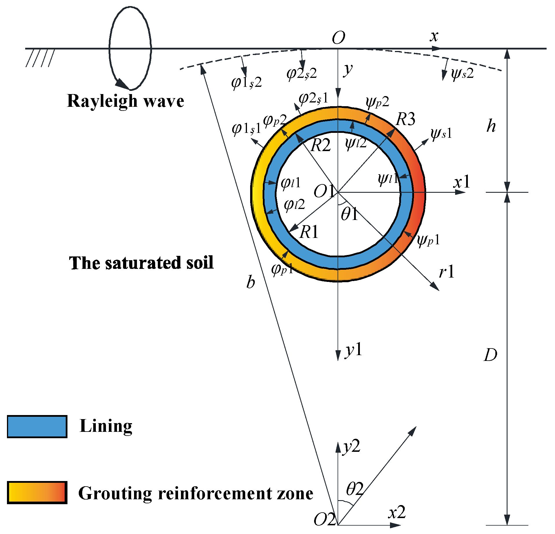
2. Theoretical Modeling

Figure 1 illustrates a multilayer cylindrical shallow tunnel embedded in a saturated isotropic soil medium at depth h. The grouting zone is modeled as a functionally graded interface between the tunnel lining and surrounding soil. The geometric configuration is defined by three radii: R₁ (lining inner radius), R₂ (lining outer radius), and R₃ (grouting reinforcement zone outer radius). The composite structure consists of an elastic, homogeneous, and isotropic lining-grouting system surrounded by saturated soil. To approximate the semi-infinite boundary condition, a large circular arc centered at O₂ with radius b = 1000R₁ is employed [32]. Coordinate transformations are facilitated through two polar coordinate systems: (r₁, θ₁) centered at O₁ (tunnel axis) and (r₂, θ₂) centered at O₂ (surface arc center). The ground surface aligns with the Cartesian coordinate origin (x, y), where the relationships between Cartesian and cylindrical coordinates are governed by the following transformations:

$$\mathrm{x}={\mathrm{x}}_1={\mathrm{x}}_2, \mathrm{y}=\mathrm{h}+{\mathrm{y}}_1, {\mathrm{r}}_1={\left({\mathrm{x}}_{1 }^2+{ \mathrm{y}}_1^2\right)}^{1/2}, {\mathsf{\theta }}_1=\arctan \left({\mathrm{x}}_1/{\mathrm{y}}_1\right), \mathrm{D}=\mathrm{b}-\mathrm{h}$$

(1)

2.1. Biot Theory of Poroelastic Medium

In geotechnical earthquake engineering applications, the applicability of Biot theory hinges on the soil’s grain size distribution, which governs pore geometry and hydraulic conductivity. Soils comprise assemblages of solid particles with varying sizes, where the effective pore diameter can be approximated as one-fifth of D₁₀, with D₁₀ denoting the grain diameter corresponding to 10% finer by weight in the particle size distribution curve [34]. Permeability (k_f), a critical parameter dictating pore fluid mobility, determines the validity of Biot’s poroelastic framework. Soils with k_f < 10⁻³ mm/s (e.g., fine silts and clays) are classified as poorly drained or impervious [35], where relative fluid–solid motion becomes negligible, rendering Biot’s wave equations inapplicable due to dominant quasi-static pore pressure diffusion.

Biot theory remains valid for soils with D₁₀ ranging from 0.05 mm to 1 mm, corresponding to permeability values conducive to dynamic fluid–solid interactions. This range encompasses fine to medium sands and certain silts, where interconnected pores facilitate measurable wave-induced fluid flow. Notably, soils within this D₁₀ spectrum exhibit sufficient permeability (k_f ≥ 10⁻³ mm/s) to sustain inertial coupling between the solid matrix and pore fluid under seismic frequencies, a prerequisite for Biot theory. However, heterogeneity in grain size distributions (e.g., gap-graded or well-graded sands) may necessitate site-specific calibration to account for variations in pore connectivity and tortuosity. Therefore, saturated soils that consist of fine to medium sands may be described by Biot theory [36].

According to the classic Biot theory, the governing equation for fluid-saturated soil in porous media can be obtained as

$$\begin{gathered} \mathrm{N}{\nabla }^2\mathbf{u}+\nabla \left[\left(\mathrm{A}+\mathrm{N}\right)\mathrm{e}+\mathrm{Q}\mathsf{\epsilon }\right]={\displaystyle \frac{{\partial }^2}{\partial {\mathrm{t}}^2}}\left({\mathsf{\rho }}_{11}\mathbf{u}+{\mathsf{\rho }}_{12}\mathbf{U}\right)+\widehat{\mathrm{b}}{\displaystyle \frac{\partial }{\partial \mathrm{t}}}\left(\mathbf{u}-\mathbf{U}\right) \\ \nabla \left[\mathrm{Qe}+\mathrm{R}\mathsf{\epsilon }\right]={\displaystyle \frac{{\partial }^2}{\partial {\mathrm{t}}^2}}\left({\mathsf{\rho }}_{12}\mathbf{u}+{\mathsf{\rho }}_{22}\mathbf{U}\right)+\widehat{\mathrm{b}}{\displaystyle \frac{\partial }{\partial \mathrm{t}}}\left(\mathbf{u}-\mathbf{U}\right) \end{gathered}$$

(2)

where $\mathbf{u}$ and $\mathbf{U}$ are the displacement of soil skeleton and the displacement of pore fluid, respectively; ${\nabla }^2$ is the Laplace operator; The symbols e and ε denote the bulk strains of the solid skeleton and pore fluid, respectively; $\mathrm{N},\mathrm{A},\mathrm{Q}$, and $\mathrm{R}$ are the elasticity constants of the saturated soil, $\mathrm{N}={\mathsf{\mu }}_{\mathrm{s}}=3{\mathrm{K}}_{\mathrm{b}}\left(1-2\mathrm{v}\right)/2\left(1+\mathrm{v}\right)$, $\mathrm{A}=\left({\mathrm{K}}_{\mathrm{b}}-2/3{\mathsf{\mu }}_{\mathrm{s}}\right)+{\mathrm{Q}}^2/\mathrm{R}, \mathrm{Q}=\mathrm{n}{\mathrm{K}}_{\mathrm{s}}^2\left(1-\mathrm{n}-{\mathrm{K}}_{\mathrm{b}}/{\mathrm{K}}_{\mathrm{s}}\right)/\left({\mathrm{K}}_{\mathrm{d}}-{\mathrm{K}}_{\mathrm{b}}\right), \mathrm{R}={\mathrm{n}}^2{\mathrm{K}}_{\mathrm{s}}^2/\left({\mathrm{K}}_{\mathrm{d}}-{\mathrm{K}}_{\mathrm{b}}\right), {\mathrm{K}}_{\mathrm{d}}={\mathrm{K}}_{\mathrm{s}}\left[1+\mathrm{n}\left({\mathrm{K}}_{\mathrm{s}}/{\mathrm{K}}_{\mathrm{f}}-1\right)\right],$ ${\mathrm{K}}_{\mathrm{b}}={\mathrm{K}}_{\mathrm{cr}}+\left(1-\mathrm{n}/{\mathrm{n}}_{\mathrm{cr}}\right)\left({\mathrm{K}}_{\mathrm{s}}-{\mathrm{K}}_{\mathrm{cr}}\right);$ ν denotes the Poisson’s ratio of the saturated soil matrix; Kₛ and K_b represent the bulk moduli of solid grains and the dry skeletal framework, respectively, with K_cr indicating the critical bulk modulus for framework collapse. The fluid phase is characterized by K_f (fluid bulk modulus) and η_f (fluid viscosity coefficient). Porosity-dependent parameters include n (saturated soil porosity) and n_cr (critical porosity threshold). Hydraulic transport properties are quantified through k_f (fluid permeability) and the dissipation coefficient $\widehat{\mathrm{b}}$ = (nₛη_f)/k_f, governing interstitial fluid–solid phase interactions. Here,

$$\begin{gathered} {\mathsf{\rho }}_{11}=\left(1 - {\mathrm{n}}_{\mathrm{s}}\right){\mathsf{\rho }}_{\mathrm{s}}+\mathsf{\gamma }\left(1-{ \mathrm{n}}_{\mathrm{s}}\right){\mathsf{\rho }}_{\mathrm{f}},{ \mathsf{\rho }}_{12}= \\ \hspace{1em}\hspace{1em}\hspace{1em}\hspace{1em}\hspace{1em}\hspace{1em}\hspace{1em}\hspace{1em}\hspace{1em}\hspace{1em}\hspace{1em}\hspace{1em}\hspace{1em}\hspace{1em}\hspace{1em} -\mathsf{\gamma }\left(1-{ \mathrm{n}}_{\mathrm{s}}\right){\mathsf{\rho }}_{\mathrm{f}},{ \mathsf{\rho }}_{22}={\mathrm{n}}_{\mathrm{s}}{\mathsf{\rho }}_{\mathrm{f}}+\mathsf{\gamma }\left(1-{ \mathrm{n}}_{\mathrm{s}}\right){\mathsf{\rho }}_{\mathrm{f}} \end{gathered}$$

(3)

where ${\mathsf{\rho }}_{\mathrm{s}}$ and ${\mathsf{\rho }}_{\mathrm{f}}$ represent the mass densities of the soil matrix and pore fluid, respectively. The inertial coupling coefficient γ, quantifying momentum transfer between phases, depends on the morphological characteristics of soil particles, with γ conventionally assigned value of 0.5 for spherical particulates.

The assumptions [12,13] for these wave equations are: (1) The soil skeleton is an ideal elastic, homogeneous, and isotropic porous medium obeying the generalized Hooke’s law, (2) elastic wavelengths significantly exceed the scale of pore heterogeneity, (3) pore fluid flow adheres to Darcy’s law, (4) The medium is statistically homogeneous and isotropic, with fully interconnected pores, and (5) Thermal effects are neglected. Assumptions (1) and (2) ensure the validity of continuum mechanics principles at the macroscopic scale. While porous media inherently exhibit solid–fluid discontinuities, deviations arise when incident wavelengths are sufficiently short to resolve individual pores, triggering microscale wave diffraction effects.

2.2. Potential Function of Governing Equation

Following the poroelastic wave propagation framework for porous fluid-saturated media, the governing wave equations are derived through Helmholtz decomposition of displacement fields. The solution methodology for Equation (2) employs scalar-vector potential formalism, where ϕ and ψ denote the dilatational and rotational potentials of the solid matrix, while Φ and Ψ represent analogous fluid phase potentials governing compressional and shear wave modes, shown as

$$\mathbf{u}=\nabla \mathsf{\varphi }+\nabla \times \mathbf{\psi }, \mathbf{U}=\nabla \mathsf{\Phi }+\nabla \times \mathbf{\Psi }$$

(4)

Substitution of Equation (4) into Equation (2), the following equations with potential functions can be presented as:

$$\left.\begin{array}{c}\left(\mathrm{A}+2\mathrm{N}\right){\nabla }^2\mathsf{\varphi }+\mathrm{Q}{\nabla }^2\mathsf{\Phi }={ \mathsf{\rho }}_{11}{\displaystyle \frac{{\partial }^2\mathsf{\varphi }}{\partial {\mathrm{t}}^2}}+{\mathsf{\rho }}_{12}{\displaystyle \frac{{\partial }^2\mathsf{\Phi }}{\partial {\mathrm{t}}^2}}+\widehat{\mathrm{b}}{\displaystyle \frac{\partial }{\partial \mathrm{t}}}\left(\mathsf{\varphi } - \mathsf{\Phi }\right) \\ \mathrm{Q}{\nabla }^2\mathsf{\varphi }+\mathrm{R}{\nabla }^2\mathsf{\Phi }={\mathsf{\rho }}_{12}{\displaystyle \frac{{\partial }^2\mathsf{\varphi }}{\partial {\mathrm{t}}^2}}+{\mathsf{\rho }}_{22}{\displaystyle \frac{{\partial }^2\mathsf{\Phi }}{\partial {\mathrm{t}}^2}}-\widehat{\mathrm{b}}{\displaystyle \frac{\partial }{\partial \mathrm{t}}}\left(\mathsf{\varphi } - \mathsf{\Phi }\right) \end{array}\right\}$$

(5)

$$\left.\begin{array}{c}\mathrm{N}{\nabla }^2\mathbf{\psi }={\mathsf{\rho }}_{11}{\displaystyle \frac{{\partial }^2\mathbf{\psi }}{\partial {\mathrm{t}}^2}}+{\mathsf{\rho }}_{12}{\displaystyle \frac{{\partial }^2\mathbf{\Psi }}{\partial {\mathrm{t}}^2}}+\widehat{ \mathrm{b}}{\displaystyle \frac{\partial }{\partial \mathrm{t}}}\left(\mathbf{\psi } - \mathbf{\Psi }\right)\\ 0={\mathsf{\rho }}_{12}{\displaystyle \frac{{\partial }^2\mathbf{\psi }}{\partial {\mathrm{t}}^2}}+{\mathsf{\rho }}_{22}{\displaystyle \frac{{\partial }^2\mathbf{\Psi }}{\partial {\mathrm{t}}^2}}-\widehat{\mathrm{b}}{\displaystyle \frac{\partial }{\partial \mathrm{t}}}\left(\mathbf{\psi } - \mathbf{\Psi }\right)\end{array}\right\}$$

(6)

where $\mathsf{\varphi }$ and Φ correspond to the compressional (P-wave) scalar potentials in the soil skeleton and pore fluid phases, respectively, characterizing volumetric deformation modes. Similarly, ψ and Ψ represent the shear-vertical (SV-wave) vector potentials describing distortional wavefields in the solid matrix and fluid phase, respectively, with directional particle motion perpendicular to the wavefront normal.

This study derives steady-state solutions for elastic wave scattering in the frequency domain. To isolate scattering effects from energy dissipation, assume the pore fluid viscosity is neglected (i.e., set to zero) and ${\mathsf{\eta }}_{\mathrm{f}}=0,\widehat{\mathrm{b}}=0$. For harmonic excitation, the time-explicit potential functions can be defined as:

$$\mathsf{\varphi }=\mathsf{\varphi }\left(\mathrm{x}, \mathrm{y}, \mathrm{z}\right){\mathrm{e}}^{-\mathrm{i}\mathsf{\omega }\mathrm{t}}, \mathsf{\Phi }=\mathsf{\Phi }\left(\mathrm{x}, \mathrm{y}, \mathrm{z}\right){\mathrm{e}}^{-\mathrm{i}\mathsf{\omega }\mathrm{t}}$$

(7)

$$\mathbf{\psi }=\mathbf{\psi }\left(\mathrm{x}, \mathrm{y}, \mathrm{z}\right){\mathrm{e}}^{-\mathrm{i}\mathsf{\omega }\mathrm{t}}, \mathbf{\Psi }=\mathbf{\Psi }\left(\mathrm{x}, \mathrm{y}, \mathrm{z}\right){\mathrm{e}}^{-\mathrm{i}\mathsf{\omega }\mathrm{t}}$$

(8)

where $\mathrm{i}=\sqrt{-1},\mathrm{t}$ is the time variable, $\mathsf{\omega }$ is the circular frequency. Substitution of Equations (7) and (8) into Equations (5) and (6) to eliminate $\mathsf{\Phi }$ and $\mathbf{\Psi }$, the equation in term of $\mathsf{\Phi }$ and $\mathbf{\Psi }$ can be obtained as

$$\left\{\begin{array}{l}\left({\nabla }^2+{\mathrm{k}}_{\mathsf{\alpha }1}^2\right){\mathsf{\varphi }}_1\\ \left({\nabla }^2+{\mathrm{k}}_{\mathsf{\alpha }2}^2\right){\mathsf{\varphi }}_2\\ \left({\nabla }^{2 }+{\mathrm{k}}_{\mathsf{\beta }}^2\right)\mathbf{\psi }\end{array}\right.$$

(9)

where the compressional wave potentials ϕ₁ (P₁) and ϕ₂ (P2) in the bulk material satisfy the superposition relation ϕ = ϕ₁ + ϕ₂, while the shear-vertical (SV) wave dynamics are characterized by the rotational potential ψ. ${\mathrm{k}}_{\mathsf{\alpha }1},{\mathrm{k}}_{\mathsf{\alpha }2}$ and ${\mathrm{k}}_{\mathsf{\beta }}$ are the wave numbers of P1 wave, P2 wave and SV wave in saturated soil, respectively, satisfying ${\mathrm{k}}_{\mathsf{\alpha }\mathrm{j}}={\displaystyle \frac{\mathsf{\omega }}{{\mathrm{c}}_{\mathsf{\alpha }\mathrm{j}}}} \left(\mathrm{j}=1, 2\right);{\mathrm{k}}_{\mathsf{\beta }}={\displaystyle \frac{\mathsf{\omega }}{{\mathrm{c}}_{\mathsf{\beta }}}},{\mathrm{c}}_{\mathsf{\alpha }\mathrm{j}} \left(\mathrm{j}=1, 2\right)$ are the wave velocities of P1 wave and P2 wave in saturated soil and ${\mathrm{c}}_{\mathsf{\beta }}$ is the SV wave velocity. Here,

$${\mathrm{c}}_{\mathsf{\alpha }\mathrm{j}}=\sqrt{{\displaystyle \frac{2\mathrm{B}}{\mathrm{C} \mp {\left({\mathrm{C}}^2-4\mathrm{BD}\right)}^{1/2}}}} \left(\mathrm{j}=1, 2\right);{ \mathrm{c}}_{\mathsf{\beta }}=\sqrt{{\displaystyle \frac{\mathrm{N}{\mathsf{\rho }}_{22}}{\mathrm{D}}}}$$

(10)

where $\mathrm{B}=\left(\mathrm{A}+2\mathrm{N}\right)\mathrm{R}-{\mathrm{Q}}^2,\mathrm{C}={\mathsf{\rho }}_{11}\mathrm{R}+{\mathsf{\rho }}_{22}\left(\mathrm{A}+2\mathrm{N}\right)-2{\mathsf{\rho }}_{12}\mathrm{Q}, \mathrm{D}={\mathsf{\rho }}_{11}{\mathsf{\rho }}_{22}-{\mathsf{\rho }}_{12}^2$. It can be derived from Equations (9) and (10) that there are three kinds of elastic body waves propagating in saturated soil, namely the P1 wave, P2 wave, and SV wave.

2.3. Incident Wave Field

This investigation examines the dynamic response of shallow-buried tunnel structures subjected to plane-strain Rayleigh wave fields propagating along the free surface of a saturated porous half-space. Unlike conventional scenarios involving P-wave or SV-wave incidence in saturated media—where impedance mismatches typically induce reflected waves at the free surface—Rayleigh wave excitation inherently satisfies traction-free boundary conditions through its elliptically polarized displacement field, thereby eliminating surface reflections as theoretically established in [37]. As depicted in Figure 1, the incident Rayleigh wave propagates along the x-axis with angular frequency ω, its displacement potential formalism following the analytical framework in [11].

$$\left\{\begin{array}{l}{\mathsf{\varphi }}_1^{\mathrm{R}}\left(\mathrm{x}, \mathrm{y}\right)={ \mathrm{A}}_1{\mathrm{e}}^{\left(\mathrm{i}{\mathrm{k}}_{\mathrm{R}}\mathrm{x}-{ \mathrm{v}}_{\mathsf{\alpha }1}\mathrm{y}\right)}{\mathrm{e}}^{-\mathrm{i}\mathsf{\omega }\mathrm{t}}\\ {\mathsf{\varphi }}_2^{\mathrm{R}}\left(\mathrm{x}, \mathrm{y}\right)={\mathrm{A}}_2{\mathrm{e}}^{\left(\mathrm{i}{\mathrm{k}}_{\mathrm{R}}\mathrm{x}-{ \mathrm{v}}_{\mathsf{\alpha }2}\mathrm{y}\right)}{\mathrm{e}}^{-\mathrm{i}\mathsf{\omega }\mathrm{t}}\\ {\mathbf{\psi }}^{\mathrm{R}}\left(\mathrm{x}, \mathrm{y}\right)=\mathrm{B}{\mathrm{e}}^{\left(\mathrm{i}{\mathrm{k}}_{\mathrm{R}}\mathrm{x} - {\mathrm{v}}_{\mathsf{\beta }}\mathrm{y}\right)}{\mathrm{e}}^{-\mathrm{i}\mathsf{\omega }\mathrm{t}}\end{array}\right.$$

(11)

where A₁, A₂ and B are the amplitudes of potential functions of Rayleigh waves; the superscript (R) denotes incident Rayleigh wave fields, where all wave potential functions inherently incorporate the time-harmonic factor e^($-$iωt). Following standard convention for harmonic analysis, this temporal component is subsequently omitted in the formulations hereinafter; k_R is the wave number of Rayleigh wave, satisfying

$$\begin{gathered} {\mathrm{v}}_{\mathsf{\alpha }1}=\sqrt{{\mathrm{k}}_{\mathrm{R}}^2 - {\mathrm{k}}_{\mathsf{\alpha }1}^2 }={\mathrm{k}}_{\mathrm{R}}\sqrt{1 - {\mathsf{\xi }}_1^2}, \\ {\mathrm{v}}_{\mathsf{\alpha }2}=\sqrt{{\mathrm{k}}_{\mathrm{R}}^2-{ \mathrm{k}}_{\mathsf{\alpha }2}^2}={\mathrm{k}}_{\mathrm{R}}\sqrt{1 - {\mathsf{\xi }}_2^2}, \\ { \mathrm{v}}_{\mathsf{\beta }}=\sqrt{{\mathrm{k}}_{\mathrm{R}}^2-{\mathrm{k}}_{\mathsf{\beta } }^2}={ \mathrm{k}}_{\mathrm{R}}\sqrt{1 - \mathsf{\xi }} \end{gathered}$$

where ${\mathsf{\xi }}^2={ \left({\mathrm{c}}_{\mathrm{R}}/{\mathrm{c}}_{\mathsf{\beta }}\right)}^2$, ${\mathsf{\xi }}_1^2={ \left({\mathrm{c}}_{\mathrm{R}}/{\mathrm{c}}_{\mathsf{\alpha }1}\right)}^2={\mathrm{c}}_1{\mathsf{\xi }}^2$, ${\mathsf{\xi }}_2^2={\left({\mathrm{c}}_{\mathrm{R}}/{\mathrm{c}}_{\mathsf{\alpha }2}\right)}^2={\mathrm{c}}_2{\mathsf{\xi }}^2$, ${\mathrm{c}}_1={\left({\mathrm{c}}_{\mathsf{\beta }}/{\mathrm{c}}_{\mathsf{\alpha }1}\right)}^2={\mathrm{c}}_1{\mathsf{\xi }}^2$, ${\mathrm{c}}_2={\left({\mathrm{c}}_{\mathsf{\beta }}/{\mathrm{c}}_{\mathsf{\alpha }2}\right)}^2={\mathrm{c}}_2{\mathsf{\xi }}^2$; ${\mathrm{c}}_{\mathrm{R}}$ is the wave velocity of $\mathrm{R}$ wave.

The wave functions in Equation (11) can be expressed in cylindrical coordinate $\left({\mathrm{r}}_1,{\mathsf{\theta }}_1\right),$ as follows:

$$\left\{\begin{array}{l}{\mathsf{\varphi }}_1^{\mathrm{R}}\left({\mathrm{r}}_{1 }, {\mathsf{\theta }}_1\right)={\mathrm{A}}_1{\mathrm{e}}^{\left(\mathrm{i}{\mathrm{k}}_{\mathrm{R}}{\mathrm{r}}_1\sin {\mathsf{\theta }}_{1 }-{ \mathrm{v}}_{\mathsf{\alpha }1}{\mathrm{r}}_1\cos {\mathsf{\theta }}_1-{\mathrm{v}}_{\mathsf{\alpha }1}\mathrm{h}\right)}\\ {\mathsf{\varphi }}_2^{\mathrm{R}}\left({\mathrm{r}}_1, {\mathsf{\theta }}_1\right)={ \mathrm{A}}_2{\mathrm{e}}^{\left(\mathrm{i}{\mathrm{k}}_{\mathrm{R}}{\mathrm{r}}_1\sin {\mathsf{\theta }}_1-{\mathrm{v}}_{\mathsf{\alpha }2}{\mathrm{r}}_1\cos {\mathsf{\theta }}_{1 }-{ \mathrm{v}}_{\mathsf{\alpha }2}\mathrm{h}\right)}\\ {\mathbf{\psi }}^{\mathrm{R}}\left({\mathrm{r}}_{1 }, {\mathsf{\theta }}_1\right)=\mathrm{B}{\mathrm{e}}^{\left(\mathrm{i}{\mathrm{k}}_{\mathrm{R}}{\mathrm{r}}_1\sin {\mathsf{\theta }}_{1 }-{ \mathrm{v}}_{\mathsf{\beta }}{\mathrm{r}}_1\cos {\mathsf{\theta }}_{1 }-{ \mathrm{v}}_{\mathsf{\beta }}\mathrm{h}\right)}\end{array}\right.$$

(12)

where the amplitudes ${\mathrm{A}}_1,{ \mathrm{A}}_2$ and $\mathrm{B}$ can be obtained using zero stress boundary condition of half space ground surface [11], presented as

$$\left[\begin{array}{ccc}2-{\mathrm{M}}_1{\mathsf{\xi }}_1^2& 2-{\mathrm{M}}_2{\mathsf{\xi }}_2^2& -2\mathrm{i}\sqrt{1-{\mathsf{\xi }}^2}\\ 2\mathrm{i}\sqrt{1-{\mathsf{\xi }}_1^2}& 2\mathrm{i}\sqrt{1-{\mathsf{\xi }}_2^2}& 2-{\mathsf{\xi }}^2\\ -{\mathrm{S}}_1{\mathsf{\xi }}_1^2& -{\mathrm{S}}_2{\mathsf{\xi }}_2^2& 0\end{array}\right]\left[\begin{array}{l}{\mathrm{A}}_1\\ {\mathrm{A}}_2\\ \mathrm{B}\end{array}\right]=\left\{\begin{array}{l}0\\ 0\\ 0\end{array}\right\}$$

(13)

where ${\mathrm{M}}_{\mathrm{j}}=\left(\mathrm{A}+2\mathrm{N}+{\mathsf{\eta }}_{\mathrm{j}}\mathrm{Q}\right)/{\mathsf{\mu }}_{\mathrm{s}}\left(\mathrm{j}=1,2\right);{\mathrm{S}}_{\mathrm{j}}=\left(\mathrm{Q}+{\mathsf{\eta }}_{\mathrm{j}}\mathrm{R}\right)/{\mathsf{\mu }}_{\mathrm{s}}\left(\mathrm{j}=1,2\right)$.

The existence of nontrivial solutions for the system governed by Equation (13) is contingent upon the zero value of its determinant. Then, the wave velocity equation of R wave in saturated half space under surface pervious boundary condition can be obtained as

$${\left(2-{\mathsf{\xi }}^2\right)}^2-4\sqrt{1-{\mathsf{\xi }}^2}\left({\mathsf{\kappa }}_2\sqrt{1-{\mathrm{c}}_1{\mathsf{\xi }}^2}-{\mathsf{\kappa }}_1\sqrt{1-{\mathrm{c}}_2{\mathsf{\xi }}^2}\right)=0$$

(14)

where ${\mathsf{\kappa }}_{\mathrm{j}}={\mathrm{c}}_{\mathrm{j}}{\mathrm{S}}_{\mathrm{j}}/\left({\mathrm{c}}_2{\mathrm{S}}_2-{\mathrm{c}}_1{\mathrm{S}}_1\right)\left(\mathrm{j}=1, 2\right)$.

Equation (14) governs the propagation of Rayleigh waves in a fluid-saturated poroelastic half-space, demonstrating frequency-independent phase velocity (i.e., non-dispersive behavior) under inviscid fluid conditions. The amplitude coefficients of Rayleigh wave potentials are uniquely quantified upon solving for the characteristic parameter ξ from Equation (14). Notably, the existence of real or complex roots for this dispersion equation depends critically on the material constitutive properties, reflecting distinct wave attenuation regimes in heterogeneous medium.

By using the Rayleigh wave velocity equation, ${\mathsf{\xi }}^2$ can be obtained, and then ${\mathrm{k}}_{\mathrm{R}},{\mathrm{v}}_{\mathsf{\alpha }1},{\mathrm{v}}_{\mathsf{\alpha }2},{\mathrm{v}}_{\mathsf{\beta }}$ can be obtained, further solving for the coefficients of the incident Rayleigh wave potential function ${\mathrm{A}}_1,{\mathrm{A}}_2,\mathrm{B}$.

2.4. Scattering Wave Field in Soil

The interaction between incident Rayleigh waves and the tunnel’s grouted reinforcement boundary initiates radiative scattering within the saturated soil matrix. By constraining these scattered waves to satisfy the orthogonality condition prescribed by the wave eigenfunctions in Equation (9), their general solution admits the following multipole expansion:

$$\left\{\begin{array}{l}{\mathsf{\varphi }}_{1,\mathrm{s}1}\left({\mathrm{r}}_1,{\mathsf{\theta }}_1\right)={\displaystyle \sum _{\mathrm{n}=0}^{\infty }}{\mathrm{H}}_{\mathrm{n}}^{\left(1\right)}\left({\mathrm{k}}_{\mathrm{s}\mathsf{\alpha },1} {\mathrm{r}}_1\right)\left({\mathrm{A}}_{\mathrm{s}1,\mathrm{n}}^{\left(1\right)}\cos \mathrm{n}{\mathsf{\theta }}_1+{\mathrm{B}}_{\mathrm{s}1,\mathrm{n}}^{\left(1\right)}\sin \mathrm{n}{\mathsf{\theta }}_1\right)\\ {\mathsf{\varphi }}_{2,\mathrm{s}1}\left({\mathrm{r}}_1,{\mathsf{\theta }}_1\right)={\displaystyle \sum _{\mathrm{n}=0}^{\infty }}{\mathrm{H}}_{\mathrm{n}}^{\left(1\right)}\left({\mathrm{k}}_{\mathrm{s}\mathsf{\alpha },2} {\mathrm{r}}_1\right)\left({\mathrm{C}}_{\mathrm{s}1,\mathrm{n}}^{\left(1\right)}\cos \mathrm{n}{\mathsf{\theta }}_1+{\mathrm{D}}_{\mathrm{s}1,\mathrm{n}}^{\left(1\right)}\sin \mathrm{n}{\mathsf{\theta }}_1\right)\\ {\mathbf{\psi }}_{\mathrm{s}1}\left({\mathrm{r}}_1,{\mathsf{\theta }}_1\right)={\displaystyle \sum _{\mathrm{n}=0}^{\infty }}{\mathrm{H}}_{\mathrm{n}}^{\left(1\right)}\left({\mathrm{k}}_{\mathrm{s}\mathsf{\beta }} {\mathrm{r}}_1\right)\left({\mathrm{E}}_{\mathrm{s}1,\mathrm{n}}^{\left(1\right)}\sin \mathrm{n}{\mathsf{\theta }}_{1 }+{\mathrm{F}}_{\mathrm{s}1,\mathrm{n}}^{\left(1\right)}\cos \mathrm{n}{\mathsf{\theta }}_1\right)\end{array}\right.$$

(15)

where the scattered wave fields in the polar coordinate system (r₁, θ₁) are governed by the potential functions ϕ_1,s1 (fast P₁-wave), ϕ_2,s1 (slow P₂-wave), and ψ_s1 (SV-wave), expressed through cylindrical harmonic expansions. These solutions employ first-kind Hankel functions ${\mathrm{H}}_{\mathrm{n}}^{\left(1\right)}\left(\cdot \right)$ of order n, where the amplitude coefficients ${\mathrm{A}}_{\mathrm{s}1,\mathrm{n}}^{\left(1\right)},{\mathrm{B}}_{\mathrm{s}1,\mathrm{n}}^{\left(1\right)},{\mathrm{C}}_{\mathrm{s}1,\mathrm{n}}^{\left(1\right)},{\mathrm{D}}_{\mathrm{s}1,\mathrm{n}}^{\left(1\right)},{\mathrm{E}}_{\mathrm{s}1,\mathrm{n}}^{\left(1\right)}$ and ${\mathrm{F}}_{\mathrm{s}1,\mathrm{n}}^{\left(1\right)}$ represent undetermined multipole expansion constants to be resolved through boundary matching conditions.

Furthermore, an additional kind of convergent scattering waves which are corresponding to potential functions ${\mathsf{\varphi }}_{1,\mathrm{s}2}, {\mathsf{\varphi }}_{2,\mathrm{s}2}$ and ${\mathbf{\psi }}_{\mathrm{s}2}$, generate for the reflection of the scattering waves of ${\mathrm{P}}_1,{\mathrm{P}}_2$ and SV above by the ground surface under the assumption of large circular arch simplification. The potential functions of these scattering waves similarly can be expressed as

$$\left\{\begin{array}{l}{\mathsf{\varphi }}_{1,\mathrm{s}2}\left({\mathrm{r}}_2, {\mathsf{\theta }}_2\right)={\displaystyle \sum _{\mathrm{m}=0}^{\infty }}{\mathrm{J}}_{\mathrm{m}}^{\left(1\right)}\left({\mathrm{k}}_{\mathrm{s}\mathsf{\alpha },1} {\mathrm{r}}_2\right)\left({\mathrm{A}}_{\mathrm{s}2, \mathrm{m}}^{\left(2\right)}\cos \mathrm{m}{\mathsf{\theta }}_2+{\mathrm{B}}_{\mathrm{s}2, \mathrm{m}}^{\left(2\right)}\sin \mathrm{m}{\mathsf{\theta }}_2\right)\\ {\mathsf{\varphi }}_{2,\mathrm{s}2}\left({\mathrm{r}}_2, {\mathsf{\theta }}_2\right)={\displaystyle \sum _{\mathrm{m}=0}^{\infty }}{\mathrm{J}}_{\mathrm{m}}^{\left(1\right)}\left({\mathrm{k}}_{\mathrm{s}\mathsf{\alpha },2} {\mathrm{r}}_2\right)\left({\mathrm{C}}_{\mathrm{s}2, \mathrm{m}}^{\left(2\right)}\cos \mathrm{m}{\mathsf{\theta }}_2+{\mathrm{D}}_{\mathrm{s}2, \mathrm{m}}^{\left(2\right)}\sin \mathrm{m}{\mathsf{\theta }}_2\right)\\ {\mathbf{\psi }}_{\mathrm{s}2}\left({\mathrm{r}}_2,{ \mathsf{\theta }}_2\right)={\displaystyle \sum _{\mathrm{m}=0}^{\infty }}{\mathrm{J}}_{\mathrm{m}}^{\left(1\right)}\left({\mathrm{k}}_{\mathrm{s}\mathsf{\beta }}{\mathrm{r}}_2\right)\left({\mathrm{E}}_{\mathrm{s}2, \mathrm{m}}^{\left(2\right)}\sin \mathrm{m}{\mathsf{\theta }}_2+{\mathrm{F}}_{\mathrm{s}2, \mathrm{m}}^{\left(2\right)}\cos \mathrm{m}{\mathsf{\theta }}_2\right)\end{array}\right.$$

(16)

where ${\mathsf{\varphi }}_{1,\mathrm{s}2},{\mathsf{\varphi }}_{2,\mathrm{s}2}$ and ${\mathbf{\psi }}_{\mathrm{s}2}$ are in coordinate system $\left({\mathrm{r}}_2,{\mathsf{\theta }}_2\right);{\mathrm{J}}_{\mathrm{m}}^{\left(1\right)}\left(\cdot \right)$ is the first kind of n-order Bessel function; ${\mathrm{A}}_{\mathrm{s}2,\mathrm{m}}^{\left(2\right)},{\mathrm{B}}_{\mathrm{s}2,\mathrm{m}}^{\left(2\right)}$, ${\mathrm{C}}_{\mathrm{s}2,\mathrm{m}}^{\left(2\right)},{\mathrm{D}}_{\mathrm{s}2,\mathrm{m}}^{\left(2\right)},{\mathrm{E}}_{\mathrm{s}2,\mathrm{m}}^{\left(2\right)}\hspace{0.33em}$ and ${\mathrm{F}}_{\mathrm{s}2,\mathrm{m}}^{\left(2\right)}$ are the undetermined coefficients.

2.5. Total Wave Field Potential Function in Saturated Soil

The resultant wavefield within the solid phase of the saturated porous medium emerges from the superposition of the free-field incident Rayleigh wave and multiscale scattering mechanisms, incorporating surface-generated P1, P2, and SV waves at the soil-air interface, as well as interfacial scattering of analogous wave modes induced by impedance contrast at the soil-grouting reinforcement boundary. Through rigorous application of wavefield superposition principles, the total dynamic potential function governing solid-phase displacements—encompassing both primary wave propagation and secondary scattering phenomena—is analytically derived and formally expressed in Equation (17), establishing a unified framework for quantifying multipath wave interactions in heterogeneous poroelastic media.

$$\begin{gathered} \mathsf{\varphi }={ \mathsf{\varphi }}_1^{\mathrm{R}}+{\mathsf{\varphi }}_2^{\mathrm{R}}+{ \mathsf{\varphi }}_{1,\mathrm{s}1}+{ \mathsf{\varphi }}_{2,\mathrm{s}1}+{ \mathsf{\varphi }}_{1,\mathrm{s}2}+{ \mathsf{\varphi }}_{2,\mathrm{s}2} \\ \mathsf{\psi }={\mathsf{\psi }}^{\mathrm{R}}+{ \mathsf{\psi }}_{\mathrm{s}1}+{ \mathsf{\psi }}_{\mathrm{s}2} \end{gathered}$$

(17)

For determining the wave field potential function of the fluid phase, substitute Equation (7) into Equation (5) and obtain

$$\begin{gathered} \mathsf{\Phi }={ \mathsf{\eta } }_1\left({\mathsf{\varphi }}_1^{\mathrm{R}}+{\mathsf{\varphi }}_{1,\mathrm{s}1}+{\mathsf{\varphi }}_{1,\mathrm{s}2}\right)+{\mathsf{\eta }}_2\left({\mathsf{\varphi }}_2^{\mathrm{R}}+{ \mathsf{\varphi }}_{2,\mathrm{s}1}+{\mathsf{\varphi }}_{2,\mathrm{s}2}\right) \\ \mathbf{\Psi }={ \mathsf{\eta } }_3\left({\mathbf{\psi }}^{\mathrm{R}}+{\mathbf{\psi }}_{\mathrm{s}1}+{\mathbf{\psi }}_{\mathrm{s}2}\right) \end{gathered}$$

(18)

where

$$\begin{array}{c}{\mathsf{\eta }}_{\mathrm{j}}={\displaystyle \frac{\frac{\mathrm{B}}{{\mathrm{V}}_{\mathsf{\alpha },\mathrm{j}}^2}-{\mathsf{\rho }}_{11}\mathrm{R}+{\mathsf{\rho }}_{12}\mathrm{Q}}{{\mathsf{\rho }}_{12}\mathrm{R} - {\mathsf{\rho }}_{22}\mathrm{Q}}}, \left(\mathrm{j}=1,2\right)\hfill \\ {\mathsf{\eta }}_3=-{\displaystyle \frac{{\mathsf{\rho }}_{12}}{{\mathsf{\rho }}_{22}}}\hfill \end{array}$$

2.6. Scattered Field Wave Potential Function in the Grouting Reinforcement Zone

The grouting zone contains cohesive scattered P waves ${\mathsf{\varphi }}_{\mathrm{p}1}\left({\mathrm{r}}_1,{\mathsf{\theta }}_1\right)$ and SV waves ${\mathbf{\psi }}_{\mathrm{p}1}\left({\mathrm{r}}_1,{\mathsf{\theta }}_1\right)$ produced at the interface with the saturated soil, together with outgoing scattered P waves ${\mathsf{\varphi }}_{\mathrm{p}2}\left({\mathrm{r}}_1,{\mathsf{\theta }}_1\right)$ and SV waves ${\mathbf{\psi }}_{\mathrm{p}2}\left({\mathrm{r}}_1,{\mathsf{\theta }}_1\right)$ formed at the interface with the lining. The wave potential function in the grouting reinforcement layer is expressed as a Fourier–Bessel series.

$$\left\{\begin{array}{c}{\mathsf{\varphi }}_{\mathrm{p}1}\left({\mathrm{r}}_1,{\mathsf{\theta }}_1\right)={\displaystyle \sum _{\mathrm{m}=0}^{\infty }}{\mathrm{J}}_{\mathrm{n}}\left({\mathrm{k}}_{\mathrm{p}\mathsf{\alpha }}{\mathrm{r}}_1\right)\left({\mathrm{A}}_{\mathrm{p}1,\mathrm{n}}^{\left(1\right)}\cos \mathrm{n}{\mathsf{\theta }}_1+{\mathrm{B}}_{\mathrm{p}1,\mathrm{n}}^{\left(1\right)}\sin \mathrm{n}{\mathsf{\theta }}_1\right)\\ {\mathbf{\psi }}_{\mathrm{p}1}\left({\mathrm{r}}_1,{\mathsf{\theta }}_1\right)={\displaystyle \sum _{\mathrm{m}=0}^{\infty }}{\mathrm{J}}_{\mathrm{n}}\left({\mathrm{k}}_{\mathrm{p}\mathsf{\beta }}{\mathrm{r}}_1\right)\left({\mathrm{E}}_{\mathrm{p}1,\mathrm{n}}^{\left(1\right)}\sin \mathrm{n}{\mathsf{\theta }}_1+{\mathrm{F}}_{\mathrm{p}1,\mathrm{n}}^{\left(1\right)}\cos \mathrm{n}{\mathsf{\theta }}_1\right)\\ {\mathsf{\varphi }}_{\mathrm{p}2}\left({\mathrm{r}}_1,{\mathsf{\theta }}_1\right)={\displaystyle \sum _{\mathrm{m}=0}^{\infty }}{\mathrm{H}}_{\mathrm{n}}^{\left(1\right)}\left({\mathrm{k}}_{\mathrm{p}\mathsf{\alpha }}{\mathrm{r}}_1\right)\left({\mathrm{A}}_{\mathrm{p}2,\mathrm{n}}^{\left(1\right)}\cos \mathrm{n}{\mathsf{\theta }}_1+{ \mathrm{B}}_{\mathrm{p}2,\mathrm{n}}^{\left(1\right)}\sin \mathrm{n}{\mathsf{\theta }}_1\right)\\ {\mathbf{\psi }}_{\mathrm{p}2}\left({\mathrm{r}}_1,{\mathsf{\theta }}_1\right)={\displaystyle \sum _{\mathrm{m}=0}^{\infty }}{\mathrm{H}}_{\mathrm{n}}^{\left(1\right)}\left({\mathrm{k}}_{\mathrm{p}\mathsf{\beta }}{\mathrm{r}}_1\right)\left({\mathrm{E}}_{\mathrm{p}2,\mathrm{n}}^{\left(1\right)}\sin \mathrm{n}{\mathsf{\theta }}_{1 }+{\mathrm{F}}_{\mathrm{p}2,\mathrm{n}}^{\left(1\right)}\cos \mathrm{n}{\mathsf{\theta }}_1\right)\end{array}\right.$$

(19)

where ${\mathrm{k}}_{\mathrm{p}\mathsf{\alpha }}=\mathsf{\omega }/{\mathrm{c}}_{\mathrm{p},\mathrm{p}},{\mathrm{k}}_{\mathrm{p}\mathsf{\beta }}=\mathsf{\omega }/{\mathrm{c}}_{\mathrm{s},\mathrm{p}}$ represents the wave numbers of the $\mathrm{P}$ wave and $\mathrm{S}\mathrm{V}$ wave in the grouting reinforcement zone, and ${\mathrm{c}}_{\mathrm{p},\mathrm{p}},{\mathrm{c}}_{\mathrm{s},\mathrm{p}}$ represents the wave speeds of the $\mathrm{P}$ wave and $\mathrm{S}\mathrm{V}$ wave in the grouting reinforcement zone. ${\mathrm{A}}_{\mathrm{p}1,\mathrm{n}}^{\left(1\right)},{\mathrm{B}}_{\mathrm{p}1,\mathrm{n}}^{\left(1\right)},{\mathrm{E}}_{\mathrm{p}1,\mathrm{n}}^{\left(1\right)},{\mathrm{F}}_{\mathrm{p}1,\mathrm{n}}^{\left(1\right)},{\mathrm{A}}_{\mathrm{p}2,\mathrm{n}}^{\left(1\right)},{\mathrm{B}}_{\mathrm{p}2,\mathrm{n}}^{\left(1\right)},{\mathrm{E}}_{\mathrm{p}2,\mathrm{n}}^{\left(1\right)},$ ${\mathrm{F}}_{\mathrm{p}2,\mathrm{n}}^{\left(1\right)}$ are the undetermined coefficients. The expression for the total wave potential function in the grouting reinforcement zone can be obtained as

$$\left\{\begin{array}{c}{\mathsf{\varphi }}_{\mathrm{p}}={\mathsf{\varphi }}_{\mathrm{p}1}+{\mathsf{\varphi }}_{\mathrm{p}2}\\ {\mathbf{\psi }}_{\mathrm{p}}={\mathbf{\psi }}_{\mathrm{p}1 }+{ \mathbf{\psi }}_{\mathrm{p}2}\end{array}\right.$$

(20)

2.7. Scattered Field Wave Potential Function in the Tunnel Lining

In the tunnel lining, there are cohesive scattered $\mathrm{P}$ waves ${\mathsf{\varphi }}_{\mathrm{l}1}\left({\mathrm{r}}_1,{\mathsf{\theta }}_1\right)$ and $\mathrm{SV}$ waves ${\mathbf{\psi }}_{\mathrm{l}1}\left({\mathrm{r}}_1,{\mathsf{\theta }}_1\right)$ generated at the interface with the grouting zone, as well as outgoing scattered $\mathrm{P}$ waves ${\mathsf{\varphi }}_{\mathrm{l}2}\left({\mathrm{r}}_1,{\mathsf{\theta }}_1\right)$ and $\mathrm{SV}$ waves ${\mathbf{\psi }}_{\mathrm{l}2}\left({\mathrm{r}}_1,{\mathsf{\theta }}_1\right)$ generated at the free surface of the lining. The potential function in the lining is expanded in the form of a Fourier–Bessel series.

$$\left\{\begin{array}{c}{\mathsf{\varphi }}_{\mathrm{l}1}\left({\mathrm{r}}_1,{\mathsf{\theta }}_1\right)={\displaystyle \sum _{\mathrm{m}=0}^{\infty }}{\mathrm{J}}_{\mathrm{n}}\left({\mathrm{k}}_{\mathrm{l}\mathsf{\alpha }}{\mathrm{r}}_1\right)\left({\mathrm{A}}_{\mathrm{l}1,\mathrm{n}}^{\left(1\right)}\cos \mathrm{n}{\mathsf{\theta }}_1+{\mathrm{B}}_{\mathrm{l}1,\mathrm{n}}^{\left(1\right)}\sin \mathrm{n}{\mathsf{\theta }}_1\right)\\ {\mathbf{\psi }}_{\mathrm{l}1}\left({\mathrm{r}}_1,{\mathsf{\theta }}_1\right)={\displaystyle \sum _{\mathrm{m}=0}^{\infty }}{\mathrm{J}}_{\mathrm{n}}\left({\mathrm{k}}_{\mathrm{l}\mathsf{\beta }}{\mathrm{r}}_1\right)\left({\mathrm{E}}_{\mathrm{l}1,\mathrm{n}}^{\left(1\right)}\sin \mathrm{n}{\mathsf{\theta }}_1+{\mathrm{F}}_{\mathrm{l}1,\mathrm{n}}^{\left(1\right)}\cos \mathrm{n}{\mathsf{\theta }}_1\right)\\ {\mathsf{\varphi }}_{\mathrm{l}2}\left({\mathrm{r}}_1,{\mathsf{\theta }}_1\right)={\displaystyle \sum _{\mathrm{m}=0}^{\infty }}{\mathrm{H}}_{\mathrm{n}}^{\left(1\right)}\left({\mathrm{k}}_{\mathrm{l}\mathsf{\alpha }}{\mathrm{r}}_1\right)\left({\mathrm{A}}_{\mathrm{l}2,\mathrm{n}}^{\left(1\right)}\cos \mathrm{n}{\mathsf{\theta }}_1+{\mathrm{B}}_{\mathrm{l}2,\mathrm{n}}^{\left(1\right)}\sin \mathrm{n}{\mathsf{\theta }}_1\right)\\ {\mathbf{\psi }}_{\mathrm{l}2}\left({\mathrm{r}}_1,{\mathsf{\theta }}_1\right)={\displaystyle \sum _{\mathrm{m}=0}^{\infty }}{\mathrm{H}}_{\mathrm{n}}^{\left(1\right)}\left({\mathrm{k}}_{\mathrm{l}\mathsf{\beta }}{\mathrm{r}}_1\right)\left({\mathrm{E}}_{\mathrm{l}2,\mathrm{n}}^{\left(1\right)}\sin \mathrm{n}{\mathsf{\theta }}_1+{\mathrm{F}}_{\mathrm{l}2,\mathrm{n}}^{\left(1\right)}\cos \mathrm{n}{\mathsf{\theta }}_1\right)\end{array}\right.$$

(21)

where ${\mathrm{k}}_{\mathrm{l}\mathsf{\alpha }}=\mathsf{\omega }/{\mathrm{c}}_{\mathrm{p},\mathrm{l}},{\mathrm{k}}_{\mathrm{l}\mathsf{\beta }}=\mathsf{\omega }/{\mathrm{c}}_{\mathrm{s},\mathrm{l}}$ are the wavenumbers of the $\mathrm{P}$ wave and $\mathrm{SV}$ wave in the lining, respectively, and ${\mathrm{c}}_{\mathrm{p},\mathrm{l}},{\mathrm{c}}_{\mathrm{s},\mathrm{l}}$ are the wave velocities of the $\mathrm{P}$ wave and $\mathrm{S}\mathrm{V}$ wave in the lining, respectively. ${\mathrm{A}}_{\mathrm{l}1,\mathrm{n}}^{\left(1\right)},{\mathrm{B}}_{\mathrm{l}1,\mathrm{n}}^{\left(1\right)},{\mathrm{E}}_{\mathrm{l}1,\mathrm{n}}^{\left(1\right)},{\mathrm{F}}_{\mathrm{l}1,\mathrm{n}}^{\left(1\right)},{\mathrm{A}}_{\mathrm{l}2,\mathrm{n}}^{\left(1\right)},{\mathrm{B}}_{\mathrm{l}2,\mathrm{n}}^{\left(1\right)},{\mathrm{E}}_{\mathrm{l}2,\mathrm{n}}^{\left(1\right)},{\mathrm{F}}_{\mathrm{l}2,\mathrm{n}}^{\left(1\right)}$ is the undetermined coefficient. Then, the expression for the total wave potential function in the lining can be obtained as

$$\left\{\begin{array}{c}{\mathsf{\varphi }}_{\mathrm{l}}={\mathsf{\varphi }}_{\mathrm{l}1}+{\mathsf{\varphi }}_{\mathrm{l}2}\\ {\mathbf{\psi }}_{\mathrm{l}}={\mathbf{\psi }}_{\mathrm{l}1}+{\mathbf{\psi }}_{\mathrm{l}2}\end{array}\right.$$

(22)

3. Boundary Conditions and the Solutions

3.1. Boundary Conditions

To solve the values of the undetermined coefficients $\left\{{\mathrm{A}}_{\mathrm{s}1,\mathrm{n}}^{\left(1\right)},{\mathrm{B}}_{\mathrm{s}1,\mathrm{n}}^{\left(1\right)},{\mathrm{C}}_{\mathrm{s}1,\mathrm{n}}^{\left(1\right)},{\mathrm{D}}_{\mathrm{s}1,\mathrm{n}}^{\left(1\right)},{\mathrm{E}}_{\mathrm{s}1,\mathrm{n}}^{\left(1\right)},{\mathrm{F}}_{\mathrm{s}1,\mathrm{n}}^{\left(1\right)}\right\},$ $\left\{{\mathrm{A}}_{\mathrm{s}2,\mathrm{m}}^{\left(2\right)},{\mathrm{B}}_{\mathrm{s}2,\mathrm{m}}^{\left(2\right)},{\mathrm{C}}_{\mathrm{s}2,\mathrm{m}}^{\left(2\right)},{\mathrm{D}}_{\mathrm{s}2,\mathrm{m}}^{\left(2\right)},{\mathrm{E}}_{\mathrm{s}2,\mathrm{m}}^{\left(2\right)},{\mathrm{F}}_{\mathrm{s}2,\mathrm{m}}^{\left(2\right)}\right\}$, $\left\{{{\mathrm{A}}_{\mathrm{p}1,\mathrm{n}}^{\left(1\right)},\mathrm{B}}_{\mathrm{p}1,\mathrm{n}}^{\left(1\right)},{\mathrm{E}}_{\mathrm{p}1,\mathrm{n}}^{\left(1\right)},{\mathrm{F}}_{\mathrm{p}1,\mathrm{n}}^{\left(1\right)},{\mathrm{A}}_{\mathrm{p}2,\mathrm{n}}^{\left(1\right)},{\mathrm{B}}_{\mathrm{p}2,\mathrm{n}}^{\left(1\right)},{\mathrm{E}}_{\mathrm{p}2,\mathrm{n}}^{\left(1\right)},{\mathrm{F}}_{\mathrm{p}2,\mathrm{n}}^{\left(1\right)}\right\}$ and $\left.{\left\{{\mathrm{A}}_{\mathrm{l}1,\mathrm{n}}^{\left(1\right)}\right.,\mathrm{B}}_{\mathrm{l}1,\mathrm{n}}^{\left(1\right)},{\mathrm{E}}_{\mathrm{l}1,\mathrm{n}}^{\left(1\right)},{\mathrm{F}}_{\mathrm{l}1,\mathrm{n}}^{\left(1\right)},{\mathrm{A}}_{\mathrm{l}2,\mathrm{n}}^{\left(1\right)},{\mathrm{B}}_{\mathrm{l}2,\mathrm{n}}^{\left(1\right)},{\mathrm{E}}_{\mathrm{l}2,\mathrm{n}}^{\left(1\right)},{\mathrm{F}}_{\mathrm{l}2,\mathrm{n}}^{\left(1\right)}\right\}$, the boundary conditions at the interface need to be utilized. This paper assumes that the interface between the saturated soil and the lining is an impermeable boundary. In this paper the natural ground surface can be considered as permeable boundary conditions. Then the boundary conditions can be shown as

• Stress boundary condition at the surface of saturated soil;

  $$\left\{\begin{array}{c}{\mathsf{\tau }}_{\mathrm{rr}}^{\mathrm{S}}={\mathsf{\tau }}_{\mathrm{r}\mathsf{\theta }}^{\mathrm{S}}=0\\ \mathsf{\sigma }=0\end{array}\right.\mathrm{at} \mathrm{r}=\mathrm{b} \mathrm{in} \left({\mathrm{r}}_2,{\mathsf{\theta }}_2\right) \mathrm{system}$$

  (23)
• Displacement boundary condition at the interface between saturated soil and grouting reinforcement zone;

  $$\left\{\begin{array}{c}{\mathrm{u}}_{\mathrm{r}}^{\mathrm{S}}={\mathrm{u}}_{\mathrm{r}}^{\mathrm{p}}\\ {\mathrm{u}}_{\mathsf{\theta }}^{\mathrm{S}}={ \mathrm{u}}_{\mathsf{\theta }}^{\mathrm{p}}\end{array}\right.\mathrm{at} \mathrm{r}={\mathrm{a}}_3 \mathrm{in} \left({\mathrm{r}}_1,{\mathsf{\theta }}_1\right) \mathrm{system}$$

  (24)
• Stress and displacement boundary conditions at the surface of the grouting reinforcement zone;

  $$\left\{\begin{array}{c}{\mathsf{\tau }}_{\mathrm{rr}}^{\mathrm{S}}+\mathsf{\sigma }={ \mathsf{\tau } }_{\mathrm{rr}}^{\mathrm{p}}\\ {\mathsf{\tau }}_{\mathrm{r}\mathsf{\theta }}^{\mathrm{S}}={\mathsf{\tau }}_{\mathrm{r}\mathsf{\theta }}^{\mathrm{p}}\\ {\mathrm{u}}_{\mathrm{r}}^{\mathrm{S}}-{\mathrm{U}}_{\mathrm{r}}^{\mathrm{S}}=0\end{array}\right.\mathrm{at} \mathrm{r}={\mathrm{a}}_3 \mathrm{in} \left({\mathrm{r}}_1,{\mathsf{\theta }}_1\right) \mathrm{system}$$

  (25)
• Displacement boundary condition at the interface between grouting reinforcement zone and tunnel lining;

  $$\left\{\begin{array}{c}{u}_r^{\mathrm{p}}={\mathsf{\tau }}_r^l\\ u_{\mathsf{\theta }}^{\mathrm{p}}=u_{\mathsf{\theta }}^l\end{array}\right.\mathrm{at} \mathrm{r}={\mathrm{a}}_2 \mathrm{in} \left({\mathrm{r}}_1,{\mathsf{\theta }}_1\right) \mathrm{system}$$

  (26)
• Stress boundary condition at the interface between grouting reinforcement zone and tunnel lining;

  $$\left\{\begin{array}{c}{\mathsf{\tau }}_{\mathit{rr}}^{\mathrm{p}}={\mathsf{\tau }}_{\mathit{rr}}^l\\ {\mathsf{\tau }}_{r\mathsf{\theta }}^{\mathrm{p}}={\mathsf{\tau }}_{r\mathsf{\theta }}^l\end{array}\right.\mathrm{at} \mathrm{r}={\mathrm{a}}_2 \mathrm{in} \left({\mathrm{r}}_1,{\mathsf{\theta }}_1\right) \mathrm{system}$$

  (27)
• Stress boundary condition at the free surface of the lining;

  $$\left\{\begin{array}{c}{\mathsf{\tau }}_{\mathit{rr}}^l=0\\ {\mathsf{\tau }}_{r\mathsf{\theta }}^l=0\end{array}\right.\mathrm{at} \mathrm{r}={\mathrm{a}}_1 \mathrm{in} \left({\mathrm{r}}_1,{\mathsf{\theta }}_1\right) \mathrm{system}$$

  (28)

3.2. Displacement and Stress Expressions

According to Equations (2) and (4) the displacement and the stress of the saturated soil and structures can be expressed by the displacement potential functions as

$$\begin{gathered} {\mathrm{u}}_{\mathrm{r}}=\sum _{\mathrm{j}=1}^2\left({\displaystyle \frac{\partial {\mathsf{\varphi }}_{\mathrm{j}}}{\partial \mathrm{r}}}\right)+{\displaystyle \frac{1}{\mathrm{r}}}\left({\displaystyle \frac{\partial \mathbf{\psi }}{\partial \mathsf{\theta }}}\right) \\ {\mathrm{u}}_{\mathsf{\theta }}=\sum _{\mathrm{j}=1}^2\left({\displaystyle \frac{1}{\mathrm{r}}}{\displaystyle \frac{\partial {\mathsf{\varphi }}_{\mathrm{j}}}{\partial \mathsf{\theta }}}\right)-\left({\displaystyle \frac{\partial \mathbf{\psi }}{\partial \mathrm{r}}}\right) \\ {\mathrm{U}}_{\mathrm{r}}=\sum _{\mathrm{j}=1}^2\left({\displaystyle \frac{\partial {\mathbf{\Phi }}_{\mathrm{j}}}{\partial \mathrm{r}}}\right)+{\displaystyle \frac{1}{\mathrm{r}}}\left({\displaystyle \frac{\partial \mathbf{\Psi }}{\partial \mathsf{\theta }}}\right) \\ {\mathsf{\tau }}_{\mathrm{rr}}=\sum _{\mathrm{j}=1}^2\left[\left(\mathrm{A}+{\mathsf{\eta }}_{\mathrm{j}}\mathrm{Q}\right){\nabla }^2{\mathsf{\varphi }}_{\mathrm{j}}+2\mathrm{N}\left({\displaystyle \frac{{\partial }^2{\mathsf{\varphi }}_{\mathrm{j}}}{\partial {\mathrm{r}}^2}}\right)\right]+2\mathrm{N}\left({\displaystyle \frac{\partial }{\partial \mathrm{r}}}\left({\displaystyle \frac{1}{\mathrm{r}}}{\displaystyle \frac{\partial \mathbf{\psi }}{\partial \mathsf{\theta }}}\right)\right) \\ {\mathsf{\tau }}_{\mathsf{\theta }\mathsf{\theta }}=\sum _{\mathrm{j}=1}^2\left[\left(\mathrm{A}+{\mathsf{\eta }}_{\mathrm{j}}\mathrm{Q}\right){\nabla }^2{\mathsf{\varphi }}_{\mathrm{j}}+{\displaystyle \frac{2\mathrm{N}}{\mathrm{r}}}\left({\displaystyle \frac{\partial {\mathsf{\varphi }}_{\mathrm{j}}}{\partial \mathrm{r}}}+{\displaystyle \frac{1}{\mathrm{r}}}{\displaystyle \frac{{\partial }^2{\mathsf{\varphi }}_{\mathrm{j}}}{\partial {\mathsf{\theta }}^2}}\right)\right]-2\mathrm{N}\left({\displaystyle \frac{\partial }{\partial \mathrm{r}}}\left({\displaystyle \frac{1}{\mathrm{r}}}{\displaystyle \frac{\partial \mathbf{\psi }}{\partial \mathsf{\theta }}}\right)\right) \\ {\mathsf{\tau }}_{\mathrm{r}\mathsf{\theta }}=\sum _{\mathrm{j}=1}^2\left[2\mathrm{N}\left({\displaystyle \frac{1}{\mathrm{r}}}{\displaystyle \frac{{\partial }^2{\mathsf{\varphi }}_{\mathrm{j}}}{\partial \mathrm{r}\partial \mathsf{\theta }}}-{\displaystyle \frac{1}{{\mathrm{r}}^2}}{\displaystyle \frac{\partial {\mathsf{\varphi }}_{\mathrm{j}}}{\partial \mathsf{\theta }}}\right){\nabla }^2{\mathsf{\varphi }}_{\mathrm{j}}+2\mathrm{N}\left({\displaystyle \frac{{\partial }^2{\mathsf{\varphi }}_{\mathrm{j}}}{\partial {\mathrm{r}}^2}}\right)\right]+\mathrm{N}\left({\displaystyle \frac{1}{{\mathrm{r}}^2}}{\displaystyle \frac{{\partial }^2\mathbf{\psi }}{\partial {\mathsf{\theta }}^2}}-\mathrm{r}{\displaystyle \frac{\partial }{\partial \mathrm{r}}}\left({\displaystyle \frac{1}{\mathrm{r}}}{\displaystyle \frac{\partial \mathbf{\psi }}{\partial \mathsf{\theta }}}\right)\right) \\ \mathsf{\sigma }=\sum _{\mathrm{j}=1}^2\left(\mathrm{Q}+{\mathsf{\eta }}_{\mathrm{j}}\mathrm{R}\right){\nabla }^2{\mathsf{\varphi }}_{\mathrm{j}} \end{gathered}$$

(29)

3.3. Processing of the Coefficients of Iincident R-Wave Potential Functions

Since the Fourier–Bessel series of the incident Rayleigh wave in the free field is approximately expanded on the lining surface, there is certain difference compared to the analytical solution. The method of differentiating before expanding is used to cope with the stress and displacement components of the incident Rayleigh wave, which avoids the amplification of cumulative errors in the system of equations caused by differentiating the potential function directly. Substituting the potential function expressions (11) into Equation (28), the contributions of the Rayleigh wave components to displacement and stress are obtained, expressed as

$$\begin{gathered} {\mathrm{u}}_{\mathrm{r},{\mathsf{\varphi }}_1^{\mathrm{R}}}=\left(\mathrm{i}{\mathrm{k}}_{\mathrm{R}}\sin {\mathsf{\theta }}_1-{\mathrm{v}}_{\mathsf{\alpha }1}\cos {\mathsf{\theta }}_1\right){\mathsf{\varphi }}_1^{\mathrm{R}}\left({\mathrm{r}}_1,{\mathsf{\theta }}_1\right) \\ {\mathrm{u}}_{\mathrm{r},{\mathsf{\varphi }}_2^{\mathrm{R}}}=\left(\mathrm{i}{\mathrm{k}}_{\mathrm{R}}\sin {\mathsf{\theta }}_1-{\mathrm{v}}_{\mathsf{\alpha }2}\cos {\mathsf{\theta }}_1\right){\mathsf{\varphi }}_2^{\mathrm{R}}\left({\mathrm{r}}_1,{\mathsf{\theta }}_1\right) \\ {\mathrm{u}}_{\mathrm{r},{\mathsf{\psi }}^{\mathrm{R}}}=\left(\mathrm{i}{\mathrm{k}}_{\mathrm{R}}\cos {\mathsf{\theta }}_1-{\mathrm{v}}_{\mathsf{\beta }}\sin {\mathsf{\theta }}_1\right){\mathbf{\psi }}^{\mathrm{R}}\left({\mathrm{r}}_1,{\mathsf{\theta }}_1\right) \\ {\mathrm{u}}_{\mathsf{\theta },{\mathsf{\varphi }}_1^{\mathrm{R}}}=\left(\mathrm{i}{\mathrm{k}}_{\mathrm{R}}\cos {\mathsf{\theta }}_1+{\mathrm{v}}_{\mathsf{\alpha }1}\sin {\mathsf{\theta }}_1\right){\mathsf{\varphi }}_1^{\mathrm{R}}\left({\mathrm{r}}_1,{\mathsf{\theta }}_1\right) \\ {\mathrm{u}}_{\mathsf{\theta },{\mathsf{\varphi }}_2^{\mathrm{R}}}=\left(\mathrm{i}{\mathrm{k}}_{\mathrm{R}}\cos {\mathsf{\theta }}_1+{\mathrm{v}}_{\mathsf{\alpha }2}\sin {\mathsf{\theta }}_1\right){\mathsf{\varphi }}_2^{\mathrm{R}}\left({\mathrm{r}}_1,{\mathsf{\theta }}_1\right) \\ {\mathrm{u}}_{\mathsf{\theta },{\mathsf{\psi }}^{\mathrm{R}}}=-\left(\mathrm{i}{\mathrm{k}}_{\mathrm{R}}\sin {\mathsf{\theta }}_1-{\mathrm{v}}_{\mathsf{\beta }}\cos {\mathsf{\theta }}_1\right){\mathbf{\psi }}^{\mathrm{R}}\left({\mathrm{r}}_1,{\mathsf{\theta }}_1\right) \\ {\mathsf{\tau }}_{\mathrm{rr},{\mathsf{\varphi }}_1^{\mathrm{R}}}=\left(\mathrm{A}+{\mathsf{\eta }}_1\mathrm{Q}\right)\left(\mathrm{i}{\mathrm{k}}_{\mathrm{R}}^2+{\mathrm{v}}_{\mathsf{\alpha }1}^2\right){\mathsf{\varphi }}_1^{\mathrm{R}}\left({\mathrm{r}}_1,{\mathsf{\theta }}_1\right) \\ {\mathsf{\tau }}_{\mathrm{rr},{\mathsf{\varphi }}_2^{\mathrm{R}}}=\left(\mathrm{A}+{\mathsf{\eta }}_2\mathrm{Q}\right)\left(\mathrm{i}{\mathrm{k}}_{\mathrm{R}}^2+{\mathrm{v}}_{\mathsf{\alpha }2}^2\right){\mathsf{\varphi }}_2^{\mathrm{R}}\left({\mathrm{r}}_1,{\mathsf{\theta }}_1\right) \\ {\mathsf{\tau }}_{\mathrm{rr},{\mathsf{\psi }}^{\mathrm{R}}}=\mathrm{N}\left[\sin 2{\mathsf{\theta }}_1\left(\mathrm{i}{\mathrm{k}}_{\mathrm{R}}^2-{\mathrm{v}}_{\mathsf{\beta }}^2\right)-2\cos 2{\mathsf{\theta }}_1\mathrm{i}{\mathrm{k}}_{\mathrm{R}}{\mathrm{v}}_{\mathsf{\beta }}\right]{\mathbf{\psi }}^{\mathrm{R}}\left({\mathrm{r}}_1,{\mathsf{\theta }}_1\right) \\ {\mathsf{\tau }}_{\mathrm{r}\mathsf{\theta },{\mathsf{\varphi }}_1^{\mathrm{R}}}=\mathrm{N}\left[\sin 2{\mathsf{\theta }}_1\left(\mathrm{i}{\mathrm{k}}_{\mathrm{R}}^2-{\mathrm{v}}_{\mathsf{\alpha }1}^2\right)-2\cos 2{\mathsf{\theta }}_1\mathrm{i}{\mathrm{k}}_{\mathrm{R}}{\mathrm{v}}_{\mathsf{\alpha }1}\right]{\mathsf{\varphi }}_1^{\mathrm{R}}\left({\mathrm{r}}_1,{\mathsf{\theta }}_1\right) \\ {\mathsf{\tau }}_{\mathrm{r}\mathsf{\theta },{\mathsf{\varphi }}_2^{\mathrm{R}}}=\mathrm{N}\left[\sin 2{\mathsf{\theta }}_1\left(\mathrm{i}{\mathrm{k}}_{\mathrm{R}}^2-{\mathrm{v}}_{\mathsf{\alpha }2}^2\right)-2\cos 2{\mathsf{\theta }}_1\mathrm{i}{\mathrm{k}}_{\mathrm{R}}{\mathrm{v}}_{\mathsf{\alpha }2}\right]{\mathsf{\varphi }}_2^{\mathrm{R}}\left({\mathrm{r}}_1,{\mathsf{\theta }}_1\right) \\ {\mathsf{\tau }}_{\mathrm{r}\mathsf{\theta },{\mathsf{\psi }}^{\mathrm{R}}}=\mathrm{N}\left[\cos 2{\mathsf{\theta }}_1\left(\mathrm{i}{\mathrm{k}}_{\mathrm{R}}^2-{\mathrm{v}}_{\mathsf{\beta }}^2\right)+2\sin 2{\mathsf{\theta }}_1\mathrm{i}{\mathrm{k}}_{\mathrm{R}}{\mathrm{v}}_{\mathsf{\beta }}\right]{\mathbf{\psi }}^{\mathrm{R}}\left({\mathrm{r}}_1,{\mathsf{\theta }}_1\right) \\ {\mathsf{\sigma }}_{{\mathsf{\varphi }}_1^{\mathrm{R}}}=\left(\mathrm{i}{\mathrm{k}}_{\mathrm{R}}^2+{\mathrm{v}}_{\mathsf{\alpha }1}^2\right)\left(\mathrm{Q}+{\mathsf{\eta }}_1\mathrm{R}\right){\mathsf{\varphi }}_1^{\mathrm{R}}\left({\mathrm{r}}_1,{\mathsf{\theta }}_1\right) \\ {\mathsf{\sigma }}_{{\mathsf{\varphi }}_2^{\mathrm{R}}}=\left(\mathrm{i}{\mathrm{k}}_{\mathrm{R}}^2+{\mathrm{v}}_{\mathsf{\alpha }2}^2\right)\left(\mathrm{Q}+{\mathsf{\eta }}_2\mathrm{R}\right){\mathsf{\varphi }}_2^{\mathrm{R}}\left({\mathrm{r}}_1,{\mathsf{\theta }}_1\right) \\ {\mathrm{U}}_{\mathrm{r},{\mathsf{\varphi }}_1^{\mathrm{R}}}={\mathsf{\eta }}_1\left(\mathrm{i}{\mathrm{k}}_{\mathrm{R}}\sin {\mathsf{\theta }}_1-{\mathrm{v}}_{\mathsf{\alpha }1}\cos {\mathsf{\theta }}_1\right){\mathsf{\varphi }}_1^{\mathrm{R}}\left({\mathrm{r}}_1,{\mathsf{\theta }}_1\right) \\ {\mathrm{U}}_{\mathrm{r},{\mathsf{\varphi }}_2^{\mathrm{R}}}={\mathsf{\eta }}_2\left(\mathrm{i}{\mathrm{k}}_{\mathrm{R}}\sin {\mathsf{\theta }}_1-{\mathrm{v}}_{\mathsf{\alpha }2}\cos {\mathsf{\theta }}_1\right){\mathsf{\varphi }}_2^{\mathrm{R}}\left({\mathrm{r}}_1,{\mathsf{\theta }}_1\right) \\ {\mathrm{U}}_{\mathrm{r},{\mathsf{\psi }}^{\mathrm{R}}}={\mathsf{\eta }}_3\left(\mathrm{i}{\mathrm{k}}_{\mathrm{R}}\cos {\mathsf{\theta }}_1+{\mathrm{v}}_{\mathsf{\beta }}\sin {\mathsf{\theta }}_1\right){\mathbf{\psi }}^{\mathrm{R}}\left({\mathrm{r}}_1,{\mathsf{\theta }}_1\right) \end{gathered}$$

(30)

Further, Equation (29) can be expanded into a finite Fourier series. Taking ${\mathrm{u}}_{\mathrm{r},{\mathsf{\varphi }}_1^{\mathrm{R}}}$ as an example, the expression is as follows:

$${\mathrm{u}}_{\mathrm{r},{\mathsf{\varphi }}_1^{\mathrm{R}}}^{*}=\sum _{\mathrm{n}=1}^{\mathrm{N}-1}\left[{\mathrm{a}}_{\mathrm{n}}\left({\mathrm{r}}_1\right)\cos \mathrm{n}{\mathsf{\theta }}_1+{\mathrm{b}}_{\mathrm{n}}\left({\mathrm{r}}_1\right)\sin \mathrm{n}{\mathsf{\theta }}_1\right]+{\displaystyle \frac{{\mathrm{a}}_0\left({\mathrm{r}}_1\right)}{2}}+{\displaystyle \frac{{\mathrm{a}}_{\mathrm{N}}\left({\mathrm{r}}_1\right)}{2}}\cos \mathrm{N}{\mathsf{\theta }}_1$$

(31)

where

$${\mathrm{a}}_{\mathrm{n}}\left({\mathrm{r}}_1\right)={\displaystyle \frac{1}{\mathrm{N}}}\sum _{\mathrm{L}=0}^{2\mathrm{N}-1}{\mathrm{u}}_{\mathrm{r},{\mathsf{\varphi }}_1^{\mathrm{R}}}\left({\mathrm{r}}_1,{\displaystyle \frac{\mathsf{\pi }\mathrm{L}}{\mathrm{N}}}\right)\cos \left(\mathrm{n}{\displaystyle \frac{\mathsf{\pi }\mathrm{L}}{\mathrm{N}}}\right),{\mathrm{b}}_{\mathrm{n}}\left({\mathrm{r}}_1\right)={\displaystyle \frac{1}{\mathrm{N}}}\sum _{\mathrm{L}=0}^{2\mathrm{N}-1}{\mathrm{u}}_{\mathrm{r},{\mathsf{\varphi }}_1^{\mathrm{R}}}\left({\mathrm{r}}_1,{\displaystyle \frac{\mathsf{\pi }\mathrm{L}}{\mathrm{N}}}\right)\sin \left(\mathrm{n}{\displaystyle \frac{\mathsf{\pi }\mathrm{L}}{\mathrm{N}}}\right)$$

Furthermore,

$${\mathrm{u}}_{\mathrm{r},{\mathsf{\varphi }}_1^{\mathrm{R}}}^{*}=\sum _{\mathrm{n}=0}^{\mathrm{N}}\left({\mathrm{A}}_{10,\mathrm{n}}\cos \mathrm{n}{\mathsf{\theta }}_1+{\mathrm{B}}_{10,\mathrm{n}}\sin \mathrm{n}{\mathsf{\theta }}_1\right)$$

(32)

where

$$\begin{gathered} \left\{\begin{array}{l}{\mathrm{A}}_{10,0}={\mathrm{a}}_0\left({\mathrm{r}}_1\right)/2\\ {\mathrm{A}}_{10,\mathrm{n}}={\mathrm{a}}_{\mathrm{n}}\left({\mathrm{r}}_1\right)\\ {\mathrm{A}}_{10,\mathrm{N}}={\mathrm{a}}_{\mathrm{N}}\left({\mathrm{r}}_1\right)/2\end{array}\left(\mathrm{n}=1\sim \left(\mathrm{N}-1\right)\right)\right. \\ {\mathrm{B}}_{10,\mathrm{N}}={\mathrm{b}}_{\mathrm{N}}\left({\mathrm{r}}_1\right) \left(\mathrm{n}=0\sim \mathrm{N}\right) \end{gathered}$$

The finite Fourier series expansion method for processing other expressions in Equation (29) is exactly the same as the steps for Equations (30) and (31), and will not be repeated here. At this point, the Fourier series expressions for the displacement, stress, and pore pressure contributions of the incident Rayleigh wave in the free field have been obtained. The coefficient components of the above stress and displacement expansions can be directly substituted into the relevant boundary conditions for equation solving.

3.4. Coefficients Solving

The boundary conditions, articulated in two distinct coordinate systems (r₁, θ₁) and (r₂, θ₂), cannot be directly employed to resolve the indeterminate coefficients. The Graf function is applied to unify the coordinate systems by converting from (r₁, θ₁) to (r₂, θ₂) or vice versa. Subsequently, Equation (15) can be converted to the (r₂, θ₂) system, as follows:

$$\left\{\begin{array}{l}{\mathsf{\varphi }}_{1,\mathrm{s}1}\left({\mathrm{r}}_2,{\mathsf{\theta }}_2\right)={\displaystyle \sum _{\mathrm{m}=0}^{\infty }}{\mathrm{H}}_{\mathrm{m}}^{\left(1\right)}\left({\mathrm{k}}_{\mathrm{s}\mathsf{\alpha },1}{\mathrm{r}}_2\right)\left({\mathrm{A}}_{\mathrm{s}1,\mathrm{m}}^{\left(2\right)}\cos \mathrm{m}{\mathsf{\theta }}_2+{\mathrm{B}}_{\mathrm{s}1,\mathrm{m}}^{\left(2\right)}\sin \mathrm{m}{\mathsf{\theta }}_2\right)\\ {\mathsf{\varphi }}_{2,\mathrm{s}1}\left({\mathrm{r}}_2,{\mathsf{\theta }}_2\right)={\displaystyle \sum _{\mathrm{m}=0}^{\infty }}{\mathrm{H}}_{\mathrm{m}}^{\left(1\right)}\left({\mathrm{k}}_{\mathrm{s}\mathsf{\alpha },2}{\mathrm{r}}_2\right)\left({\mathrm{C}}_{\mathrm{s}1,\mathrm{m}}^{\left(2\right)}\cos \mathrm{m}{\mathsf{\theta }}_2+{\mathrm{D}}_{\mathrm{s}1,\mathrm{m}}^{\left(2\right)}\sin \mathrm{m}{\mathsf{\theta }}_2\right)\\ {\mathbf{\psi }}_{\mathrm{s}1}\left({\mathrm{r}}_2,{\mathsf{\theta }}_2\right)={\displaystyle \sum _{\mathrm{m}=0}^{\infty }}{\mathrm{H}}_{\mathrm{m}}^{\left(1\right)}\left({\mathrm{k}}_{\mathrm{s}\mathsf{\beta }}{\mathrm{r}}_2\right)\left({\mathrm{E}}_{\mathrm{s}1,\mathrm{m}}^{\left(2\right)}\sin \mathrm{m}{\mathsf{\theta }}_2+{\mathrm{F}}_{\mathrm{s}1,\mathrm{m}}^{\left(2\right)}\cos \mathrm{m}{\mathsf{\theta }}_2\right)\end{array}\right.$$

(33)

where

$$\begin{gathered} \left\{\begin{array}{l}{\mathrm{A}}_{\mathrm{s}1,\mathrm{m}}^{\left(2\right)}\\ {\mathrm{C}}_{\mathrm{s}1,\mathrm{m}}^{\left(2\right)}\\ {\mathrm{F}}_{\mathrm{s}1,\mathrm{m}}^{\left(2\right)}\end{array}\right\}=\sum _{\mathrm{n}=0}^{\infty }\left[\begin{array}{ccc}\mathrm{F}{1}_{\mathrm{mn}}^{+}\left({\mathrm{k}}_{\mathrm{s}\mathsf{\alpha },1}\right)& & \\ & \mathrm{F}{1}_{\mathrm{mn}}^{+}\left({\mathrm{k}}_{\mathrm{s}\mathsf{\alpha },2}\mathrm{D}\right)& \\ & & \mathrm{F}{1}_{\mathrm{mn}}^{+}\left({\mathrm{k}}_{\mathrm{s}\mathsf{\beta }}\mathrm{D}\right)\end{array}\right]\left[\begin{array}{c}{\mathrm{A}}_{\mathrm{s}1,\mathrm{n}}^{\left(1\right)}\\ {\mathrm{C}}_{\mathrm{s}1,\mathrm{n}}^{\left(1\right)}\\ {\mathrm{F}}_{\mathrm{s}1,\mathrm{n}}^{\left(1\right)}\end{array}\right] \\ \left\{\begin{array}{l}{\mathrm{B}}_{\mathrm{s}1,\mathrm{m}}^{\left(2\right)}\\ {\mathrm{D}}_{\mathrm{s}1,\mathrm{m}}^{\left(2\right)}\\ {\mathrm{E}}_{\mathrm{s}1,\mathrm{m}}^{\left(2\right)}\end{array}\right\}=\sum _{\mathrm{n}=0}^{\infty }\left[\begin{array}{ccc}\mathrm{F}{1}_{\mathrm{mn}}^{-}\left({\mathrm{k}}_{\mathrm{s}\mathsf{\alpha },1}\right)& & \\ & \mathrm{F}{1}_{\mathrm{mn}}^{-}\left({\mathrm{k}}_{\mathrm{s}\mathsf{\alpha },2}\mathrm{D}\right)& \\ & & \mathrm{F}{1}_{\mathrm{mn}}^{-}\left({\mathrm{k}}_{\mathrm{s}\mathsf{\beta }}\mathrm{D}\right)\end{array}\right]\left[\begin{array}{c}{\mathrm{B}}_{\mathrm{s}1,\mathrm{n}}^{\left(1\right)}\\ {\mathrm{D}}_{\mathrm{s}1,\mathrm{n}}^{\left(1\right)}\\ {\mathrm{E}}_{\mathrm{s}1,\mathrm{n}}^{\left(1\right)}\end{array}\right] \\ \mathrm{F}{1}_{\mathrm{ik}}^{\pm }\left({\mathrm{k}}_{\mathrm{j}}\mathrm{D}\right)={\displaystyle \frac{1}{2}}{\mathsf{\epsilon }}_{\mathrm{i}}\left[{\mathrm{J}}_{\mathrm{i}+\mathrm{k}}\left({\mathrm{k}}_{\mathrm{j}}\mathrm{D}\right)\pm {\left(-1\right)}^{\mathrm{k}}{\mathrm{J}}_{\mathrm{i}-\mathrm{k}}\left({\mathrm{k}}_{\mathrm{j}}\mathrm{D}\right)\right] \end{gathered}$$

where ε_n = 1 when n = 0 and ε_n = 2 when n = 1; k_j = k_sα,1, ks_α,2, or k_sβ according to the kinds of the waves.

Similarly, Equation (16) can be converted to the (r₁, θ₁) system, as follows:

$$\left\{\begin{array}{l}{\mathsf{\varphi }}_{1,\mathrm{s}2}\left({\mathrm{r}}_1,{\mathsf{\theta }}_1\right)={\displaystyle \sum _{\mathrm{n}=0}^{\infty }}{\mathrm{J}}_{\mathrm{n}}\left({\mathrm{k}}_{\mathrm{s}\mathsf{\alpha },1}{\mathrm{r}}_1\right)\left({\mathrm{A}}_{\mathrm{s}2,\mathrm{n}}^{\left(1\right)}\cos \mathrm{n}{\mathsf{\theta }}_1+{\mathrm{B}}_{\mathrm{s}2,\mathrm{n}}^{\left(1\right)}\sin \mathrm{n}{\mathsf{\theta }}_1\right)\\ {\mathsf{\varphi }}_{2,\mathrm{s}2}\left({\mathrm{r}}_1,{\mathsf{\theta }}_1\right)={\displaystyle \sum _{\mathrm{n}=0}^{\infty }}{\mathrm{J}}_{\mathrm{n}}\left({\mathrm{k}}_{\mathrm{s}\mathsf{\alpha },2}{\mathrm{r}}_1\right)\left({\mathrm{C}}_{\mathrm{s}2,\mathrm{n}}^{\left(1\right)}\cos \mathrm{n}{\mathsf{\theta }}_1+{\mathrm{D}}_{\mathrm{s}2,\mathrm{n}}^{\left(1\right)}\sin \mathrm{n}{\mathsf{\theta }}_1\right)\\ {\mathbf{\psi }}_{\mathrm{s}2}\left({\mathrm{r}}_1,{\mathsf{\theta }}_1\right)={\displaystyle \sum _{\mathrm{n}=0}^{\infty }}{\mathrm{J}}_{\mathrm{n}}\left({\mathrm{k}}_{\mathrm{s}\mathsf{\beta }}{\mathrm{r}}_1\right)\left({\mathrm{E}}_{\mathrm{s}2,\mathrm{n}}^{\left(1\right)}\sin \mathrm{n}{\mathsf{\theta }}_1+{\mathrm{F}}_{\mathrm{s}2,\mathrm{n}}^{\left(1\right)}\cos \mathrm{n}{\mathsf{\theta }}_1\right)\end{array}\right.$$

(34)

where

$$\begin{gathered} \left\{\begin{array}{l}{A}_{s2,n}^{\left(1\right)}\\ C_{s2,n}^{\left(1\right)}\\ F_{s2,n}^{\left(1\right)}\end{array}\right\}=\sum _{m=0}^{\mathrm{\infty }}\left[\begin{array}{ccc}F{1}_{nm}^{+}\left(k_{s\alpha ,1}\right)& & \\ & F{1}_{nm}^{+}\left(k_{s\alpha ,2}D\right)& \\ & & F{1}_{nm}^{+}\left(k_{s\beta }D\right)\end{array}\right]\left[\begin{array}{c}{A}_{s2,m}^{\left(2\right)}\\ C_{s2,m}^{\left(2\right)}\\ F_{s2,m}^{\left(2\right)}\end{array}\right] \\ \left\{\begin{array}{l}{B}_{s2,n}^{\left(1\right)}\\ D_{s2,n}^{\left(1\right)}\\ E_{s2,n}^{\left(1\right)}\end{array}\right\}=\sum _{m=0}^{\mathrm{\infty }}\left[\begin{array}{ccc}F{1}_{nm}^{-}\left(k_{s\alpha ,1}\right)& & \\ & F{1}_{nm}^{-}\left(k_{s\alpha ,2}D\right)& \\ & & F{1}_{nm}^{-}\left(k_{s\beta }D\right)\end{array}\right]\left[\begin{array}{c}{B}_{s2,m}^{\left(2\right)}\\ D_{s2,m}^{\left(2\right)}\\ E_{s2,m}^{\left(2\right)}\end{array}\right] \\ \mathrm{F}{1}_{\mathrm{ik}}^{\pm }\left({\mathrm{k}}_{\mathrm{j}}\mathrm{D}\right)={\displaystyle \frac{1}{2}}{\mathsf{\epsilon }}_{\mathrm{i}}\left[{\mathrm{J}}_{\mathrm{i}+\mathrm{k}}\left({\mathrm{k}}_{\mathrm{j}}\mathrm{D}\right)\pm {\left(-1\right)}^{\mathrm{k}}{\mathrm{J}}_{\mathrm{i}-\mathrm{k}}\left({\mathrm{k}}_{\mathrm{j}}\mathrm{D}\right)\right] \end{gathered}$$

Substitute Equations (16) and (33) into Equation (29) and combine boundary conditions Equation (23) to give

$$\begin{gathered} \sum _{\mathrm{m}=0}^{\infty }\left[\begin{array}{ccc}{\mathrm{E}}_{11,1}^{\mathrm{s}\left(1\right)}& {\mathrm{E}}_{11,2}^{\mathrm{s}\left(1\right)}& {\mathrm{E}}_{12}^{\mathrm{s}\left(1\right)}\\ -{\mathrm{E}}_{21,1}^{\mathrm{s}\left(1\right)}& -{\mathrm{E}}_{21,2}^{\mathrm{s}\left(1\right)}& {\mathrm{E}}_{22}^{\mathrm{s}\left(1\right)}\\ {\mathrm{E}}_{31,1}^{\mathrm{s}\left(1\right)}& {\mathrm{E}}_{31,2}^{\mathrm{s}\left(1\right)}& 0\end{array}\right]\left\{\begin{array}{c}{\mathrm{A}}_{\mathrm{s}2,\mathrm{m}}^{\left(2\right)}\\ {\mathrm{C}}_{\mathrm{s}2,\mathrm{m}}^{\left(2\right)}\\ {\mathrm{E}}_{\mathrm{s}2,\mathrm{m}}^{\left(2\right)}\end{array}\right\}\left[\begin{array}{c}\cos \mathrm{m}{\mathsf{\theta }}_2\\ \sin \mathrm{m}{\mathsf{\theta }}_2\\ \cos \mathrm{m}{\mathsf{\theta }}_2\end{array}\right]+\sum _{\mathrm{m}=0}^{\infty }\left[\begin{array}{ccc}{\mathrm{E}}_{11,1}^{\mathrm{S}\left(3\right)}& {\mathrm{E}}_{11,2}^{\mathrm{S}\left(3\right)}& {\mathrm{E}}_{12}^{\mathrm{S}\left(3\right)}\\ -{\mathrm{E}}_{21,1}^{\mathrm{S}\left(3\right)}& -{\mathrm{E}}_{21,2}^{\mathrm{S}\left(3\right)}& {\mathrm{E}}_{22}^{\mathrm{S}\left(3\right)}\\ {\mathrm{E}}_{31,1}^{\mathrm{S}\left(3\right)}& {\mathrm{E}}_{31,2}^{\mathrm{S}\left(3\right)}& 0\end{array}\right]\left\{\begin{array}{c}{\mathrm{A}}_{5,1,\mathrm{m}}^{\left(2\right)}\\ {\mathrm{C}}_{5,1,\mathrm{m}}^{\left(2\right)}\\ {\mathrm{E}}_{5,1,\mathrm{m}}^{\left(2\right)}\end{array}\right\}\left[\begin{array}{c}\cos \mathrm{m}{\mathsf{\theta }}_2\\ \sin \mathrm{m}{\mathsf{\theta }}_2\\ \cos \mathrm{m}{\mathsf{\theta }}_2\end{array}\right]=\left\{\begin{array}{c}0\\ 0\\ 0\end{array}\right\} \\ \sum _{\mathrm{m}=0}^{\infty }\left[\begin{array}{ccc}{\mathrm{E}}_{11,1}^{\mathrm{s}\left(1\right)}& {\mathrm{E}}_{11,2}^{\mathrm{s}\left(1\right)}& -{\mathrm{E}}_{12}^{\mathrm{s}\left(1\right)}\\ {\mathrm{E}}_{21,1}^{\mathrm{s}\left(1\right)}& {\mathrm{E}}_{21,2}^{\left(1\right)}& {\mathrm{E}}_{22}^{\mathrm{s}\left(1\right)}\\ {\mathrm{E}}_{31,1}^{\mathrm{s}\left(1\right)}& {\mathrm{E}}_{31,2}^{\mathrm{s}\left(1\right)}& 0\end{array}\right]\left\{\begin{array}{c}{\mathrm{B}}_{\mathrm{s}2,\mathrm{m}}^{\left(2\right)}\\ {\mathrm{D}}_{\mathrm{s}2,\mathrm{m}}^{\left(2\right)}\\ {\mathrm{F}}_{\mathrm{s}2,\mathrm{m}}^{\left(2\right)}\end{array}\right\}\left[\begin{array}{c}\sin \mathrm{m}{\mathsf{\theta }}_2\\ \cos \mathrm{m}{\mathsf{\theta }}_2\\ \sin \mathrm{m}{\mathsf{\theta }}_2\end{array}\right]+\sum _{\mathrm{m}=0}^{\infty }\left[\begin{array}{ccc}{\mathrm{E}}_{11,1}^{\mathrm{S}\left(3\right)}& {\mathrm{E}}_{11,2}^{\mathrm{S}\left(3\right)}& -{\mathrm{E}}_{12}^{\mathrm{S}\left(3\right)}\\ {\mathrm{E}}_{21,1}^{\mathrm{S}\left(3\right)}& {\mathrm{E}}_{21,2}^{\mathrm{S}\left(3\right)}& {\mathrm{E}}_{22}^{\mathrm{S}\left(3\right)}\\ {\mathrm{E}}_{31,1}^{\mathrm{S}\left(3\right)}& {\mathrm{E}}_{31,2}^{\mathrm{S}\left(3\right)}& 0\end{array}\right]\left\{\begin{array}{c}{\mathrm{B}}_{51,\mathrm{m}}^{\left(2\right)}\\ {\mathrm{D}}_{51,\mathrm{m}}^{\left(2\right)}\\ {\mathrm{F}}_{51,\mathrm{m}}^{\left(2\right)}\end{array}\right\}\left[\begin{array}{c}\sin \mathrm{m}{\mathsf{\theta }}_2\\ \cos \mathrm{m}{\mathsf{\theta }}_2\\ \sin \mathrm{m}{\mathsf{\theta }}_2\end{array}\right]=\left\{\begin{array}{c}0\\ 0\\ 0\end{array}\right\} \end{gathered}$$

(35)

Substitute Equations (15), (19), (32) and (34) into Equation (29) and combine boundary conditions Equation (24) to obtain

$$\begin{gathered} \sum _{\mathrm{n}=0}^{\infty }\left[\begin{array}{ccc}{\mathrm{I}}_{11,1}^{\mathrm{s}\left(3\right)}& {\mathrm{I}}_{11,2}^{\mathrm{s}\left(3\right)}& {\mathrm{I}}_{12}^{\mathrm{s}\left(3\right)}\\ {\mathrm{I}}_{21,1}^{\mathrm{s}\left(3\right)}& {-\mathrm{I}}_{21,2}^{\mathrm{s}\left(3\right)}& {\mathrm{I}}_{22}^{\mathrm{s}\left(3\right)}\end{array}\right]\left\{\begin{array}{c}{\mathrm{A}}_{\mathrm{s}1,\mathrm{n}}^{\left(1\right)}\\ {\mathrm{C}}_{\mathrm{s}1,\mathrm{n}}^{\left(1\right)}\\ {\mathrm{E}}_{\mathrm{s}1,\mathrm{n}}^{\left(1\right)}\end{array}\right\}\left[\begin{array}{c}\cos \mathrm{n}{\mathsf{\theta }}_1\\ \sin \mathrm{n}{\mathsf{\theta }}_1\end{array}\right]+\sum _{\mathrm{n}=0}^{\infty }\left[\begin{array}{ccc}{\mathrm{I}}_{11,1}^{\mathrm{s}\left(1\right)}& {\mathrm{I}}_{11,2}^{\mathrm{s}\left(1\right)}& {\mathrm{I}}_{12}^{\mathrm{s}\left(1\right)}\\ {\mathrm{I}}_{21,1}^{\mathrm{s}\left(1\right)}& -{\mathrm{I}}_{21,2}^{\mathrm{s}\left(1\right)}& {\mathrm{I}}_{22}^{\mathrm{s}\left(1\right)}\left(\mathrm{n}{\mathrm{a}}_3\right)\end{array}\right]\left\{\begin{array}{c}{\mathrm{A}}_{\mathrm{s}2,\mathrm{n}}^{\left(1\right)}\\ {\mathrm{C}}_{\mathrm{s}2,\mathrm{n}}^{\left(1\right)}\\ {\mathrm{E}}_{\mathrm{s}2,\mathrm{n}}^{\left(1\right)}\end{array}\right\}\left[\begin{array}{c}\cos \mathrm{n}{\mathsf{\theta }}_1\\ \sin \mathrm{n}{\mathsf{\theta }}_1\end{array}\right]+ \\ \sum _{\mathrm{n}=0}^{\infty }\left[\begin{array}{l}{\mathrm{A}}_{10,\mathrm{n}}+{\mathrm{C}}_{10,\mathrm{n}}+{\mathrm{E}}_{10,\mathrm{n}}\\ {\mathrm{B}}_{20,\mathrm{n}}+{\mathrm{D}}_{20,\mathrm{n}}+{\mathrm{F}}_{20,\mathrm{n}}\end{array}\right]\left[\begin{array}{l}\cos \mathrm{n}{\mathsf{\theta }}_1\\ \sin \mathrm{n}{\mathsf{\theta }}_1\end{array}\right]=\sum _{\mathrm{n}=0}^{\infty }\left[\begin{array}{cc}{\mathrm{I}}_{11}^{\mathrm{p}\left(1\right)}& {\mathrm{I}}_{12}^{\mathrm{p}\left(1\right)}\\ {\mathrm{I}}_{21}^{\mathrm{p}\left(1\right)}& {\mathrm{I}}_{22}^{\mathrm{p}\left(1\right)}\end{array}\right]\left\{\begin{array}{l}{\mathrm{A}}_{\mathrm{p}1,\mathrm{n}}^{\left(1\right)}\\ {\mathrm{E}}_{\mathrm{p}1,\mathrm{n}}^{\left(1\right)}\end{array}\right\}\left[\begin{array}{l}\cos \mathrm{n}{\mathsf{\theta }}_1\\ \sin \mathrm{n}{\mathsf{\theta }}_1\end{array}\right]+\sum _{\mathrm{n}=0}^{\infty }\left[\begin{array}{cc}{\mathrm{I}}_{11}^{\mathrm{p}\left(3\right)}& {\mathrm{I}}_{12}^{\mathrm{p}\left(3\right)}\\ {\mathrm{I}}_{21}^{\mathrm{p}\left(3\right)}& {\mathrm{I}}_{22}^{\mathrm{p}\left(3\right)}\end{array}\right]\left\{\begin{array}{l}{\mathrm{A}}_{\mathrm{p}2,\mathrm{n}}^{\left(1\right)}\\ {\mathrm{E}}_{\mathrm{p}2,\mathrm{n}}^{\left(1\right)}\end{array}\right\}\left[\begin{array}{l}\cos \mathrm{n}{\mathsf{\theta }}_1\\ \sin \mathrm{n}{\mathsf{\theta }}_1\end{array}\right] \\ \sum _{\mathrm{n}=0}^{\infty }\left[\begin{array}{ccc}{\mathrm{I}}_{11,1}^{\mathrm{S}\left(3\right)}& {\mathrm{I}}_{11,2}^{\mathrm{S}\left(3\right)}& {\mathrm{I}}_{12}^{\mathrm{S}\left(3\right)}-\\ {\mathrm{I}}_{21,1}^{\mathrm{S}\left(3\right)}& {\mathrm{I}}_{21,2}^{\mathrm{S}\left(3\right)}& {\mathrm{I}}_{22}^{\mathrm{S}\left(3\right)}\end{array}\right]\left\{\begin{array}{l}{\mathrm{B}}_{\mathrm{s}1,\mathrm{n}}^{\left(1\right)}\\ {\mathrm{D}}_{\mathrm{s}1,\mathrm{n}}^{\left(1\right)}\\ {\mathrm{F}}_{\mathrm{s}1,\mathrm{n}}^{\left(1\right)}\end{array}\right\}\left[\begin{array}{l}\sin \mathrm{n}{\mathsf{\theta }}_1\\ \cos \mathrm{n}{\mathsf{\theta }}_1\end{array}\right]+\sum _{\mathrm{n}=0}^{\infty }\left[\begin{array}{ccc}{\mathrm{I}}_{11,1}^{\mathrm{S}\left(1\right)}& {\mathrm{I}}_{11,2}^{\mathrm{S}\left(1\right)}& {\mathrm{I}}_{12}^{\mathrm{S}\left(1\right)}-\\ {\mathrm{I}}_{21,1}^{\mathrm{S}\left(1\right)}& {\mathrm{I}}_{21,2}^{\mathrm{S}\left(1\right)}& {\mathrm{I}}_{22}^{\mathrm{S}\left(1\right)}\end{array}\right]\left\{\begin{array}{c}{\mathrm{B}}_{\mathrm{S}2,\mathrm{n}}^{\left(1\right)}\\ {\mathrm{D}}_{\mathrm{S}2,\mathrm{n}}^{\left(1\right)}\\ {\mathrm{F}}_{\mathrm{S}2,\mathrm{n}}^{\left(1\right)}\end{array}\right\}\left[\begin{array}{c}\sin \mathrm{n}{\mathsf{\theta }}_1\\ \cos \mathrm{n}{\mathsf{\theta }}_1\end{array}\right]+ \\ {\sum }_{\mathrm{n}=0}^{\infty }\left[\begin{array}{l}{\mathrm{B}}_{10,\mathrm{n}}+{\mathrm{D}}_{10,\mathrm{n}}+{\mathrm{F}}_{10,\mathrm{n}}\\ {\mathrm{A}}_{20,\mathrm{n}}+{\mathrm{C}}_{20,\mathrm{n}}+{\mathrm{E}}_{20,\mathrm{n}}\end{array}\right]\left[\begin{array}{l}\sin \mathrm{n}{\mathsf{\theta }}_1\\ \cos \mathrm{n}{\mathsf{\theta }}_1\end{array}\right]={\sum }_{\mathrm{n}=0}^{\infty }\left[\begin{array}{cc}{\mathrm{I}}_{11}^{\mathrm{p}\left(1\right)}& {\mathrm{I}}_{12}^{\mathrm{p}\left(1\right)-}\\ {\mathrm{I}}_{21}^{\mathrm{p}\left(1\right)}& {\mathrm{I}}_{22}^{\mathrm{p}\left(1\right)}\end{array}\right]\left\{\begin{array}{l}{\mathrm{B}}_{\mathrm{p}1,\mathrm{n}}^{\left(1\right)}\\ {\mathrm{F}}_{\mathrm{p}1,\mathrm{n}}^{\left(1\right)}\end{array}\right\}\left[\begin{array}{l}\sin \mathrm{n}{\mathsf{\theta }}_1\\ \cos \mathrm{n}{\mathsf{\theta }}_1\end{array}\right]+{\sum }_{\mathrm{n}=0}^{\infty }\left[\begin{array}{cc}{\mathrm{I}}_{11}^{\mathrm{p}\left(3\right)}& {\mathrm{I}}_{12}^{\mathrm{p}\left(3\right)-}\\ {\mathrm{I}}_{21}^{\mathrm{p}\left(3\right)}& {\mathrm{I}}_{22}^{\mathrm{p}\left(3\right)}\end{array}\right]\left\{\begin{array}{l}{\mathrm{B}}_{\mathrm{p}2,\mathrm{n}}^{\left(1\right)}\\ {\mathrm{F}}_{\mathrm{p}2,\mathrm{n}}^{\left(1\right)}\end{array}\right\}\left[\begin{array}{l}\sin \mathrm{n}{\mathsf{\theta }}_1\\ \cos \mathrm{n}{\mathsf{\theta }}_1\end{array}\right] \end{gathered}$$

(36)

Similarly, utilize the boundary condition Equation (25) we can get

$$\begin{gathered} \sum _{\mathrm{n}=0}^{\infty }\left[\begin{array}{ccc}{\mathrm{E}}_{11,1}^{\mathrm{s}\left(1\right)}+{\mathrm{E}}_{31,1}^{\mathrm{s}\left(1\right)}& {\mathrm{E}}_{11,2}^{\mathrm{s}\left(1\right)}& {\mathrm{E}}_{12,2}^{\mathrm{s}\left(1\right)}\\ -{\mathrm{E}}_{21,1}^{\mathrm{s}\left(1\right)}& -{\mathrm{E}}_{21,2}^{\mathrm{s}\left(1\right)}& {\mathrm{E}}_{2,1}^{\mathrm{s}\left(1\right)}\\ \left(1-{\mathsf{\eta }}_1\right){\mathrm{I}}_{11,1}^{\mathrm{s}\left(1\right)}& \left(1-{\mathsf{\eta }}_2\right){\mathrm{I}}_{11,2}^{\mathrm{s}\left(1\right)}& \left(1-{\mathsf{\eta }}_3\right){\mathrm{I}}_{12}^{\mathrm{s}\left(1\right)}\end{array}\right]\left\{\begin{array}{c}{\mathrm{A}}_{\mathrm{s}2,\mathrm{n}}^{\left(1\right)}\\ {\mathrm{C}}_{\mathrm{s}2,\mathrm{n}}^{\left(1\right)}\\ {\mathrm{E}}_{\mathrm{s}2,\mathrm{n}}^{\left(1\right)}\end{array}\right\}\left[\begin{array}{c}\cos \mathrm{n}{\mathsf{\theta }}_1\\ \sin \mathrm{n}{\mathsf{\theta }}_1\\ \cos \mathrm{n}{\mathsf{\theta }}_1\end{array}\right]+ \\ \sum _{\mathrm{n}=0}^{\infty }\left[\begin{array}{ccc}{\mathrm{E}}_{11.1}^{\mathrm{s}\left(3\right)}+{\mathrm{E}}_{3.1}^{\mathrm{s}\left(3\right)}& {\mathrm{E}}_{11.2}^{\mathrm{s}\left(3\right)}+{\mathrm{E}}_{3.1}^{\mathrm{s}\left(3\right)}& {\mathrm{E}}_{12}^{\mathrm{s}\left(3\right)}\\ -{\mathrm{E}}_{21.1}^{\mathrm{s}\left(3\right)}& -{\mathrm{E}}_{22.3}^{\mathrm{s}\left(3\right)}& {\mathrm{E}}_{22}^{\mathrm{s}\left(3\right)}\\ \left(1-{\mathsf{\eta }}_1\right){\mathrm{I}}_{1.1}^{\mathrm{s}\left(3\right)}& \left(1-{\mathsf{\eta }}_2\right){\mathrm{I}}_{2.1}^{\mathrm{s}\left(3\right)}& \left(1-{\mathsf{\eta }}_3\right){\mathrm{I}}_{12}^{\mathrm{s}\left(3\right)}\end{array}\right]\left\{\begin{array}{c}{\mathrm{A}}_{\mathrm{s}1,\mathrm{n}}^{\left(1\right)}\\ {\mathrm{C}}_{\mathrm{s}1,\mathrm{n}}^{\left(1\right)}\\ {\mathrm{E}}_{\mathrm{s}1,\mathrm{n}}^{\left(1\right)}\end{array}\right\}\left[\begin{array}{c}\cos \mathrm{n}{\mathsf{\theta }}_1\\ \sin \mathrm{n}{\mathsf{\theta }}_1\\ \cos \mathrm{n}{\mathsf{\theta }}_1\end{array}\right]+ \\ \sum _{\mathrm{n}=0}^{\infty }\left[\begin{array}{c}{\mathrm{A}}_{30,\mathrm{n}}+{\mathrm{A}}_{50,\mathrm{n}}+{\mathrm{C}}_{30,\mathrm{n}}+{\mathrm{C}}_{50,\mathrm{n}}+{\mathrm{E}}_{30,\mathrm{n}}\\ {\mathrm{B}}_{40,\mathrm{n}}+{\mathrm{D}}_{40,\mathrm{n}}+{\mathrm{F}}_{40,\mathrm{n}}\\ {\mathrm{A}}_{10,\mathrm{n}}-{\mathrm{A}}_{60,\mathrm{n}}+{\mathrm{C}}_{10,\mathrm{n}}-{\mathrm{C}}_{60,\mathrm{n}}+{\mathrm{E}}_{10,\mathrm{n}}-{\mathrm{E}}_{60,\mathrm{n}}\end{array}\right]\left[\begin{array}{c}\cos \mathrm{n}{\mathsf{\theta }}_1\\ \sin \mathrm{n}{\mathsf{\theta }}_1\\ \cos \mathrm{n}{\mathsf{\theta }}_1\end{array}\right] \\ ={\displaystyle \frac{2{\mathsf{\mu }}_{\mathrm{p}}}{{\mathrm{a}}_3^2}}\sum _{\mathrm{n}=0}^{\infty }\left[\begin{array}{ccc}{\mathrm{E}}_{11}^{\mathrm{p}\left(1\right)}& {\mathrm{E}}_{12}^{\mathrm{p}\left(1\right)}& 0\\ {\mathrm{E}}_{21}^{\mathrm{p}\left(1\right)}-& {\mathrm{E}}_{22}^{\mathrm{p}\left(1\right)}& 0\\ 0& 0& 1\end{array}\right]\left\{\begin{array}{c}{\mathrm{A}}_{\mathrm{p}1,\mathrm{n}}^{\left(1\right)}\\ {\mathrm{E}}_{\mathrm{p}1,\mathrm{n}}^{\left(1\right)}\\ 0\end{array}\right\}\left[\begin{array}{c}\cos \mathrm{n}{\mathsf{\theta }}_1\\ \sin \mathrm{n}{\mathsf{\theta }}_1\\ \cos \mathrm{n}{\mathsf{\theta }}_1\end{array}\right]+{\displaystyle \frac{2{\mathsf{\mu }}_{\mathrm{p}}}{{\mathrm{a}}_3^2}}\sum _{\mathrm{n}=0}^{\infty }\left[\begin{array}{ccc}{\mathrm{E}}_{11}^{\mathrm{p}\left(3\right)}& {\mathrm{E}}_{12}^{\mathrm{p}\left(3\right)}& 0\\ {\mathrm{E}}_{21}^{\mathrm{p}\left(3\right)}-& {\mathrm{E}}_{22}^{\mathrm{p}\left(3\right)}& 0\\ 0& 0& 1\end{array}\right]\left\{\begin{array}{c}{\mathrm{A}}_{\mathrm{p}2,\mathrm{n}}^{\left(1\right)}\\ {\mathrm{E}}_{\mathrm{p}2,\mathrm{n}}^{\left(1\right)}\\ 0\end{array}\right\}\left[\begin{array}{c}\cos \mathrm{n}{\mathsf{\theta }}_1\\ \sin \mathrm{n}{\mathsf{\theta }}_1\\ \cos \mathrm{n}{\mathsf{\theta }}_1\end{array}\right] \\ \sum _{n=0}^{\mathrm{\infty }}\left[\begin{array}{ccc}{E}_{11.1}^{s\left(1\right)}+E_{31.1}^{s\left(1\right)}& E_{11.2}^{s\left(1\right)}+E_{31.2}^{s\left(1\right)}& -E_{12}^{s\left(1\right)}\\ E_{21.1}^{s\left(1\right)}& E_{21.2}^{s\left(1\right)}& E_{22}^{s\left(1\right)}\\ \left(1-{\eta }_1\right)I_{1.1}^{s\left(1\right)}& \left(1-{\eta }_2\right)I_{1.2}^{s\left(1\right)}& \left(1-{\eta }_3\right)I_{12}^{s\left(1\right)}\end{array}\right]\left\{\begin{array}{c}{\mathrm{B}}_{\mathrm{S}2,\mathrm{n}}^{\left(1\right)}\\ {\mathrm{D}}_{\mathrm{S}2,\mathrm{n}}^{\left(1\right)}\\ {\mathrm{F}}_{\mathrm{S}2,\mathrm{n}}^{\left(1\right)}\end{array}\right\}\left[\begin{array}{c}\sin \mathrm{n}{\mathsf{\theta }}_1\\ \cos \mathrm{n}{\mathsf{\theta }}_1\\ \sin \mathrm{n}{\mathsf{\theta }}_1\end{array}\right]+ \\ \sum _{n=0}^{\mathrm{\infty }}\left[\begin{array}{ccc}{E}_{11,1}^{S\left(3\right)}+E_{3,1}^{S\left(3\right)}& E_{11,2}^{S\left(3\right)}& -E_{1,2}^{S\left(3\right)}\\ E_{21,1}^{S\left(3\right)}& E_{21,2}^{S\left(3\right)}& E_{22,3}^{S\left(3\right)}\\ \left(1-{\eta }_1\right)l_{1,1}^{S\left(1\right)}& \left(1-{\eta }_2\right)l_{1,2}^{S\left(3\right)}& \left(1-{\eta }_3\right)l_{1,2}^{S\left(3\right)}\end{array}\right]\left\{\begin{array}{l}{\mathrm{B}}_{\mathrm{s}1,\mathrm{n}}^{\left(1\right)}\\ {\mathrm{D}}_{\mathrm{s}1,\mathrm{n}}^{\left(1\right)}\\ {\mathrm{F}}_{\mathrm{s}1,\mathrm{n}}^{\left(1\right)}\end{array}\right\}\left[\begin{array}{c}\sin \mathrm{n}{\mathsf{\theta }}_1\\ \cos \mathrm{n}{\mathsf{\theta }}_1\\ \sin \mathrm{n}{\mathsf{\theta }}_1\end{array}\right]+ \\ \sum _{\mathrm{n}=0}^{\infty }\left[\begin{array}{c}{\mathrm{B}}_{30,\mathrm{n}}+{\mathrm{B}}_{50,\mathrm{n}}+{\mathrm{D}}_{30,\mathrm{n}}+{\mathrm{D}}_{50,\mathrm{n}}+{\mathrm{F}}_{30,\mathrm{n}}\\ {\mathrm{A}}_{40,\mathrm{n}}+{\mathrm{C}}_{40,\mathrm{n}}+{\mathrm{E}}_{40,\mathrm{n}}\\ {\mathrm{B}}_{10,\mathrm{n}}-{\mathrm{B}}_{60,\mathrm{n}}+{\mathrm{D}}_{10,\mathrm{n}}-{\mathrm{D}}_{60,\mathrm{n}}+{\mathrm{F}}_{10,\mathrm{n}}-{\mathrm{F}}_{60,\mathrm{n}}\end{array}\right]\left[\begin{array}{c}\sin \mathrm{n}{\mathsf{\theta }}_1\\ \cos \mathrm{n}{\mathsf{\theta }}_1\\ \sin \mathrm{n}{\mathsf{\theta }}_1\end{array}\right] \\ ={\displaystyle \frac{2{\mathsf{\mu }}_{\mathrm{p}}}{{\mathrm{a}}_3^2}}\sum _{\mathrm{n}=0}^{\infty }\left[\begin{array}{ccc}{\mathrm{E}}_{11}^{\mathrm{P}\left(1\right)}& {\mathrm{E}}_{12}^{\mathrm{P}\left(1\right)-}& 0\\ {\mathrm{E}}_{21}^{\mathrm{P}\left(1\right)}& {\mathrm{E}}_{22}^{\mathrm{P}\left(1\right)}& 0\\ 0& 0& 1\end{array}\right]\left\{\begin{array}{c}{\mathrm{E}}_{\mathrm{p}1,\mathrm{n}}^{\left(1\right)}\\ {\mathrm{F}}_{\mathrm{p}1,\mathrm{n}}^{\left(1\right)}\\ 0\end{array}\right\}\left[\begin{array}{c}\sin \mathrm{n}{\mathsf{\theta }}_1\\ \cos \mathrm{n}{\mathsf{\theta }}_1\\ \sin \mathrm{n}{\mathsf{\theta }}_1\end{array}\right]+{\displaystyle \frac{2{\mathsf{\mu }}_{\mathrm{p}}}{{\mathrm{a}}_3^2}}\sum _{\mathrm{n}=0}^{\infty }\left[\begin{array}{ccc}{\mathrm{E}}_{11}^{\mathrm{p}\left(3\right)}& {\mathrm{E}}_{12}^{\mathrm{p}\left(3\right)-}& 0\\ {\mathrm{E}}_{21}^{\mathrm{p}\left(3\right)}& {\mathrm{E}}_{22}^{\mathrm{p}\left(3\right)}& 0\\ 0& 0& 1\end{array}\right]\left\{\begin{array}{c}{\mathrm{B}}_{\mathrm{p}2,\mathrm{n}}^{\left(1\right)}\\ {\mathrm{F}}_{\mathrm{p}2,\mathrm{n}}^{\left(1\right)}\\ 0\end{array}\right\}\left[\begin{array}{c}\sin \mathrm{n}{\mathsf{\theta }}_1\\ \cos \mathrm{n}{\mathsf{\theta }}_1\\ \sin \mathrm{n}{\mathsf{\theta }}_1\end{array}\right] \end{gathered}$$

(37)

Substitute Equations (19) and (21) into Equation (29) and combine boundary conditions Equation (26) to obtain

$$\begin{gathered} \sum _{\mathrm{n}=0}^{\infty }\left[\begin{array}{cc}{\mathrm{I}}_{11}^{\mathrm{p}\left(1\right)}& {\mathrm{I}}_{12}^{\mathrm{p}\left(1\right)}\\ {\mathrm{I}}_{21}^{\mathrm{p}\left(1\right)}-& {\mathrm{I}}_{22}^{\mathrm{p}\left(1\right)}\end{array}\right]\left\{\begin{array}{l}{\mathrm{A}}_{\mathrm{p}1,\mathrm{n}}^{\left(1\right)}\\ {\mathrm{E}}_{\mathrm{p}1,\mathrm{n}}^{\left(1\right)}\end{array}\right\}\left[\begin{array}{l}\cos \mathrm{n}{\mathsf{\theta }}_1\\ \sin \mathrm{n}{\mathsf{\theta }}_1\end{array}\right]+\sum _{\mathrm{n}=0}^{\infty }\left[\begin{array}{cc}{\mathrm{I}}_{11}^{\mathrm{p}\left(3\right)}& {\mathrm{I}}_{12}^{\mathrm{p}\left(3\right)}\\ {\mathrm{I}}_{21}^{\mathrm{p}\left(3\right)}-& {\mathrm{I}}_{22}^{\mathrm{p}\left(3\right)}\end{array}\right]\left\{\begin{array}{l}{\mathrm{A}}_{\mathrm{p}2,\mathrm{n}}^{\left(1\right)}\\ {\mathrm{E}}_{\mathrm{p}2,\mathrm{n}}^{\left(1\right)}\end{array}\right\}\left[\begin{array}{l}\cos \mathrm{n}{\mathsf{\theta }}_1\\ \sin \mathrm{n}{\mathsf{\theta }}_1\end{array}\right] \\ =\sum _{\mathrm{n}=0}^{\infty }\left[\begin{array}{cc}{\mathrm{I}}_{11}^{\mathrm{l}\left(1\right)}& {\mathrm{I}}_{12}^{\mathrm{l}\left(1\right)}\\ {\mathrm{I}}_{21}^{\mathrm{l}\left(1\right)}-& {\mathrm{I}}_{22}^{\mathrm{l}\left(1\right)}\end{array}\right]\left\{\begin{array}{l}{\mathrm{A}}_{\mathrm{l}1,\mathrm{n}}^{\left(1\right)}\\ {\mathrm{E}}_{\mathrm{l}1,\mathrm{n}}^{\left(1\right)}\end{array}\right\}\left[\begin{array}{l}\cos \mathrm{n}{\mathsf{\theta }}_1\\ \sin \mathrm{n}{\mathsf{\theta }}_1\end{array}\right]+\sum _{\mathrm{n}=0}^{\infty }\left[\begin{array}{cc}{\mathrm{I}}_{11}^{\mathrm{l}\left(3\right)}& {\mathrm{I}}_{12}^{\mathrm{l}\left(3\right)}\\ {\mathrm{I}}_{21}^{\mathrm{l}\left(3\right)}-& {\mathrm{I}}_{22}^{\mathrm{l}\left(3\right)}\end{array}\right]\left\{\begin{array}{l}{\mathrm{A}}_{\mathrm{l}2,\mathrm{n}}^{\left(1\right)}\\ {\mathrm{E}}_{\mathrm{l}2,\mathrm{n}}^{\left(1\right)}\end{array}\right\}\left[\begin{array}{l}\cos \mathrm{n}{\mathsf{\theta }}_1\\ \sin \mathrm{n}{\mathsf{\theta }}_1\end{array}\right] \\ \sum _{\mathrm{n}=0}^{\infty }\left[\begin{array}{cc}{\mathrm{I}}_{11}^{\mathrm{p}\left(1\right)}& {\mathrm{I}}_{12}^{\mathrm{p}\left(1\right)}-\\ {\mathrm{I}}_{21}^{\mathrm{p}\left(1\right)}& {\mathrm{I}}_{22}^{\mathrm{p}\left(1\right)}\end{array}\right]\left\{\begin{array}{l}{\mathrm{B}}_{\mathrm{p}1,\mathrm{n}}^{\left(1\right)}\\ {\mathrm{F}}_{\mathrm{p}1,\mathrm{n}}^{\left(1\right)}\end{array}\right\}\left[\begin{array}{l}\sin \mathrm{n}{\mathsf{\theta }}_1\\ \cos \mathrm{n}{\mathsf{\theta }}_1\end{array}\right]+\sum _{\mathrm{n}=0}^{\infty }\left[\begin{array}{cc}{\mathrm{I}}_{11}^{\mathrm{p}\left(3\right)}& {\mathrm{I}}_{12}^{\mathrm{p}\left(3\right)}-\\ {\mathrm{I}}_{21}^{\mathrm{p}\left(3\right)}& {\mathrm{I}}_{22}^{\mathrm{p}\left(3\right)}\end{array}\right]\left\{\begin{array}{l}{\mathrm{B}}_{\mathrm{p}2,\mathrm{n}}^{\left(1\right)}\\ {\mathrm{F}}_{\mathrm{p}2,\mathrm{n}}^{\left(1\right)}\end{array}\right\}\left[\begin{array}{l}\sin \mathrm{n}{\mathsf{\theta }}_1\\ \cos \mathrm{n}{\mathsf{\theta }}_1\end{array}\right] \\ =\sum _{\mathrm{n}=0}^{\infty }\left[\begin{array}{cc}{\mathrm{I}}_{11}^{\mathrm{l}\left(1\right)}& {\mathrm{I}}_{12}^{\mathrm{l}\left(1\right)}-\\ {\mathrm{I}}_{21}^{\mathrm{l}\left(1\right)}& {\mathrm{I}}_{22}^{\mathrm{l}\left(1\right)}\end{array}\right]\left\{\begin{array}{l}{\mathrm{B}}_{\mathrm{l}1,\mathrm{n}}^{\left(1\right)}\\ {\mathrm{F}}_{\mathrm{l}1,\mathrm{n}}^{\left(1\right)}\end{array}\right\}\left[\begin{array}{l}\sin \mathrm{n}{\mathsf{\theta }}_1\\ \cos \mathrm{n}{\mathsf{\theta }}_1\end{array}\right]+\sum _{\mathrm{n}=0}^{\infty }\left[\begin{array}{cc}{\mathrm{I}}_{11}^{\mathrm{l}\left(3\right)}& {\mathrm{I}}_{12}^{\mathrm{l}\left(3\right)}-\\ {\mathrm{I}}_{21}^{\mathrm{l}\left(3\right)}& {\mathrm{I}}_{22}^{\mathrm{l}\left(3\right)}\end{array}\right]\left\{\begin{array}{l}{\mathrm{B}}_{\mathrm{l}2,\mathrm{n}}^{\left(1\right)}\\ {\mathrm{F}}_{\mathrm{l}2,\mathrm{n}}^{\left(1\right)}\end{array}\right\}\left[\begin{array}{l}\sin \mathrm{n}{\mathsf{\theta }}_1\\ \cos \mathrm{n}{\mathsf{\theta }}_1\end{array}\right] \end{gathered}$$

(38)

Similarly, combine Equations (19), (21), (29) and boundary conditions Equation (27) to give

$$\begin{gathered} \sum _{\mathrm{n}=0}^{\infty }{\mathsf{\mu }}_{\mathrm{p}}\left[\begin{array}{cc}{\mathrm{E}}_{11}^{\mathrm{p}\left(1\right)}& {\mathrm{E}}_{12}^{\mathrm{p}\left(1\right)}\\ {\mathrm{E}}_{21}^{\mathrm{p}\left(1\right)}& {\mathrm{E}}_{22}^{\mathrm{p}\left(1\right)}\end{array}\right]\left\{\begin{array}{l}{\mathrm{A}}_{\mathrm{p}1,\mathrm{n}}^{\left(1\right)}\\ {\mathrm{E}}_{\mathrm{p}1,\mathrm{n}}^{\left(1\right)}\end{array}\right\}\left[\begin{array}{l}\cos \mathrm{n}{\mathsf{\theta }}_1\\ \sin \mathrm{n}{\mathsf{\theta }}_1\end{array}\right]+\sum _{\mathrm{n}=0}^{\infty }{\mathsf{\mu }}_{\mathrm{p}}\left[\begin{array}{cc}{\mathrm{E}}_{11}^{\mathrm{p}\left(3\right)}& {\mathrm{E}}_{12}^{\mathrm{p}\left(3\right)}\\ {\mathrm{E}}_{21}^{\mathrm{p}\left(3\right)}& {\mathrm{E}}_{22}^{\mathrm{p}\left(3\right)}\end{array}\right]\left\{\begin{array}{l}{\mathrm{A}}_{\mathrm{p}2,\mathrm{n}}^{\left(1\right)}\\ {\mathrm{E}}_{\mathrm{p}2,\mathrm{n}}^{\left(1\right)}\end{array}\right\}\left[\begin{array}{l}\cos \mathrm{n}{\mathsf{\theta }}_1\\ \sin \mathrm{n}{\mathsf{\theta }}_1\end{array}\right] \\ =\sum _{\mathrm{n}=0}^{\infty }{\mathsf{\mu }}_{\mathrm{l}}\left[\begin{array}{cc}{\mathrm{E}}_{11}^{\mathrm{l}\left(1\right)}& {\mathrm{E}}_{12}^{\mathrm{l}\left(1\right)}\\ {\mathrm{E}}_{21}^{\mathrm{l}\left(1\right)}& {\mathrm{E}}_{22}^{\mathrm{l}\left(1\right)}\end{array}\right]\left\{\begin{array}{l}{\mathrm{A}}_{\mathrm{l}1,\mathrm{n}}^{\left(1\right)}\\ {\mathrm{E}}_{\mathrm{l}1,\mathrm{n}}^{\left(1\right)}\end{array}\right\}\left[\begin{array}{l}\cos \mathrm{n}{\mathsf{\theta }}_1\\ \sin \mathrm{n}{\mathsf{\theta }}_1\end{array}\right]+\sum _{\mathrm{n}=0}^{\infty }{\mathsf{\mu }}_{\mathrm{l}}\left[\begin{array}{cc}{\mathrm{E}}_{11}^{\mathrm{l}\left(3\right)}& {\mathrm{E}}_{12}^{\mathrm{l}\left(3\right)}\\ {\mathrm{E}}_{21}^{\mathrm{l}\left(3\right)}& {\mathrm{E}}_{22}^{\mathrm{l}\left(3\right)}\end{array}\right]\left\{\begin{array}{l}{\mathrm{A}}_{\mathrm{l}2,\mathrm{n}}^{\left(1\right)}\\ {\mathrm{E}}_{\mathrm{l}2,\mathrm{n}}^{\left(1\right)}\end{array}\right\}\left[\begin{array}{l}\cos \mathrm{n}{\mathsf{\theta }}_1\\ \sin \mathrm{n}{\mathsf{\theta }}_1\end{array}\right] \\ \sum _{\mathrm{n}=0}^{\infty }{\mathsf{\mu }}_{\mathrm{p}}\left[\begin{array}{cc}{\mathrm{E}}_{11}^{\mathrm{p}\left(1\right)}& {\mathrm{E}}_{12}^{\mathrm{p}\left(1\right)-}\\ {\mathrm{E}}_{21}^{\mathrm{p}\left(1\right)}& {\mathrm{E}}_{22}^{\mathrm{p}\left(1\right)}\end{array}\right]\left\{\begin{array}{l}{\mathrm{B}}_{\mathrm{p}1,\mathrm{n}}^{\left(1\right)}\\ {\mathrm{F}}_{\mathrm{p}1,\mathrm{n}}^{\left(1\right)}\end{array}\right\}\left[\begin{array}{l}\sin \mathrm{n}{\mathsf{\theta }}_1\\ \cos \mathrm{n}{\mathsf{\theta }}_1\end{array}\right]+\sum _{\mathrm{n}=0}^{\infty }{\mathsf{\mu }}_{\mathrm{p}}\left[\begin{array}{cc}{\mathrm{E}}_{11}^{\mathrm{p}\left(3\right)}& {\mathrm{E}}_{12}^{\mathrm{p}\left(3\right)-}\\ {\mathrm{E}}_{21}^{\mathrm{p}\left(3\right)}& {\mathrm{E}}_{22}^{\mathrm{p}\left(3\right)}\end{array}\right]\left\{\begin{array}{l}{\mathrm{B}}_{\mathrm{p}2,\mathrm{n}}^{\left(1\right)}\\ {\mathrm{F}}_{\mathrm{p}2,\mathrm{n}}^{\left(1\right)}\end{array}\right\}\left[\begin{array}{l}\sin \mathrm{n}{\mathsf{\theta }}_1\\ \cos \mathrm{n}{\mathsf{\theta }}_1\end{array}\right] \\ =\sum _{\mathrm{n}=0}^{\infty }{\mathsf{\mu }}_{\mathrm{l}}\left[\begin{array}{cc}{\mathrm{E}}_{11}^{\mathrm{l}\left(1\right)}& {\mathrm{E}}_{12}^{\mathrm{l}\left(1\right)-}\\ {\mathrm{E}}_{21}^{\mathrm{l}\left(1\right)}& {\mathrm{E}}_{22}^{\mathrm{l}\left(1\right)}\end{array}\right]\left\{\begin{array}{l}{\mathrm{B}}_{\mathrm{l}1,\mathrm{n}}^{\left(1\right)}\\ {\mathrm{F}}_{\mathrm{l}1,\mathrm{n}}^{\left(1\right)}\end{array}\right\}\left[\begin{array}{l}\sin \mathrm{n}{\mathsf{\theta }}_1\\ \cos \mathrm{n}{\mathsf{\theta }}_1\end{array}\right]+\sum _{\mathrm{n}=0}^{\infty }{\mathsf{\mu }}_{\mathrm{l}}\left[\begin{array}{cc}{\mathrm{E}}_{11}^{\mathrm{l}\left(3\right)}& {\mathrm{E}}_{12}^{\mathrm{l}\left(3\right)-}\\ {\mathrm{E}}_{21}^{\mathrm{l}\left(3\right)}& {\mathrm{E}}_{22}^{\mathrm{l}\left(3\right)}\end{array}\right]\left\{\begin{array}{l}{\mathrm{B}}_{\mathrm{l}2,\mathrm{n}}^{\left(1\right)}\\ {\mathrm{F}}_{\mathrm{l}2,\mathrm{n}}^{\left(1\right)}\end{array}\right\}\left[\begin{array}{l}\sin \mathrm{n}{\mathsf{\theta }}_1\\ \cos \mathrm{n}{\mathsf{\theta }}_1\end{array}\right] \end{gathered}$$

(39)

Finally, substitute Equation (21) into Equation (29) and then into the boundary condition Equation (28) to obtain

$$\begin{gathered} \sum _{\mathrm{n}=0}^{\infty }\left[\begin{array}{cc}{\mathrm{E}}_{11}^{\mathrm{l}\left(1\right)}& {\mathrm{E}}_{12}^{\mathrm{l}\left(1\right)}\\ {\mathrm{E}}_{21}^{\mathrm{l}\left(1\right)}-& {\mathrm{E}}_{22}^{\mathrm{l}\left(1\right)}\end{array}\right]\left\{\begin{array}{l}{\mathrm{A}}_{\mathrm{l}1,\mathrm{n}}^{\left(1\right)}\\ {\mathrm{E}}_{\mathrm{l}1,\mathrm{n}}^{\left(1\right)}\end{array}\right\}\left[\begin{array}{l}\cos \mathrm{n}{\mathsf{\theta }}_1\\ \sin \mathrm{n}{\mathsf{\theta }}_1\end{array}\right]+\sum _{\mathrm{n}=0}^{\infty }\left[\begin{array}{cc}{\mathrm{E}}_{11}^{\mathrm{l}\left(3\right)}& {\mathrm{E}}_{12}^{\mathrm{l}\left(3\right)}\\ {\mathrm{E}}_{21}^{\mathrm{l}\left(3\right)}& {\mathrm{E}}_{22}^{\mathrm{l}\left(3\right)}\end{array}\right]\left\{\begin{array}{l}{\mathrm{A}}_{\mathrm{l}2,\mathrm{n}}^{\left(1\right)}\\ {\mathrm{E}}_{\mathrm{l}2,\mathrm{n}}^{\left(1\right)}\end{array}\right\}\left[\begin{array}{l}\cos \mathrm{n}{\mathsf{\theta }}_1\\ \sin \mathrm{n}{\mathsf{\theta }}_1\end{array}\right]=\left\{\begin{array}{l}0\\ 0\\ 0\end{array}\right\} \\ \sum _{\mathrm{n}=0}^{\infty }\left[\begin{array}{cc}{\mathrm{E}}_{11}^{\mathrm{l}\left(1\right)}& {\mathrm{E}}_{12}^{\mathrm{l}\left(1\right)}-\\ {\mathrm{E}}_{21}^{\mathrm{l}\left(1\right)}& {\mathrm{E}}_{22}^{\mathrm{l}\left(1\right)}\end{array}\right]\left\{\begin{array}{l}{\mathrm{B}}_{\mathrm{l}1,\mathrm{n}}^{\left(1\right)}\\ {\mathrm{F}}_{\mathrm{l}1,\mathrm{n}}^{\left(1\right)}\end{array}\right\}\left[\begin{array}{l}\sin \mathrm{n}{\mathsf{\theta }}_1\\ \cos \mathrm{n}{\mathsf{\theta }}_1\end{array}\right]+\sum _{\mathrm{n}=0}^{\infty }\left[\begin{array}{cc}{\mathrm{E}}_{11}^{\mathrm{l}\left(3\right)}& {\mathrm{E}}_{12}^{\mathrm{l}\left(3\right)}-\\ {\mathrm{E}}_{21}^{\mathrm{l}\left(3\right)}& {\mathrm{E}}_{22}^{\mathrm{l}\left(3\right)}\end{array}\right]\left[\begin{array}{l}{\mathrm{B}}_{\mathrm{l}2,\mathrm{n}}^{\left(1\right)}\\ {\mathrm{F}}_{\mathrm{l}2,\mathrm{n}}^{\left(1\right)}\end{array}\right]\left[\begin{array}{l}\sin \mathrm{n}{\mathsf{\theta }}_1\\ \cos \mathrm{n}{\mathsf{\theta }}_1\end{array}\right]=\left\{\begin{array}{l}0\\ 0\\ 0\end{array}\right\} \end{gathered}$$

(40)

where the components of the coefficient matrix in Equations (35)–(40) are shown in Appendix A.

By substituting the wave potential functions into the boundary conditions and using the Graf function, the scattered wave potential function in saturated soil is transformed from the O₂ coordinate system to the O₁ coordinate system, resulting in a series of linear infinite series equations. By truncating and solving these equations, the undetermined coefficients of all wave potential functions can be obtained. Finally, the analytical solutions for the dynamic stress concentration factor, pore pressure concentration factor, and displacement of saturated soil can be obtained. It should be noted that the number of terms selected in the Fourier–Bessel series calculation affects the accuracy and convergence of the results. In this paper, different numbers of terms are truncated for calculation, and the error between adjacent terms is observed. It shows that when the number of terms is taken as 20, the convergence of the results is stable and the error is less than a pre-set accuracy [18].

4. Numerical Results and Discussion

4.1. Model Verification

Define the dimensionless frequency η as the ratio of the diameter of the cavern to the wavelength of the incident wave [33]:

$$\mathsf{\eta }={\displaystyle \frac{2{\mathrm{R}}_1}{{\mathsf{\lambda }}_{\mathrm{s}\mathsf{\beta }}}}$$

(41)

where λs_β is the wavelength of the SV wave in saturated soil; R₁ is the inner radius of the lining.

In the current analysis, Rayleigh waves are typically characterized by a frequency spectrum spanning 5–100 Hz [38]. This range corresponds to dimensionless incident frequencies of η = 0.25 (low-frequency regime), η = 0.5 (intermediate-frequency regime), η = 1 (high-frequency regime), and η = 2 (ultrahigh-frequency regime). Such categorization enables systematic investigation of frequency-dependent wave-structure interactions, critical for evaluating dynamic responses across seismic excitation scenarios.

To validate the accuracy of the mechanical model and the computational methodology presented in this study, the fluid mechanics parameters are established at 0, the dimensionless frequency η = 0.5, the tunnel depth h/R₁ = 5, the Poisson’s ratio v_s = 1/3, and the other parameters align with those of Luco et al. [26]. By degenerating our saturated soil-grouting-tunnel system to a single-phase elastic half-space with an unlined cavity (i.e., removing the grouting zone and pore fluid effects), we align our model assumptions with those of Luco et al. This allows direct validation of our analytical framework against a well-established benchmark. Figure 2 presents a comparison between the degenerate solution in this article and the findings of Luco et al., achieved by calculating and normalizing the amplitude of the surface displacement. The consistency in displacement trends (Figure 2a,b) confirms the accuracy of our wave function expansion method and boundary condition formulations.

The amplitude discrepancies arise from differences in material damping assumptions. Luco et al. [26] incorporated viscoelastic damping, whereas our model assumes purely elastic soil behavior (for analytical tractability). This contrast underscores the influence of damping on dynamic responses while demonstrating that our undamped solution preserves fundamental wave interaction mechanisms.

The amplitude discrepancies arise from differences in material damping assumptions. Luco et al. [26] incorporated viscoelastic damping, whereas our model assumes purely elastic soil behavior (for analytical tractability). Additionally, Luco et al.’s computation relies on the indirect boundary integral approach of the two-dimensional Green’s function, which fundamentally pertains to numerical solutions whereas this paper’s computation employs the wave function expansion approach, which fundamentally constitutes an analytical answer with the half-space medium being an elastic model that excludes the damping effect. This contrast underscores the influence of damping on dynamic responses while demonstrating that our undamped solution preserves fundamental wave interaction mechanisms. This comparison rigorously establishes the reliability of our methodology before extending it to saturated poroelastic media with grouting reinforcement, which is the novel contribution of this work.

4.2. The Material Properties for Numerical Examples

In this study, the grouting reinforcement zone is defined as the annular space between the tunnel lining and surrounding soil and the soils in the grouting diffusion region. The grouting material is assumed to form an axisymmetric distribution around the tunnel lining periphery following the completion of post-construction backfill grouting. This idealized configuration presumes uniform grout penetration and consolidation within the soil matrix, establishing a continuous reinforcement zone with homogeneous mechanical properties.

According to the PRC National Standard: Code for Construction and Acceptance of Shield Tunneling Method [39], grouting materials must satisfy construction specifications for fluidity, stability, and strength, though explicit parameter thresholds remain undefined. Building on experimental and field studies [40,41], optimal grouting materials for shield tunnels are characterized by high fluidity (20–25 cm flow diameter), rapid curing, sufficient early-age strength, and volumetric stability, with post-curing shrinkage and bleeding rates maintained below 5%. Consistency, measured through a slump cone test, is empirically recommended at 8–12 cm to ensure effective void filling, mitigate ground settlement, and enhance interfacial bonding between the tunnel lining and surrounding soil. These criteria collectively address both performance benchmarks and practical construction demands in tunneling projects. Therefore, as to the geometric parameters, the thickness of grouting circle δ_p = R₃ – R₂ = 0.3 m and for the purposes of this case study, R₁ is assigned a constant value of 3.0 m, reflecting a common tunnel internal diameter. The tunnel depth is h/R₁ = 2.

Grouting materials for tunnels are broadly categorized into two types [42]: single-liquid grouts (e.g., cement-bentonite mixtures), which exhibit high long-term strength and cost-effectiveness, and double-liquid grouts (e.g., cement-sodium silicate blends), which offer rapid early strength development and superior void-filling capacity. In practice, the selection of grouting materials depends on construction priorities-single-liquid grouts are favored for projects emphasizing durability and budget constraints, while double-liquid grouts are prioritized in scenarios requiring immediate structural stabilization or mitigation of ground settlement risks. The grouting material should meet the requirements of backfill grouting construction and have good anti-seismic properties. Scholars have conducted many studies on grouting materials, and some new grouting materials have been successfully applied in shield tunnels [43,44]. According to those researchers, after grouting, the elastic modulus range of the tunnel surrounding soil in the grouting diffusion region is approximately 1–15 GPa. Therefore, the elastic modulus of the grouting zone, E_P, is set as 3.45 GPa for the convenience of the case analysis in this article.

Based on the existing literature [17], the parameters of saturated soil are defined as follows: Poisson’s ratio is 0.25, the solid skeleton bulk modulus is K_b = 2.2 GPa, and the water bulk modulus is K_f = 2.2 GPa. The Lamé constants are λ_s = μ_s = 2.2 GPa. The coupled mass density is ρ_a = 350 kg/m³, the soil skeleton mass density is ρ_s = 2700 kg/m³, and the water mass density is ρ_f = 1000 kg/m³. The porosity of saturated soil is n = 0.3. The calculation does not account for the compression of solid particles or the viscosity of fluids. The parameter $\widehat{\mathrm{b}}$=η_fn_s/k_f = 0 for the fluid being considered non-dissipative in this study. The permeability of various saturated soil types is characterized by the functional relationship between porosity and the permeability coefficient. Parameters as A, N, R, Q, and η_j are taken as those in the literature [11].

To facilitate analysis, the definitions of the dynamic stress concentration coefficient and the pore pressure concentration coefficient are provided. Dynamic stress concentration factor (DSCF): the ratio of the highest dynamic stress inside the medium to the standard local stress, defined as

$${\mathsf{\sigma }}_{\mathsf{\theta }\mathsf{\theta }}^{*}=\left|{\displaystyle \frac{{\mathsf{\sigma }}_{\mathsf{\theta }\mathsf{\theta }}^{\mathrm{i}}}{{\mathsf{\sigma }}_0}}\right|$$

(42)

where σⁱ_θθ is the circumferential stress of lining or grouting zone caused by the incident wave, and σ₀ is the stress in saturated soil caused by the incident wave in the free field.

We also have pore pressure concentration factor (PPCF) that is the ratio of the maximum pore water pressure inside the medium to the standard local stress, defined as

$${\mathsf{\sigma }}^{*}=\left|{\displaystyle \frac{{\mathsf{\sigma }}^{\mathrm{i}}}{{\mathsf{\sigma }}_0}}\right|$$

(43)

where σⁱ is the pore water pressure caused by the incident wave.

4.3. Results Analysis

To examine the impact of stiffness parameters on the dynamic response of composite tunnel structure, the thickness ratio of the tunnel lining to grouting reinforcement circle (δ_L/δ_p) is established at 1:1. The Poisson’s ratio for the structure is 0.25, and the shear wave velocity ratio of the grouting reinforcement zone to the saturated soil is 3:1, indicating the rigidity of the composite structure, while the elastic modulus ratios of the lining to grouting zone (E_L/E_P) are 1:3 (flexible lining), 1:1 (reference lining), and 3:1 (rigid lining), respectively. There is an impact of stiffness parameters and incident frequency on structural response.

The selection of the thickness ratio is grounded in common engineering practices for grouting reinforcement in tunnels. Specifically, the grouting thickness in real-world applications typically ranges over 30 cm [39], aligning with standard lining thicknesses (e.g., segmental lining in shield tunnels or secondary liner of mountain tunnels) to ensure uniform load transfer and interfacial compatibility. By fixing thickness ratio, we isolate the influence of stiffness ratios on dynamic stress and pore pressure distributions, enabling systematic evaluation of relative rigidity effects independent of geometric scaling.

While the chosen stiffness ratios may differ from absolute material properties in practice, they represent normalized contrasts to explore three fundamental scenarios: weaker grouting, matched stiffness and over-reinforced grouting.

Figure 3 illustrates the spatial variation patterns of dynamic stress concentration factor (DSCF) and pore pressure concentration coefficient (PPCF) across a composite tunnel system with variable stiffness under permeable boundary conditions, evaluated at dimensionless frequencies η =0.25, 0.5, 1, and 2. Angular coordinates define the tunnel geometry, with 0° marking the inverted arch and 180° corresponding to the crown. A frequency-dependent evolution is observed: while the DSCF and PPCF distributions develop intricate geometric configurations at higher frequencies (η ≥ 1), their peak magnitudes exhibit progressive attenuation.

Frequency-dependent analysis of tunnel lining DSCF reveals distinct amplitude hierarchies: rigid configurations exhibit maximum magnitudes (11 to 16) followed by flexible designs (3 to 4), demonstrating a 3 to 4 proportionality relationship. This inverse correlation between grouting zone stiffness and dynamic stress amplification highlights the critical role of material compliance in seismic performance optimization. Spatial stress distribution exhibits frequency-dependent polarization—mid-low frequency excitations predominantly affect lining vaults and sidewalls, whereas high-frequency components concentrate stresses at inverted and spandrel arches. For grouting zone DSCF characteristics, low-frequency responses mirror lining stress distributions, though divergence escalates with increasing excitation frequency. Amplitude hierarchies invert (flexible > reference > rigid), with flexible configurations achieving peak magnitudes (3 to 5) 2–3 times greater than rigid counterparts (0.8 to 2.9). This inverse proportionality confirms that grouting zone stiffness reduction effectively mitigates reinforcement zone dynamic stresses, presenting strategic advantages for tunnel grouting anti-seismic design. PPCF analysis reveals magnitudes spanning 5% to 40% of corresponding grouting zone DSCF values, maintaining consistent stiffness-dependent hierarchies (flexible > reference > rigid). Rigid linings demonstrate a 50% to 100% pore pressure reduction relative to flexible systems, establishing a direct relationship between structural rigidity and hydrodynamic load attenuation.

Figure 4 compares the dynamic stress concentration factors (DSCFs) derived in this study under low-frequency Rayleigh wave (R-wave) incidence with those reported by Fan [45] for vertical incident P- and SV-wave excitations. Notably, the DSCF at the tunnel lining crown under low-frequency R-wave incidence exhibits significant amplification compared to vertical P- and SV-wave scenarios. This phenomenon aligns with seismic damage patterns observed during the 2008 Wenchuan earthquake, where multiple tunnels suffered crown and spandrel cracking, spalling, and water seepage—particularly in shallow-buried portal sections. Unlike the longitudinal cracks typically induced by far-field P- or S-waves (e.g., vertical P-waves predominantly amplify stresses at the sidewalls and haunches, while vertical SV-waves concentrate stresses at the spandrel and invert), the damage morphology of the Longxi Tunnel portal section (Figure 5) features localized crown-spandrel fractures accompanied by water infiltration, inconsistent with P/SV-wave mechanisms. The Longxi Tunnel, constructed with a composite structure of grouted initial support (E_P = 25 GPa, δ_P = 20 cm) and secondary lining (E_L = 28 GPa, δ_L = 50 cm), exhibited damage concentrated at the crown and inverted arch, with concurrent water inflow indicating a saturated surrounding rock mass [23]. Geological investigations confirmed the absence of nearby faults or adverse conditions, ruling out fault-induced effects.

Analytical results in Figure 4 reveal that R-wave excitation uniquely amplifies stresses at the crown and invert, consistent with the observed damage distribution. This contrasts sharply with P/SV-wave scenarios, where stress peaks occur at sidewalls/haunches (P-waves) or spandrel/invert (SV-waves). The substantial stiffness contrast between the tunnel lining and grouting zone in practical engineering further exacerbates R-wave-induced stress concentrations (Figure 4), as the rigid lining redistributes dynamic loads to weaker grouting interfaces. Consequently, the crown-spandrel regions in shallow tunnels are particularly vulnerable to R-wave effects, necessitating enhanced anti-seismic measures such as graded grouting stiffness or energy-absorbing materials at these critical zones. The Longxi Tunnel case underscores the critical role of R-waves in seismic damage mechanisms for tunnels in water-rich, shallow depth environments and highlights the imperative to incorporate R-wave-specific design protocols in seismic resilience frameworks.

The investigation into the distribution patterns of the Dynamic Stress Concentration Factor (DSCF) and Pore Pressure Concentration Factor (PPCF) in composite tunnel structures reveals that the dynamic stress amplitude at the left sidewall of the structure remains relatively high under Rayleigh waves of varying frequencies. Figure 6 illustrates the influence of the stiffness ratio (E_L/E_P) between the tunnel lining and grouting layer on the DSCF and PPCF amplitudes at measurement points A and B. The selection of stiffness ratios range is grounded in a systematic parametric analysis to comprehensively evaluate the full spectrum of stiffness contrasts from the hypothetical limit of zero to extreme cases where the lining is an order of magnitude stiffer than the soil in the grouting diffusion region.

The results indicate that as the stiffness ratio increases, the DSCF amplitude of the lining structure is significantly amplified, while variations in the DSCF and PPCF of the grouting layer exhibit frequency-dependent characteristics. Specifically, under low-frequency incidence (η = 0.25), reducing the stiffness of the grouting layer within the range of E_L/E_P < 4 leads to a notable decrease in the grouting layer’s DSCF, achieving a maximum reduction exceeding 90%. However, when E_L/E_P > 4, the influence of grouting layer stiffness adjustments on its DSCF diminishes, and changes in lining stiffness exert negligible effects on the grouting layer’s surface PPCF. Under mid-low frequency conditions (η = 0.5), the grouting layer’s DSCF exhibits a gradual increase with rising stiffness ratios, while its PPCF demonstrates a progressive decline. Notably, amplitude variations stabilize when E_L/E_P > 4. For mid- to high-frequency scenarios (η = 1, 2), both the DSCF and PPCF of the grouting layer consistently decrease with increasing stiffness ratios. Within the range of E_L/E_P = 0 to 4, the DSCF decreases by approximately 10% to 60%, and the PPCF reduction reaches 30% to 90%, while amplitude changes become markedly smaller when E_L/E_P exceeds 4. Comprehensive analysis demonstrates that moderately increasing the stiffness ratio effectively reduces the DSCF and PPCF of the grouting layer. However, an excessively high stiffness ratio not only substantially elevates dynamic stresses on the lining but also yields limited improvements in the grouting layer’s vibration-damping performance. Furthermore, enhancing lining rigidity would significantly escalate construction costs. To balance engineering safety and cost-effectiveness, it is recommended to maintain the E_L/E_P ratio within the range of 2 to 4.

The dynamic response characteristics of composite tunnel structures under varying lining-grouting layer thickness configurations were systematically analyzed by maintaining a stiffness ratio of E_L/E_P = 3/1 and evaluating three thickness ratios (δ_L/δ_P = 1/3, 1/1, and 3/1). As shown in Figure 3, this stiffness ratio amplifies dynamic stress concentration factors (DSCFs) in the tunnel lining, providing a pronounced baseline to evaluate the influence of thickness ratios on stress redistribution. Such amplification facilitates parametric sensitivity analysis by isolating thickness-dependent trends.

As illustrated in Figure 7, the spatial distributions of dynamic stress concentration factor (DSCF) and pore pressure concentration factor (PPCF) exhibit progressively enhanced geometric intricacy with increasing dimensionless frequency (η = 0.25 to 2), accompanied by systematic amplitude attenuation across configurations. For the tunnel lining, DSCF magnitudes consistently adhere to the hierarchy of thin lining > baseline > thick lining throughout the frequency spectrum, with peak values reduced by 46% to 62% (14 to 19 for thin vs. 6 to 14 for thick linings), confirming substantial dynamic stress mitigation through structural thickening. Similarly, the grouting layer demonstrates analogous configuration-dependent DSCF trends, though inter-configuration disparities diminish at higher frequencies (η ≥ 1), where thick linings reduce peak stresses to 1–3 compared to 2–4 for thin linings, reflecting moderate stress alleviation (25% to 50%) that weakens under medium-high frequency excitation. Notably, PPCF amplitudes in the grouting layer register 5% to 50% of corresponding DSCF values, while thick linings achieve 50% to 100% pore pressure reduction relative to thin configurations, highlighting enhanced pore pressure dissipation through structural optimization. These results underscore the dual benefits of increased lining thickness in attenuating both dynamic stress concentrations and pore pressure accumulation, particularly pronounced at lower frequencies (η ≤ 1), while emphasizing the frequency-dependent decay of mitigation efficiency. The findings advocate for thickness optimization balancing low-frequency dynamic performance, high-frequency adaptability, and economic feasibility in tunnel engineering design.

The influence of lining-grouting layer thickness ratio (δ_L/δ_P) on the dynamic stress characteristics of composite tunnel structures was investigated through DSCF and PPCF analyses at critical locations (points A and B, Figure 8 inset) under Rayleigh wave excitation across multiple frequencies. As shown in Figure 8, increasing the thickness ratio generally induces substantial DSCF amplitude reduction in the lining, with frequency-dependent modulation effects observed in both structural components. At low-frequency excitation (η = 0.25), progressive lining thickening (δ_L/δ_P = 0–2) achieves over 90% DSCF reduction in the grouting layer, though this mitigation capacity diminishes significantly when δ_L/δ_P exceeds 2, while grouting layer PPCF remains largely insensitive to lining thickness variations. Mid-low frequency conditions (η = 0.5) reveal divergent trends, with grouting layer DSCF exhibiting gradual amplification and PPCF showing systematic attenuation as δ_L/δ_P increases, particularly stabilized within the δ_L/δ_P = 1 to 2.5 range. Under mid-high frequency excitation (η = 1–2), both DSCF and PPCF in the grouting layer demonstrate consistent reduction with thickness ratio elevation, achieving 10% to 50% and 30% to 75% decreases, respectively, within the δ_L/δ_P = 1 to 2 interval. These results demonstrate that optimized thickness ratio enhancement effectively alleviates dynamic stresses in both structural elements, particularly through 46% to 62% lining DSCF reduction and 50% to 100% grouting layer PPCF attenuation relative to thin lining configurations. However, excessive thickness ratios (δ_L/δ_P > 2) provide marginal improvements in vibration damping while substantially increasing construction costs. The frequency-dependent efficacy decay beyond η = 1 further underscores the necessity for balanced design considerations, recommending δ_L/δ_P maintenance within 1–2 to harmonize dynamic performance enhancement with economic feasibility.

To examine the impact of tunnel burial depth on the dynamic response of composite tunnel structure, the stiffness ratio is established at E_L/E_P = 3/1, the thickness ratio at δ_L/δ_P = 3/2, and the tunnel burial depth is normalized by the ratio of the burial depth to the inner radius of the composite tunnel structure, represented as h/a₁ from 2 to 50. Figure 9 illustrates the DSCF and PPCF curves at the left arch spandrel-sidewall of the composite tunnel structure (points A and B in Figure 9) at varying frequencies of Rayleigh waves corresponding to changes in tunnel depth. The DSCF amplitude of the lining markedly diminishes with increasing tunnel depth across various frequencies. At low to medium frequencies (η = 0.25, η = 0.5), the DSCF amplitude of the grouting zone shows very little overall change; however, the PPCF amplitude displays oscillations, with double maximum amplitudes to the lowest. At medium to high frequencies (η = 1, η = 2), a rise in tunnel depth results in frequent oscillations in the DSCF and PPCF of the composite tunnel structure, which mostly display a declining trend. The highest value of DSCF amplitude is around three to four times the minimum value, whereas the maximum and minimum PPCF amplitudes differ by approximately four to nine times. In conclusion, as the depth increases, the DSCF amplitude of the lining progressively decreases. At low to medium frequencies, the DSCF and PPCF of the composite tunnel structure demonstrate slight overall variations; however, at medium to high frequencies, those reveal a fluctuating decrease, suggesting that R waves exert a more pronounced influence on the dynamic response of shallow tunnels.

The parametric analyses (Figure 6, Figure 7 and Figure 8) reveal that grouting stiffness ratios between two to four and thickness ratios of one to two achieve optimal seismic performance. These ranges reduce dynamic stress concentrations (DSCF) by 40% to 90% and pore pressure amplification (PPCF) by 50% to 100%, effectively balancing structural resilience with economic feasibility. For instance, in high-frequency Rayleigh wave scenarios (η ≥ 1), thinner grouting zones (δ_L/δ_P = 1) paired with moderate stiffness (E_L/E_P = 3) mitigate stress localization at critical tunnel regions (e.g., spandrel and invert), a common failure point in seismic events. Frequency-dependent design strategies are also elaborated. In regions dominated by low-frequency seismic activity (η < 0.5), thicker grouting zones (δ_L/δ_P = 2) enhance energy dissipation for long-wavelength Rayleigh waves. In contrast, high-frequency-prone areas (η > 1) benefit from stiffer grout materials to resist short-wavelength deformations. Material selection is further contextualized for practical applications. Double-liquid grouts (e.g., cement-sodium silicate blends) are recommended for projects requiring rapid early strength development, such as coastal metro systems prone to immediate ground settlement risks. Conversely, single-liquid grouts (e.g., cement-bentonite mixtures) suit long-term stability-focused environments like undersea tunnels, where cost-effectiveness and durability are prioritized.

5. Conclusions

A model of a shallow grouted tunnel under an incident plane Rayleigh wave utilizing the wave function expansion approach, grounded on the Biot theory of poroelastic mediums has been proposed, and the analytical solutions of the dynamic response are obtained. The influence of dimensionless frequency, the burial depth, the stiffness ratio and thickness ratio of the tunnel lining and grouting zones on the dynamic stress and pore pressure concentration factor and pore pressure of the grouted tunnel structure is discussed by a series of parametric analyses. The following are the conclusions made:

(1)

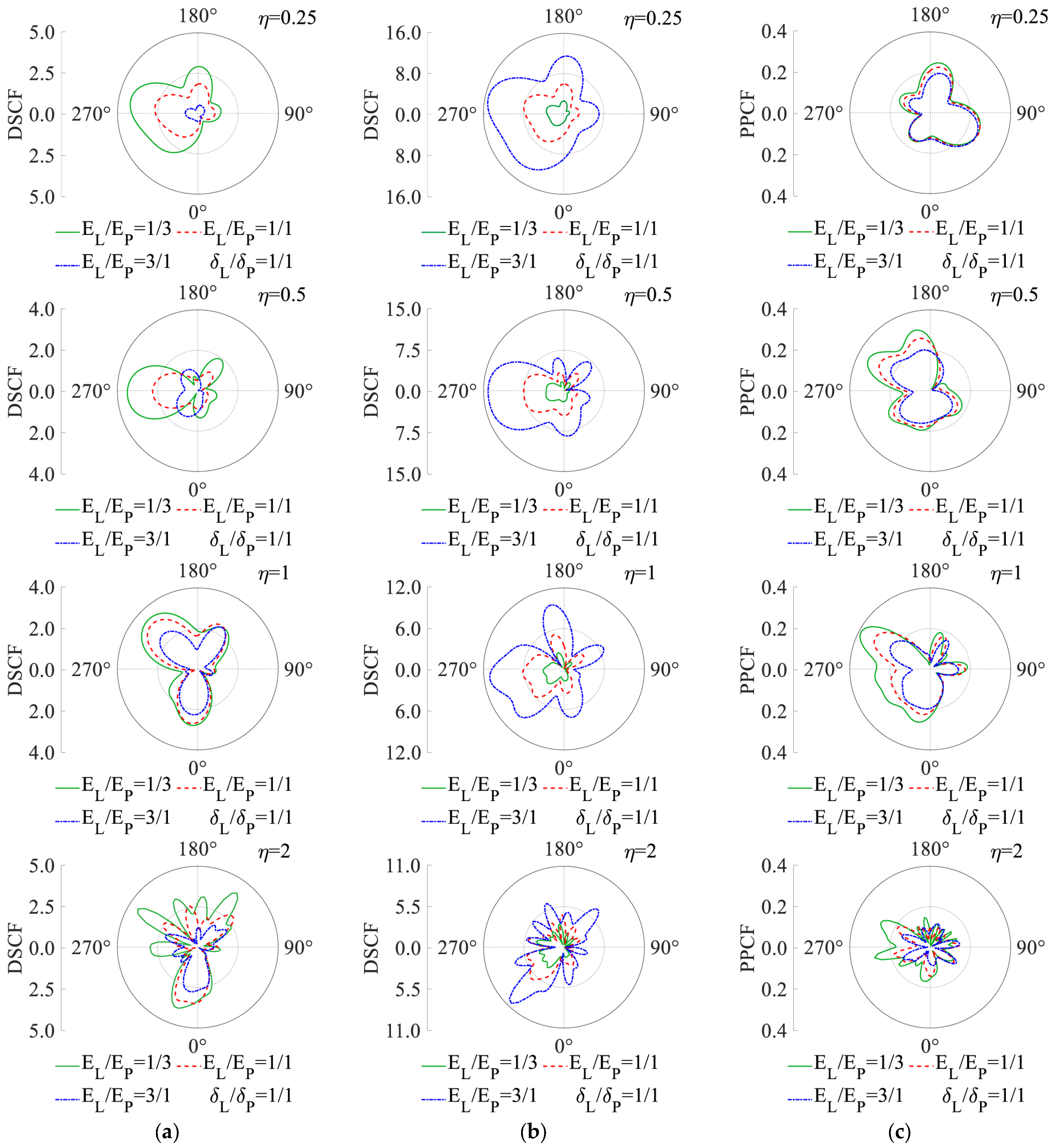
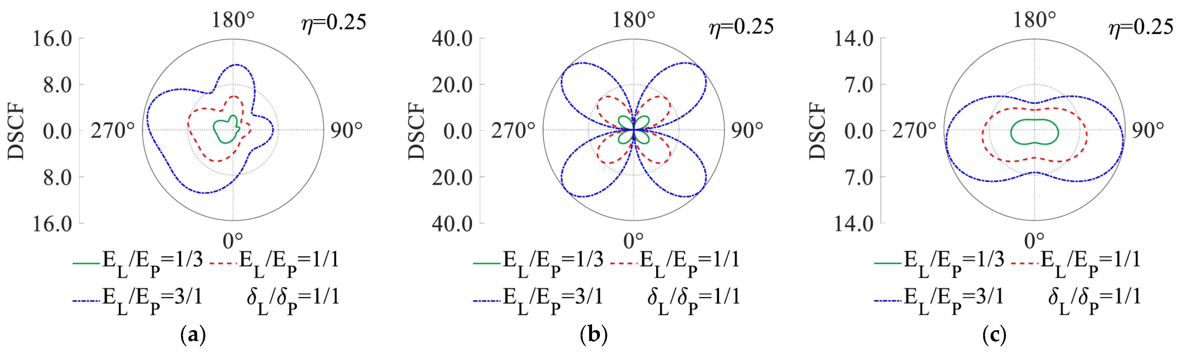
Incident frequency governs both the spatial distribution and magnitude of DSCFs and PPCFs. Low-to-medium frequencies (η = 0.25–0.5) amplify stress concentrations at the lining crown (DSCF = 7.2–12.1) and sidewalls (DSCF = 14.2–15.9), while high frequencies (η ≥ 1) shift stress peaks to the invert and foot arch regions (DSCF = 9.6–10.9). PPCF magnitudes diminish by 30% to 50% as frequency η increases from 0.25 to 2, reflecting attenuated pore pressure coupling at shorter wavelengths.

(2)

Enhancing the stiffness ratio between the lining and grouting zones can markedly reduce the DSCF and PPCF of the grouting area, while substantially escalating the DSCF of the lining. Furthermore, beyond a specific amplitude (E_L/E_P > 4), the lining DSCF amplifies by 80% in low-to-medium frequency and the seismic mitigation impact on the pore pressure is constrained in high frequency, while E_L/E_P < 2 inadequately meets the anti-liquefaction demand for pore pressure may increase several times. Thus, a stiffness ratio of two to four balances stress mitigation and structural practicality.

(3)

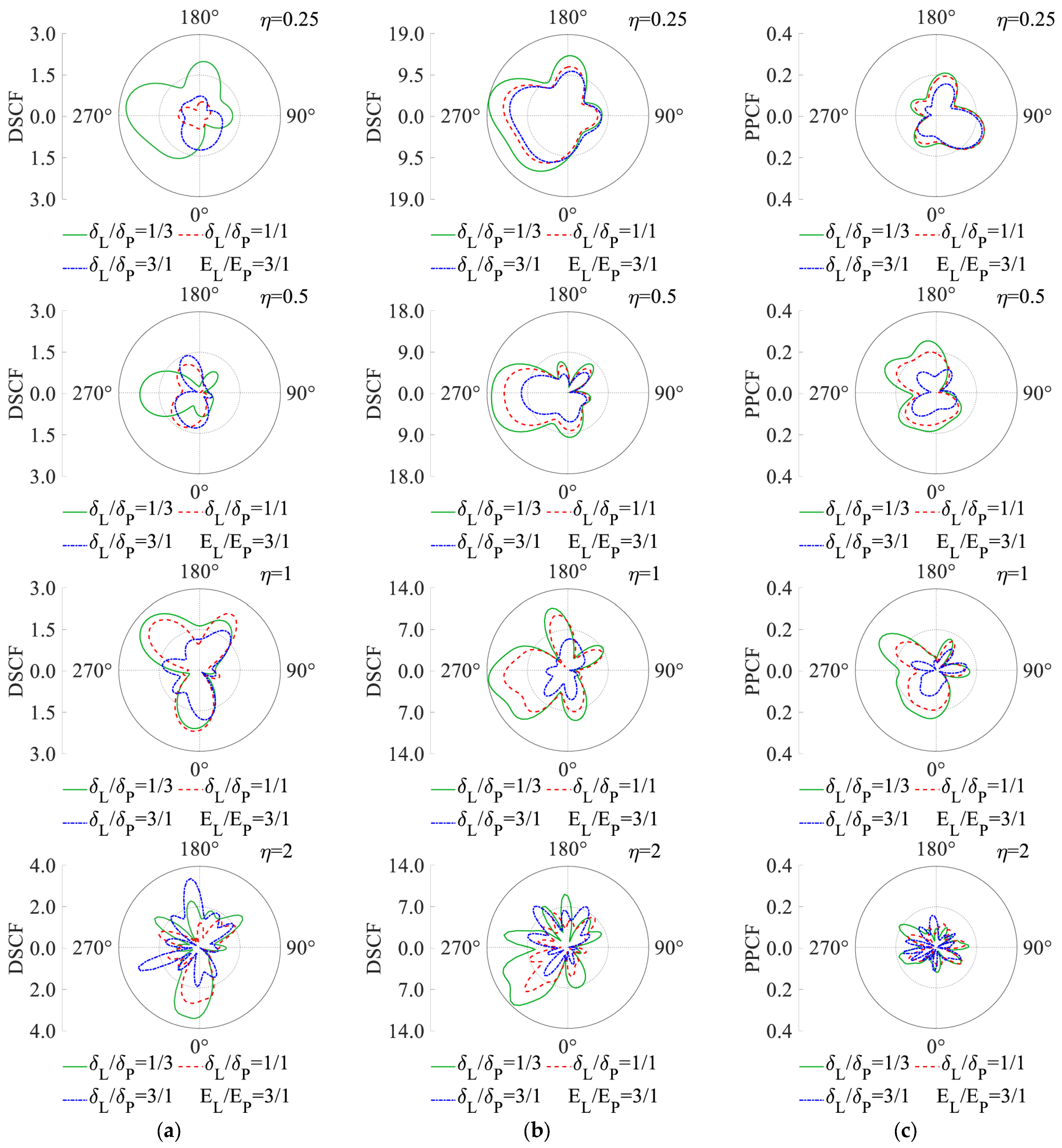
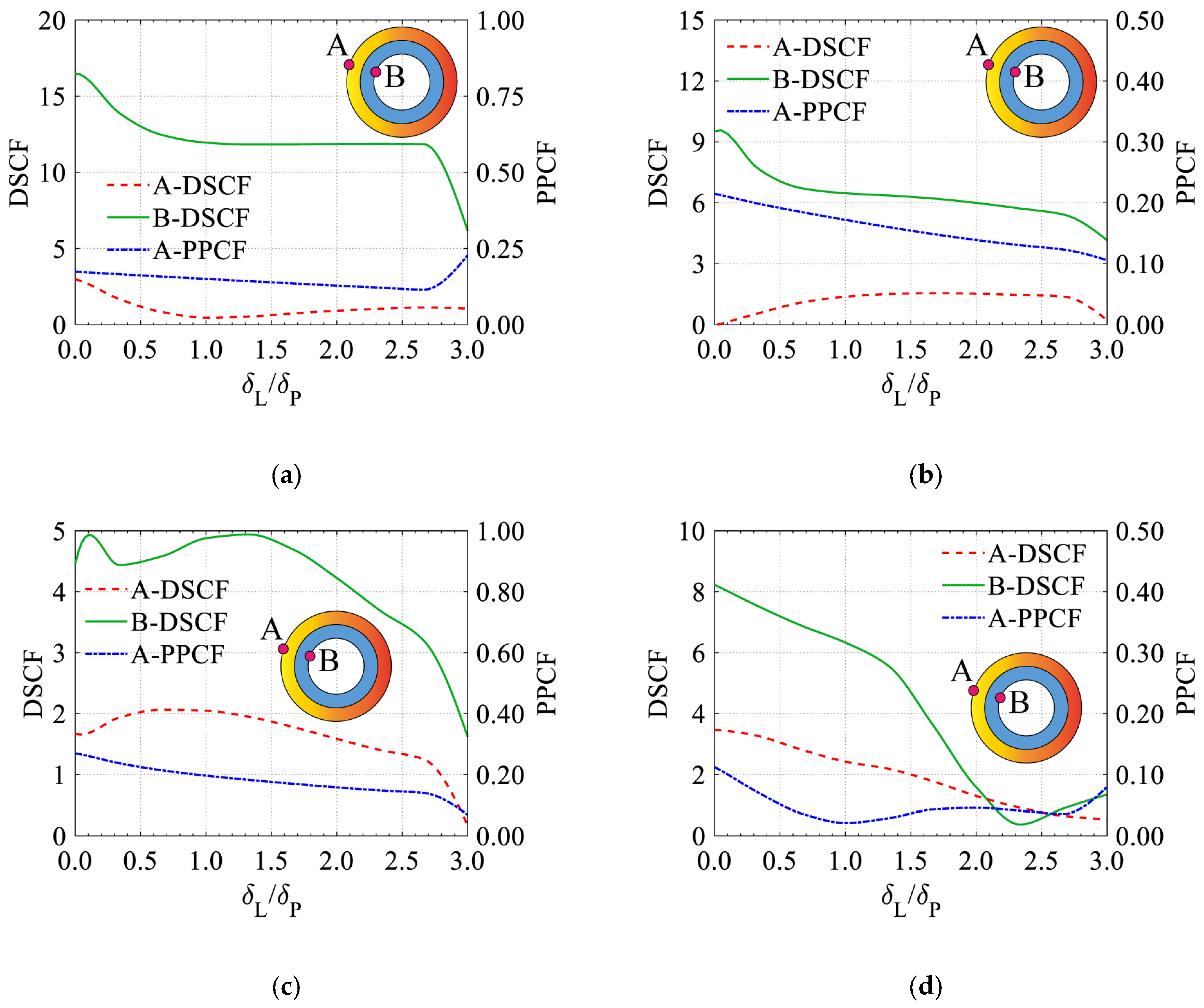
Augmenting the thickness ratio between the lining and grouting zones can effectively limit both the DSCF and PPCF of the soil in the grouting diffusion zone, while also partially reducing the DSCF of the lining. Nonetheless, above a specific amplitude (δ_L/δ_P > 2), the influence on the seismic mitigation efficacy of the lining stress is constrained. The thickness ratio is advised to be within the range of one to two.

(4)

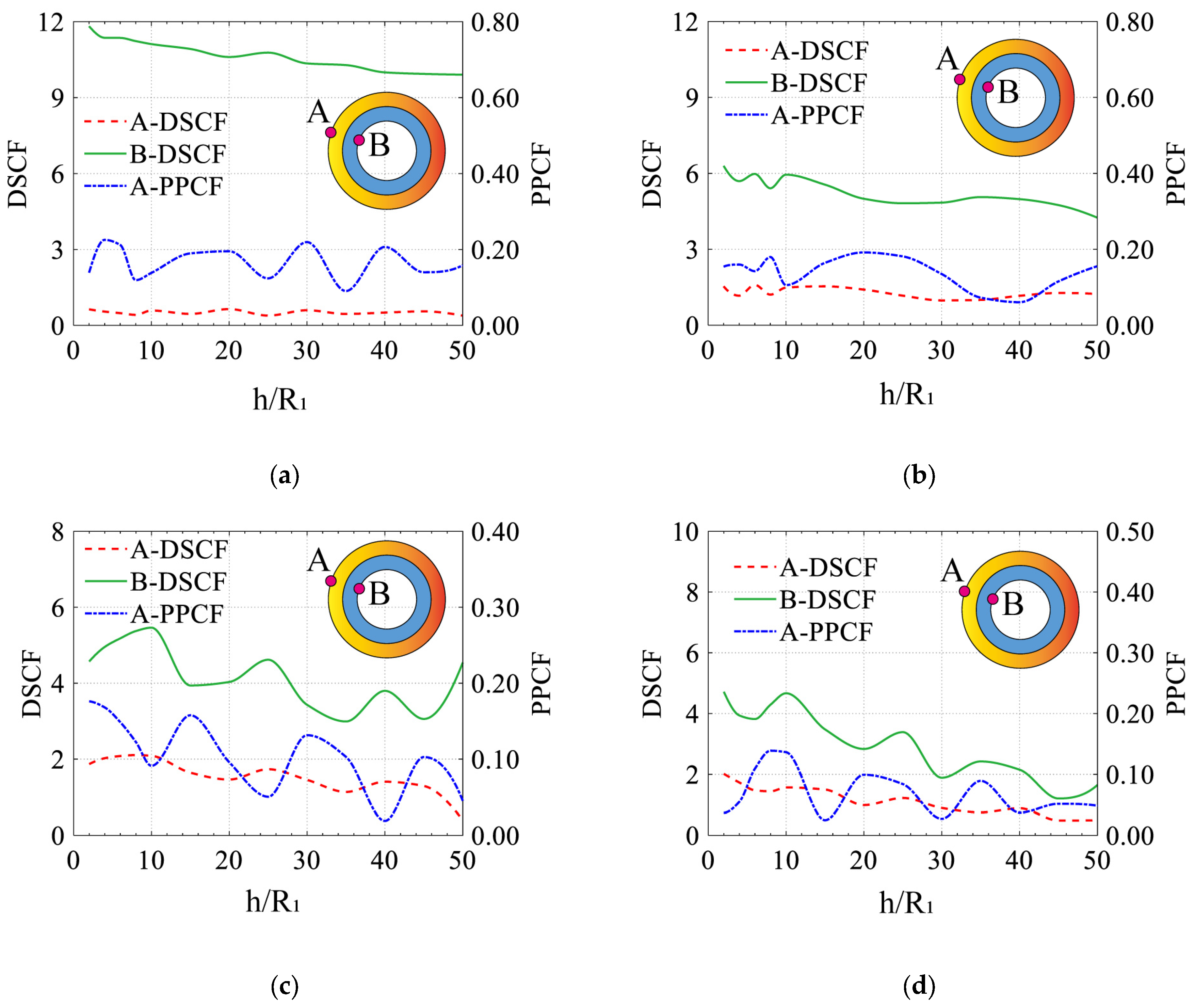
Shallow tunnels (h/R₁ < 5) exhibit pronounced R-wave-induced stress amplification (peak DSCF = 6.2–11.9 in low-to-mid frequency), with diminishing effects as depth increases (h/R₁ > 10). Medium-to-high frequencies (η ≥ 1) induce oscillatory DSCF and PPCF attenuation with depth, underscoring the vulnerability of shallow tunnels to surface wave dominance.

The DSCF distribution patterns derived from the suggested model in this study may unequivocally serve as a guideline for tunnel safety design.

6. Limitations and Future Work

This study employs simplified assumptions to enable analytical solutions, including linear poroelasticity (neglecting soil nonlinearity and plastic deformation), inviscid pore fluid (omitting energy dissipation via fluid viscosity), and homogeneous saturated soil conditions (excluding heterogeneity or partial saturation effects). The tunnel-grouting system is idealized as concentric cylindrical geometry under two-dimensional plane strain, which limits direct applicability to irregular configurations. While these assumptions ensure tractability, they preclude modeling of real-world complexities such as soil layering, multiphase fluids, or longitudinal wave interactions. Future studies should integrate viscoelastic damping and nonlinear constitutive laws to capture energy dissipation and large-strain behavior. Advanced numerical methods (e.g., three-dimensional finite element modeling) could address arbitrary geometries and multidimensional wavefields, while field validations using instrumented tunnels would enhance practical relevance. Further exploration of frequency-dependent grouting optimization and gas-liquid interactions in partially saturated soils could broaden the framework’s applicability to diverse geological and seismic scenarios. These extensions aim to align theoretical predictions with the multifaceted challenges of real-world tunnel engineering.

References

1. Yashiro, K.; Kojima, Y.; Shimizu, M. Historical earthquake damage to tunnels in Japan and case studies of railway tunnels in the 2004 Niigata ken-Chuetsu earthquake. Q. Rep. RTRI 2007, 48, 136–141. [Google Scholar] [CrossRef]
2. Huo, H.; Bobet, A.; Fernández, G.; Ramírez, J. Load transfer mechanisms between underground structure and surrounding ground: Evaluation of the failure of the Daikai station. J. Geotech. Geoenviron. Eng. 2005, 131, 1522–1533. [Google Scholar] [CrossRef]
3. Shen, Y.; Gao, B.; Yang, X.; Tao, S. Seismic damage mechanism and dynamic deformation characteristic analysis of mountain tunnel after Wenchuan earthquake. Eng. Geol. 2014, 180, 85–98. [Google Scholar] [CrossRef]
4. Pao, Y.H.; Mow, C.C.; Achenbach, J.D. Diffraction of elastic waves and dynamic stress concentrations. J. Appl. Mech. 1973, 40, 213–219. [Google Scholar] [CrossRef]
5. Lee, V.W. On deformation of near a circular underground cavity subjected to incident plane P waves. Eur. J. Earthq. Eng. 1993, 7, 29–35. [Google Scholar]
6. Lee, V.W.; Cao, H. Diffraction of SV Waves by Circular Canyons of Various Depths. J. Eng. Mech. 1989, 115, 2035–2056. [Google Scholar] [CrossRef]
7. Davis, C.A.; Lee, V.W.; Bardet, J.P. Transverse response of underground cavities and pipes to incident SV waves. Earthq. Eng. Struct. Dyn. 2001, 30, 383–410. [Google Scholar] [CrossRef]
8. Luo, H.; Lee, V.W.; Liang, J. Anti-plane (SH) waves diffraction by an underground semi-circular cavity: Analytical solution. Earthq. Eng. Eng. Vib. 2010, 9, 385–396. [Google Scholar] [CrossRef]
9. Xu, H.; Li, T.B.; Li, L.Q. Research on dynamic response of underground circular lining tunnel under the action of P waves. Appl. Mech. Mater. 2011, 99–100, 181–189. [Google Scholar] [CrossRef]
10. Li, Y.S.; Li, T.B.; Zhang, X. Response of shallow-buried circular lining tunnel to incident P wave. Appl. Mech. Mater. 2012, 160, 331–336. [Google Scholar] [CrossRef]
11. LIN, C. Wave Propagation in a Poroelastic Half-Space Saturated with Inviscid Fluid; University of Southern California: Los Angeles, CA, USA, 2002. [Google Scholar]
12. Biot, M.A. Theory of Propagation of Elastic Waves in a Fluid-Saturated Porous Solid. I. Low-Frequency Range. J. Acoust. Soc. Am. 1956, 28, 168–178. [Google Scholar] [CrossRef]
13. Biot, M.A. Theory of Propagation of Elastic Waves in a Fluid-Saturated Porous Solid. II. Higher Frequency Range. J. Acoust. Soc. Am. 1956, 28, 179–191. [Google Scholar] [CrossRef]
14. Sve, C. Elastic wave propagation in a porous laminated composite. Int. J. Solids Struct. 1973, 9, 937–950. [Google Scholar] [CrossRef]
15. Mei, C.C.; Foda, M.A. Wave-induced responses in a fluid-filled poro-elastic solid with a free surfacea boundary layer theory. Geophys. J. Int. 1981, 66, 597–631. [Google Scholar] [CrossRef]
16. Mei, C.C.; Si, B.I.; Cai, D. Scattering of simple harmonic waves by a circular cavity in a fluidinfiltrated poro-elastic medium. Wave Motion 1984, 6, 265–278. [Google Scholar] [CrossRef]
17. Li, W.; Zhu, S.; Lee, V.W.; Shi, P.; Zhao, C. Scattering of plane SV-waves by a circular lined tunnel in an undersea saturated half-space. Soil Dyn. Earthq. Eng. 2022, 153, 107064. [Google Scholar] [CrossRef]
18. Li, J.; Shan, Z.; Li, T.; Jing, L. Effects of the fluid-solid interface conditions on the dynamic responses of the saturated seabed during earthquakes. Soil Dyn. Earthq. Eng. 2023, 165, 107728. [Google Scholar] [CrossRef]
19. Xiang, G.; Tao, M.; Zhao, R.; Zhao, H.; Memon, M.B.; Wu, C. Dynamic response of water-rich tunnel subjected to plane P wave considering excavation induced damage zone. Undergr. Space 2024, 15, 113–130. [Google Scholar] [CrossRef]
20. Kattis, S.E.; Beskos, D.E.; Cheng, A.H.D. 2D dynamic response of unlined and lined tunnels in poroelastic soil to harmonic body waves. Earthq. Eng. Struct. Dyn. 2003, 32, 97–110. [Google Scholar] [CrossRef]
21. Hasheminejad, S.M.; Mehdizadeh, S. Acoustic radiation from a finite spherical in fluid near a poroelastic sphere. Arch. Appl. Mech. 2004, 74, 59–74. [Google Scholar] [CrossRef]
22. Hasheminejad, S.M.; Badsar, S.A. Elastic Wave Scattering by Two Spherical Inclusions in a Poroelastic Medium. J. Eng. Mech. 2005, 131, 953–965. [Google Scholar] [CrossRef]
23. Wu, D.; Gao, B.; Shen, Y.; Zhou, J.; Chen, G. Damage evolution of tunnel portal during the longitudinal propagation of Rayleigh waves. Nat. Hazards 2015, 75, 2519–2543. [Google Scholar] [CrossRef]
24. Gregory, R.D. The propagation of waves in an elastic half-space containing a cylindrical cavity. Math. Proc. Camb. Philos. Soc. 1970, 67, 689. [Google Scholar] [CrossRef]
25. Höllinger, F.; Ziegler, F. Scattering of pulsed Rayleigh surface waves by a cylindrical cavity. Wave Motion 1979, 1, 225–238. [Google Scholar] [CrossRef]
26. Luco, J.E.; de Barros, F.C.P. Dynamic displacements and stresses in the vicinity of a cylindrical cavity embedded in a half-space. Earthq. Eng. Struct. Dyn. 1994, 23, 321–340. [Google Scholar] [CrossRef]
27. Liu, Q.; Zhao, M.; Wang, L. Scattering of plane P, SV or Rayleigh waves by a shallow lined tunnel in an elastic half space. Soil Dyn. Earthq. Eng. 2013, 49, 52–63. [Google Scholar] [CrossRef]
28. Narayan, J.P.; Kumar, D.; Sahar, D. Effects of complex interaction of Rayleigh waves with tunnel on the free surface ground motion and the strain across the tunnellining. Nat. Hazards 2015, 79, 479–495. [Google Scholar] [CrossRef]
29. Zhang, Y.; Bai, S.; Borjigin, M. Internal force of a tunnel lining induced by seismic Rayleigh wave. Tunn Undergr Space Technol 2018, 72, 218–227. [Google Scholar] [CrossRef]
30. Cao, C.; Fang, X.; Zhu, C. Effects of a semi-circular valley on dynamic response of shallow tunnel with imperfect interface under Rayleigh wave incidence. Soil Dyn. Earthq. Eng. 2025, 190, 109204. [Google Scholar] [CrossRef]
31. Tan, Y.; Yang, M.; Li, X. Dynamic response of a circular lined tunnel with an imperfect interface embedded in the unsaturated poroelastic medium under P wave. Comput. Geotech. 2020, 122, 103514. [Google Scholar] [CrossRef]
32. Ding, H.B.; Tong, L.H.; Xu, C.J.; Zhao, X.S.; Nie, Q.X. Dynamic responses of shallow buried composite cylindrical lining embedded in saturated soil under incident P wave based on nonlocal-Biot theory. Soil Dyn. Earthq. Eng. 2019, 121, 40–56. [Google Scholar] [CrossRef]
33. Ding, H.; Tong, L.H.; Xu, C.; Hu, W. Aseismic Performance Analysis of Composite Lining Embedded in Saturated Poroelastic Half Space. Int. J. Geomech. 2020, 20, 4020156. [Google Scholar] [CrossRef]
34. Cedergren, H.R. Seepage, Drainage, and Flow Nets, 3rd ed.; Wiley: New York, NY, USA, 1989. [Google Scholar]
35. Terzaghi, K.; Peck, R.B. Soil Mechanics in Engineering Practice, 2nd ed.; Wiley: New York, NY, USA, 1948. [Google Scholar]
36. Lin, C.H.; Lee, V.W.; Trifunac, M.D. The reflection of plane waves in a poroelastic half-space saturated with inviscid fluid. Soil Dyn. Earthq. Eng. 2005, 25, 205–223. [Google Scholar] [CrossRef]
37. Zhang, C.; Liu, Q.; Deng, P. Surface Motion of a Half-Space with a Semicylindrical Canyon under P, SV, and Rayleigh Waves. Bull. Seismol. Soc. Am. 2017, 107, 809–820. [Google Scholar] [CrossRef]
38. Song, X.; Gu, H.; Zhang, X.; Liu, J. Pattern search algorithms for nonlinear inversion of high-frequency Rayleigh-wave dispersion curves. Comput. Geosci-uk 2008, 34, 611–624. [Google Scholar] [CrossRef]
39. GB 50446-2017; Code for Construction and Acceptance of Shield Tunneling Method. Ministry of Housing and Urban Rural Development of the People’s Republic of China & AQSIQ: Beijing, China, 2017.
40. Liang, J.H. Study on the Proportion of Backfill-Grouting Materials and Grout Deformation Properties of Shield Tunnel; Hehai University: Nanjing, China, 2006. [Google Scholar]
41. Zhang, H. Study on the Proportioning of Tail Void Grouting Material and up Floating Control of Shield Tunnel; Tongji University: Shanghai, China, 2007. [Google Scholar]
42. Wang, C.; Gou, C. Spherical cavity pressure filtration expansion model of the backfilled grouts in shield tunnel. J. Railway Sci. Eng. 2017, 14, 2670–2677. [Google Scholar]
43. Yang, Q.; Geng, P.; Wang, J.; Chen, P.; He, C. Research of asphalt–cement materials used for shield tunnel backfill grouting and effect on anti-seismic performance of tunnels. Constr. Build. Mater. 2022, 318, 125866. [Google Scholar] [CrossRef]
44. Zhang, J.X.; Zhang, N.; Zhou, A.; Shen, S.L. Numerical evaluation of segmental tunnel lining with voids in outside backfill. Undergr. Space 2022, 7, 786797. [Google Scholar] [CrossRef]
45. Fan, K. Scattering of Elastic Waves by Composite Lining of Shallow Buried Tunnel in Saturated Stratum; Southwest Jiaotong University: Chengdu, China, 2021. [Google Scholar]
Figure 1. Schematic representation of a grout-reinforced shallow tunnel lining in saturated soil under Rayleigh wave excitation: Coordinate system and semi-infinite boundary approximation (dashed circular arch).
Buildings 15 01589 g001
Figure 2. Comparison of normalized displacements of surface with the reduced dynamic model by Luco et al. [26]. (a) horizontal displacements; (b) vertical displacements.
Buildings 15 01589 g002
Figure 3. Comparison of DSCFs and PPCFs with variable stiffnesses and incident frequencies. (a) DSCFs of grouting reinforcement zone; (b) DSCFs of tunnel lining; (c) PPCFs of grouting reinforcement zone.
Buildings 15 01589 g003
Figure 4. Comparison of DSCFs of tunnel lining with variable stiffnesses under low-frequency wave incidence [45]. (a) Rayleigh wave; (b) vertical incident SV wave; (c) vertical incident P wave.
Buildings 15 01589 g004
Figure 5. Seismic damage pattern of lining structure in shallow buried section of Longxi tunnel in Wenchuan earthquake [23]. (a) Falling blocks and water seepage of Longxi tunnel crown; (b) crown and spandrel cracks in Longxi tunnel.
Buildings 15 01589 g005
Figure 6. DSCFs of the lining and grouting zone and PPCFs of the surface of grouting circle versus the stiffness ratios under different input frequencies. (a) η = 0.25; (b) η = 0. 5; (c) η = 1.0; (d) η = 2.0.
Buildings 15 01589 g006
Figure 7. Comparison of DSCFs and PPCFs with variable thickness and incident frequencies. (a) DSCFs of grouting reinforcement zone; (b) DSCFs of tunnel lining; (c) PPCFs of grouting reinforcement zone.
Buildings 15 01589 g007
Figure 8. DSCFs of the lining and grouting zone and PPCFs of the surface of the grouting circle versus the thickness ratios under different input frequencies. (a) η = 0.25; (b) η = 0. 5; (c) η = 1.0; (d) η = 2.0.
Buildings 15 01589 g008
Figure 9. DSCFs of the lining and grouting zone and PPCFs of the surface of the grouting circle versus the normalized depths under different input frequencies. (a) η = 0.25; (b) η = 0. 5; (c) η = 1.0; (d) η = 2.0.
Buildings 15 01589 g009
Disclaimer/Publisher’s Note: The statements, opinions and data contained in all publications are solely those of the individual author(s) and contributor(s) and not of MDPI and/or the editor(s). MDPI and/or the editor(s) disclaim responsibility for any injury to people or property resulting from any ideas, methods, instructions or products referred to in the content.