Future Climate Projections and Uncertainty Evaluations for Frost Decay Exposure Index in Norway

Abstract

To implement the geographical and future climate adaptation of building moisture design for building projects, practitioners need efficient tools, such as precalculated climate indices to assess climate loads. Among them, the Frost Decay Exposure Index (FDEI) describes the risk of freezing damage for clay bricks in facades. Previously, the FDEI has been calculated for 12 locations in Norway using 1961–1990 measurements. The purpose of this study is both updating the FDEI values with new climate data and future scenarios and assessing how such indices may be suitable as a climate adaptation tool in building moisture safety design. The validity of FDEI as an expression of frost decay potential is outside the scope of this study. Historical data from the last normal period as well as future estimated climate data based on 10 different climate models forced by two emission scenarios (representative concentration pathways 4.5 and 8.5) have been analyzed. The results indicate an overall decline in FDEI values on average, due to increased winter temperatures leading to fewer freezing events. Further, the variability between climate models and scenarios necessitates explicit uncertainty evaluations, as single climate model calculations may result in misleading conclusions due to high variability between models.

1. Introduction

1.1. Background

A changing climate creates the need for tools to assess building envelope performance under future climatic conditions [1]. Research has shown that the availability of practical tools is a significant barrier for building climate adaptations [2,3]. Assessments using available local climate data are key, and due to ongoing climate change, the need to adapt to future climate developments must also be addressed [4]. The development of tools addressing this is therefore key to implementing adaptation measures in practical building design and, thus, reducing building damages [4,5]. In this context, climate indices have been introduced in Norway and in countries with similar climates as a tool for practitioners to guide design choices in adapting to the local climate [6,7,8,9].

Lisø et al. showed that using a climate index that combines sub-zero temperatures and precipitation for geographical locations is an effective tool to assess the risk of frost decay in a clay brick façade placed in a particular climate [10]. They developed a Frost Decay Exposure Index (FDEI) and calculated FDEI values for 12 locations in Norway using historical weather data. To evaluate the future development of FDEI in Norway, an analysis of future climate model results is necessary. This will introduce a higher level of uncertainty in the estimated index values, due to variations in climate model outputs and multiple emission scenarios to choose from.

The uncertainties added from climate models require careful evaluation to increase result confidence and may be partitioned into internal model variability, model response uncertainty and emission scenario forcing [11]. The uncertainties introduced by such forecasts should be explicitly communicated to the user of the index values, in order for the user to evaluate future climate loads when considering climate adaptation measures in building projects. These should include direct uncertainties associated with the prediction model as well as indirect uncertainties related to the strength of the knowledge supporting the assessment [12].

1.2. Objectives and Scope

To evaluate uncertainties introduced by future climate modeling when producing climate index value forecasts, an ensemble of climate models and scenarios are used. Quantified expressions of model output variability may thus accompany the index output values. Separating uncertainty expressions from the point estimates, rather than presenting average or derived values, increases the value of the index to the user by minimizing the loss of information [13].

The purpose of this study is twofold. First, we intend to update the original FDEI presented by Lisø et al. [10] to incorporate the climatic changes in Norway over the last normal period including future estimated developments. Second, we aim to investigate how climate indices may serve as moisture safety design tools to promote climate adaptation in building projects by using the FDEI as a case index. Project engineers responsible for moisture safety design need effective tools to implement climate adaptation in building design. The most common method for assessing moisture safety design in Norwegian building projects is qualitative risk assessments of design solutions [14]. By including quantitative expressions of local climate load variability and future climate load developments in the risk assessments, climate adaptation assessments may be included with minimal changes to the normal workflow for the Norwegian project engineer.

We therefore address the following research questions to explore the aims outlined above:

• How have the FDEI values developed in Norway over the last normal period, and what are the likely future developments?
• What additional uncertainties are introduced in the FDEI by using future climate projections?
• How can we use the FDEI and uncertainty information as design tools for moisture safety design in building projects?

To answer these questions, we have calculated FDEI values for 12 locations in Norway, both historical measurements (1991–2020) and future climate scenarios (2031–2060 and 2071–2100), using the models and methods described in Section 2. Section 3 presents the results, while Section 4 discusses the results and implications for the three research questions. An important limitation to the scope of this study is that material responses to absolute FDEI values are not considered nor is the validity of FDEI as an expression of frost decay potential. Wind is not included in FDEI even though the index considers frost decay exposure on facades, but advantages and disadvantages to this choice are outside the scope of this study. In light of these limitations, we thus consider the FDEI values to be frost load potentials for a given location. Further, when discussing research question 1, relative differences between locations and scenarios are evaluated rather than absolute index values.

1.3. Climate-Related Uncertainties

Norway’s climate varies widely in terms of temperature and precipitation. The coastal regions in western Norway are characterized by high annual normal precipitation, typically between 1000 and 3000 mm [15]. Conversely, the annual normal precipitation in the regions east of the mountainous areas and inner parts of Finnmark was recorded to be 300–800 mm during the same period. Temperature variations in Norway are also significant among different seasons and geographical locations. For the 1991–2020 period, the geographical variation in annual normal mean temperature is over 10 °C [16]. The term “normal” value for precipitation or temperature in this paper refers to the average value over a 30-year period, calculated according to the World Meteorological Organization (WMO) guidelines on the calculation of a climate normal [17]. The Norwegian Meteorological Institute’s report on standard models [18] and their report on regional climate division [19] offer a more detailed description of the Norwegian climate.

The FDEI describes the co-occurrence of two weather events: zero freezing-point crossings and prior precipitation. Given the geographical variability of weather patterns in Norway, carefully considering the uncertainties of the index itself is necessary. Future climate scenarios require contributions from socio-economic and meteorological research to produce emission scenarios and climate models. However, these underlying models introduce a higher level of uncertainty into the results compared to models using present-day climate [13]. To assess how future climate-induced uncertainties influence model outputs, the requirements for model comprehensiveness are high. The ambiguity and uncertainty associated with climate change information represent barriers to climate adaptation [20,21], by concealing the risks connected to inaction [22]. The uncertainties involved in determining future climate loads due to high problem complexity thus hinders the evaluation of benefits that could be derived from adaptation efforts [23]. Many decision makers in building projects perceive adaptation measures to increase costs owing to initial investments, with economic concerns being frequently reported in the literature as a key barrier to both climate adaptation and sustainability assessments [24,25]. The low availability of tools and methods to consider future climates in building moisture safety design is also a barrier to climate adaptation in building projects [14]. Tools and methods that reduce these uncertainties have proven to be important drivers for adaptation [2,26,27]. Additionally, increased information flows and awareness within building projects further facilitate the climate adaptation of building designs [28].

1.4. Climate-Based and Response-Based Indices

Both climate-based and response-based indices are challenging to integrate into a universally agreed assessment framework, due to factors such as problem complexity and the variability, uncertainties and interdependencies of the factors at play and determination of benchmarks [29]. Vanemeulenbroucke et al. have assessed the advantages and disadvantages of using response-based and climate-based indices. Response-based analysis requires more computational power and more predefinition but is also more precise due to the performance dependency on specific combinations of building parameters such as wall composition, material properties, etc. [30]. A further implication of this is that climate-based analyses produce a single value per location, and response-based analyses may produce a distribution as they may be based on a high number of parameter variations and thus promote quantitative uncertainty treatment of the results.

The drawback of pure climate-based indices is that they need to be validated and calibrated against the in situ response of a material or building part to estimate performance, as the response is not precalculated. An analysis of building defects in concert with the development of a relevant climate index is a way to mitigate this drawback, by connecting in situ performance to index values. A comprehensive analysis of masonry damage cases over a 20-year period by Kvande et al. showed that a large part of the cases could have been avoided if better methods for climate adaptation were available at the time of construction. They concluded in 2009 that there is a need to develop improved tools for project engineers to assist climate adaptation in building projects [31], a conclusion that is unfortunately still not sufficiently addressed today despite significant progress in the field of climate adaptation research [32].

1.5. Climate Adaptation of Buildings Using Precalculated Climate Indices and Qualitative Risk Analysis

The technical screening criteria in the EU Taxonomy Regulation for economic activities regarding the construction of new buildings requires building projects to carry out a climate risk and vulnerability assessment for chronic and acute climate-related hazards [33]. Thus, methods for evaluating the impact and future development of climate loads using climate indices may be a quick-to-use approach for the qualitative risk analysis required in the taxonomy.

Heat, air and moisture (HAM) simulation tools are sparingly used to study deterioration risks by project engineers. This is because climate-related uncertainties in the model are demanding to assess, and both model creation and result processing require significant effort [34]. Coupling climate indices that describe relevant climate stress levels with the risk assessments of the solution at hand, which requires less effort per evaluation, is often preferred by moisture design engineers under tight budget constraints [14]. To address this, the Klima 2050 research Centre in Norway has developed a framework for climate adaptation that highlights the need to geographically differentiate climate loads and take future climate trends into account. The framework is a tool meant to help project designers to incorporate climate adaptation in established workflows, by using qualitative risk assessment methods supported by climate assessment tools and resources [4].

2. Materials and Methods

2.1. Frost Decay Exposure Index (FDEI)

The FDEI combines temperature and precipitation to assess the climatic risk of frost damage in exposed porous building materials [10]. FDEI is the annual accumulated 4-day sum of precipitation prior to all freezing-point crossings (FPCs) in a year. The original index published by Lisø et al. [10] was created by analyzing historical climatic data (1961–1990) collected from 13 cities with differing local climates in Norway to characterize the risk of frost damage in porous building materials at each location. Temperature data were obtained from three time points each day (0600, 1200 and 1800) in addition to the daily maximum and minimum, to count the number of freezing-point crossings (FPCs) per year. The precipitation 4 days prior to each FPC was summed up and categorized as either snow or rain. The resulting FDEI was defined as the accumulated rain falling in the 4 days prior to all FPCs in a year. Symbolically, FDEI may be expressed as follows for a given location in a given year (Equation (1)):

$$FDEI=\sum _{{FPC}_m}{P}_{m,n}+P_{m,n-1}{+P}_{m,n-2}+P_{m,n-3}$$

(1)

where P is daily precipitation in [mm], and n is the day of FPC number m. The usefulness of the FDEI as a tool to assess the risk of frost decay was later confirmed by Pakkala et al. [35] through their work on Finnish concrete façades and Mandinec and Johansson’s parameter study of a Swedish brick façade [36]. Derivatives of FDEI were evaluated by the latter, in order to account for the effects of wind-driven rain and solar radiation; however, the simpler version of FDEI originally developed by Lisø et al. was found to describe the risk of frost decay in bricks more accurately by the same authors [36].

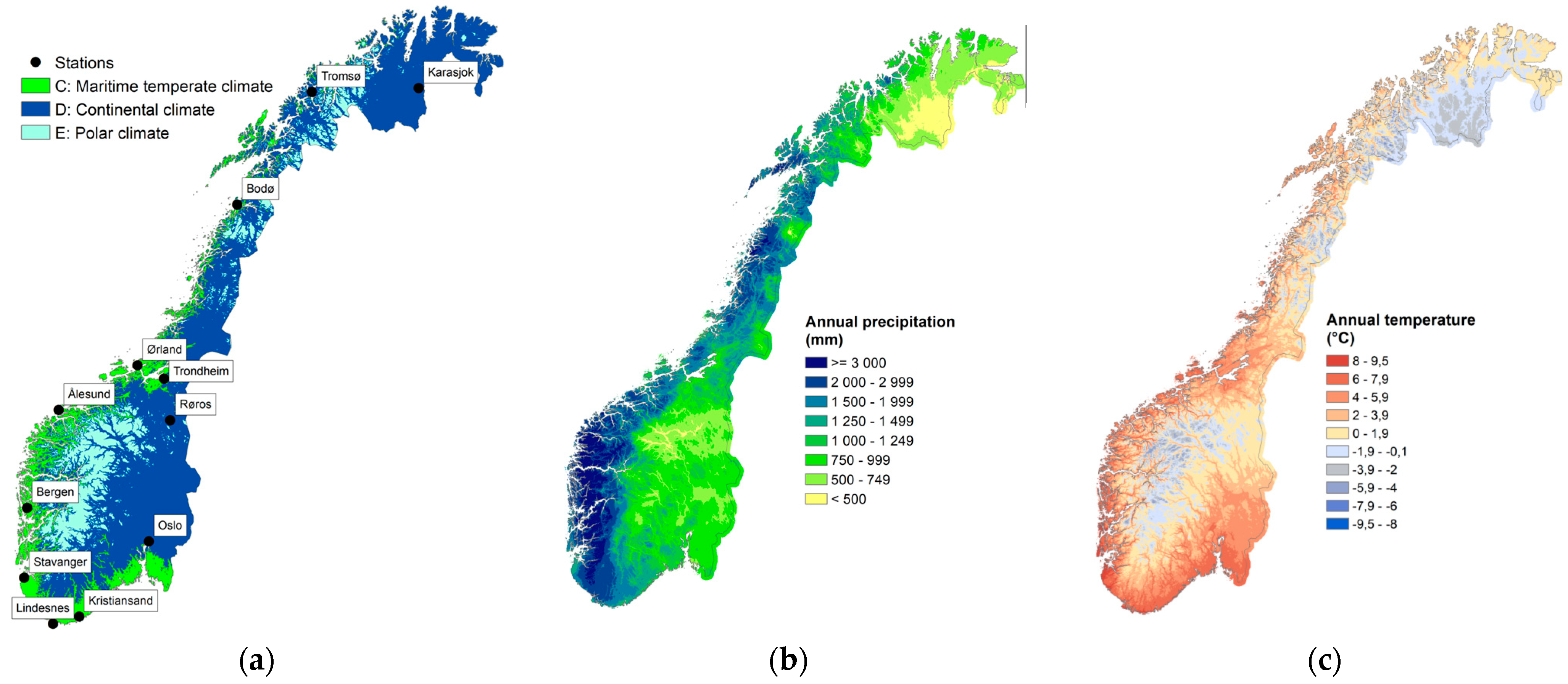
2.2. Locations and Climate Variations

The geography and topography of Norway are diverse, stretching from 58 to 71° N, with great contrasts between coastal, mountainous and inland regions. Thus, the climate type varies significantly over relatively short distances, from maritime temperate (C) along the coast to continental (D) and polar (E) climates in inland and northern regions, when classified following the Köppen–Geiger climate system [37] (Figure 1). Coastal regions experience high precipitation and mild winters, whereas inland regions are drier and reach colder temperatures. The locations studied in this paper are chosen to reflect this diversity, covering a large range of Norway’s variation in precipitation and temperature.

Twelve stations located at points from Lindesnes (south) to Karasjok (north) were selected. Due to data quality in the available measurements, two of the locations from the original study by Lisø et al. [10] were excluded (Fruholmen and Lyngdal), and one new location was included (Lindesnes). The station names, numbers and locations (latitude and longitude) are listed in

Table 1. Station data and annual normal temperature and precipitation in the last and current normal periods, listed in order from the southmost to the northmost station. The data were obtained from The Norwegian Meteorological Institute [27].

Station Name	Station Number	Latitude	Longitude	Annual Normal Temperature (1961–1990)	Annual Normal Temperature (1991–2020)	Annual Normal Precipitation (1961–1990)	Annual Normal Precipitation (1991–2020)
Lindesnes	SN41770	57.9815	7.048	7.4	8.6	1159	1245
Kristiansand	SN39040	58.2000	8.0767	6.6	7.6	1299	1384
Stavanger	SN44560	58.8843	5.637	7.4	8.4	1180	1257
Oslo	SN18700	59.9423	10.72	5.7	7.0	763	837
Bergen	SN50540	60.383	5.3327	7.6	8.4	2250	2496
Ålesund	SN60990	62.5617	6.115	6.9	7.9	1310	1451
Røros	SN10380	62.5773	11.3518	0.3	1.1	504	531
Trondheim	SN69100	63.4597	10.9305	5.3	6.1	892	823
Ørland	SN71550	63.7045	9.6105	5.8	6.8	1048	994
Bodø	SN82290	67.2723	14.3816	4.5	5.5	1020	1118
Tromsø	SN90450	69.6537	18.9368	2.5	3.4	1031	1091
Karasjok	SN97251	69.4635	25.5023	−2.4	−1.2	366	417

alongside measured annual normal temperature and normal precipitation for the periods 1961–1990 and 1991–2020. The data from all stations were obtained from The Norwegian Meteorological Institute (MET) [38]. All stations follow WMO’s requirements for measurement location [17] (although some are not formally classified as such). For exposure category and performance category for the stations, see station information published by MET [38]. The Urban Heat Island effect was studied in Venter et.al., 2020 [39], which showed that expanding and keeping green areas in Oslo helps to reduce the highest temperatures. The station in Oslo is not in the city center and is not affected by the UHI effect. Other stations in the biggest cities are located along the coast or so far north that UHI effects are negligible.

2.3. Temporal Resolution of Historical Measurements

The daily maximum (T_max) and minimum (T_min) temperatures can be used to determine whether an FPC occurred on a given day. We combined these data with daily precipitation measurements to obtain the index values. FPCs were recorded for days when the T_max was positive and T_min was negative. A disadvantage of using daily maximum and minimum values is that it registers zero crossings in both directions—warm to cold and cold to warm—thus, it is unknown if freezing, thawing or both occurs and if more than one freezing event occurs in one day.

Therefore, synoptic and hourly measurement values were also included for the historical scenario, to assess the impact of temporal resolution in the models. Historically, synoptic measurements of meteorological elements such as temperature and precipitation were taken three times a day, in the morning, at midday and in the evening (0600, 1200 and 1800 UTC). In the 1990s and 2000s, automated measurements were implemented for most stations, resulting in higher temporal resolutions of the data (i.e., Oslo in 1992 and Tromsø in 2003). Currently, weather elements can be studied on an hourly timescale for all the included stations, which ensures that freezing events are recorded when temperatures change from positive to negative.

Nevertheless, using daily data has several advantages. A higher number of stations measure T_max and T_min compared to hourly data. In addition, gridded maps are available for daily data, which cover all of Norway from 1957 to the present day [40,41]. Finally, a comparison to future climate scenarios is available, as these are based on daily data.

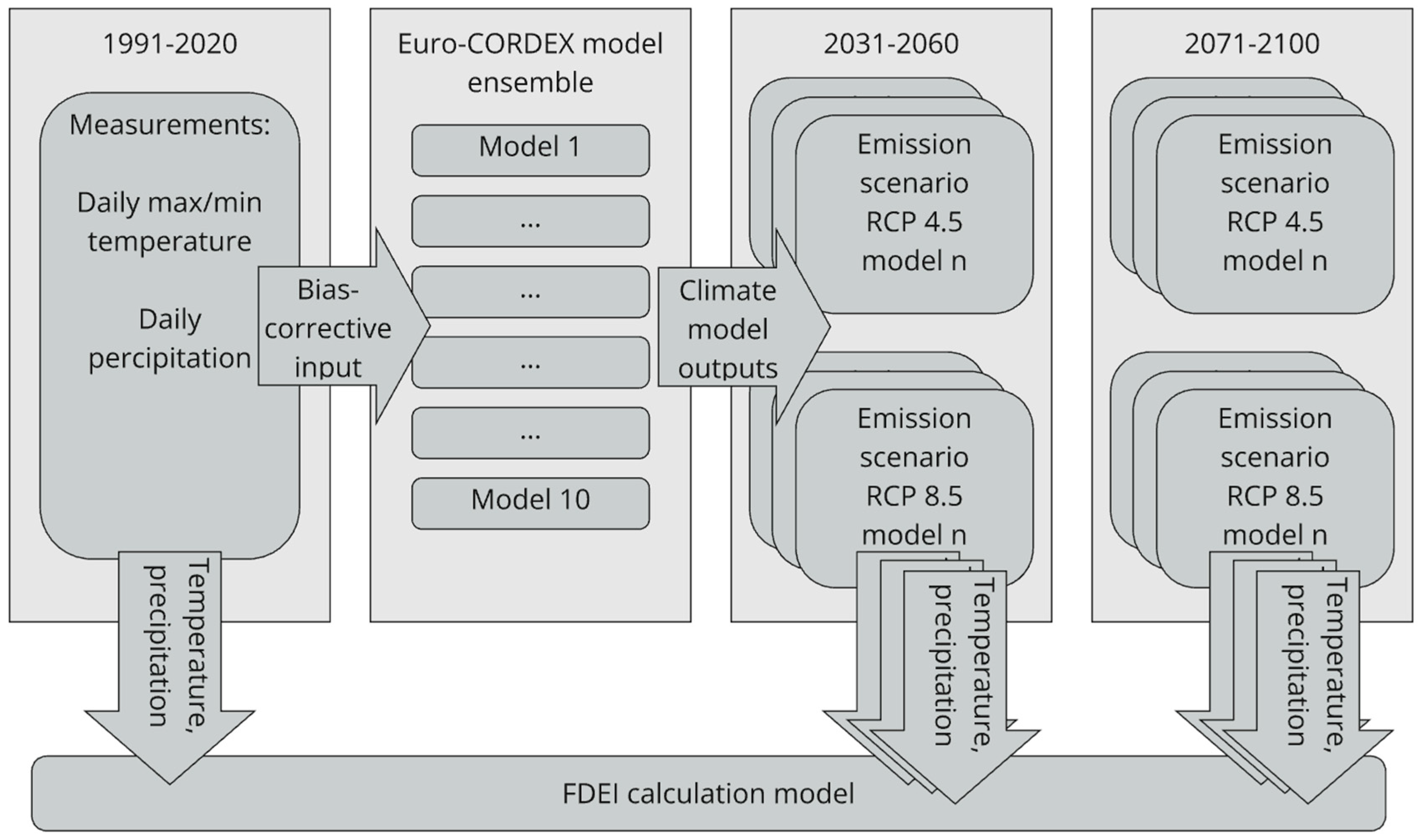
2.4. Future Climate Scenarios

To study future changes in the FDEI, we used downscaled, bias-adjusted climate projections of T_max, T_min and precipitation on a 1 × 1 km grid. The data were obtained from the Norwegian Centre for Climate Services [38]. The bias-adjustment and downscaling methods for T_max, T_min and precipitation are described by Wong in earlier studies [42,43]. The variables were bias-adjusted using an empirical quantile mapping method preserving the change signals and using 1 km gridded data derived from observations for the period 1971–2000 as reference.

The high-resolution climate projections were based on a selection of ten regional climate model (RCM) simulations from the EURO-CORDEX initiative [44]. The selected models are listed in

Table 2. Global climate model and regional climate model combinations from EURO-CORDEX [44].

Institute	Global Climate Model (GCM)	Regional Climate Model (RCM)	Combination
Climate Limited-area Modelling Community	CNRM-CM5	CCLM-4-8-17	CNRM_CCLM
Swedish Meteorological and Hydrological Institute	CNRM-CM5	RCA4	CNRM_RCA
Climate Limited-area Modelling Community	EC-EARTH	CCLM4-8-17	EC-venterEARTH_CCLM
Danish Meteorological Institute	EC-EARTH	HIRHAM5	EC-EARTH_HIRHAM
Royal Netherlands Meteorological Institute	EC-EARTH	RACMO22E	EC-EARTH_RACMO
Swedish Meteorological and Hydrological Institute	EC-EARTH	RCA4	EC-EARTH_RCA
Swedish Meteorological and Hydrological Institute	HadGEM2-ES	RCA4	HADGEM_RCA
Swedish Meteorological and Hydrological Institute	IPSL-CM5A-MR	RCA4	IPSL_RCA
Climate Limited-area Modelling Community	MPI-ESM-LR	CCLM	MPI_CCLM
Swedish Meteorological and Hydrological Institute	MPI-ESM-LR	RCA4	MPI_RCA

; the rightmost column lists the names used in this article, which combine the global climate model (GCM) used to provide the boundary data with the RCM itself. Two representative concentration pathways (RCPs)—RCP4.5 and RCP8.5—were used [45]. Hence, both medium- and high-emission scenarios were used to study changes in the middle (2031–2060) and end (2071–2100) of the century compared to the reference period 1991–2020 (current climate normal period).

2.5. Evaluation and Analysis Methodology

The T_max, T_min and daily precipitation values were extracted from the 12 locations listed in Table 1. The latitude and longitude at each station were used to extract a time-series of daily values from the closest grid point, which was used to calculate the FDEI. Note that the historical part from the RCM data from EURO-CORDEX only covers the period until 2005, while the years from 2006 onward are covered by future projections. Thus, to obtain data for the reference period 1991–2020, data from the historical RCM simulations were combined with future scenarios for 2006–2020 under both the medium- (RCP4.5) and high- (RCP8.5) emission scenarios. This was performed for each model in Table 2, after which changes in the FDEI were estimated for all 12 locations and 10 models, as illustrated in Figure 2. The changes between the control period (1991–2020) and future scenarios for the middle (2031–2060) and end (2071–2100) of the century for both emission scenarios—medium (RCP4.5) and high (RCP8.5)—were calculated.

To evaluate the representativeness of the climate model ensemble outputs with respect to temperature changes and relative precipitation changes, a comparison against the EURO-CORDEX CMIP5 ensemble was performed (see Figure 3).

To evaluate the method sensitivity with respect to temporal resolution and enable comparison between 1991–2020 and 1961–1990 results (see Figure 4), a temporal resolution bias factor must be identified. Lisø et al. [10] used a mix of daily max/min and synoptic hours to develop their index, depending on the data quality available at each location. While this mixed method may increase the precision of the 1961–1990 index, the method is difficult to reproduce. The temporal resolution bias factor describes the sensitivity of the results to temporal resolution, according to Equation (2).

$$K_{temporal resolution}={\displaystyle \frac{{FDEI}_{max/min}}{{FDEI}_{synoptic}}},$$

(2)

where $FDE{I}_{max/min}$ is the average calculated FDEI for all locations in the 1991–2020 data set using daily maximum and minimum temperatures, and $FDE{I}_{synoptic}$ is the same only using temperature readings at synoptic hours (0600, 1200, 1800).

3. Results

3.1. Evaluation of Climate Model Ensemble

Overall, the changes for both temperature and precipitation are larger in RCP8.5 than they are in RCP4.5 (Figure 3). For precipitation, the variability among both the selected models and interquartile range (IQR)—including the whisker—of the whole ensemble increases from RCP4.5 to RCP8.5. The selected models all lie within the whiskers of the boxplots, that is, there are no outliers compared with the entire ensemble. Further, the models cover the range of the whiskers well for temperature, indicating a good representation of the entire ensemble in terms of temperature changes. However, the selected models do not completely cover the lower end of the changes in the EURO-CORDEX ensemble for precipitation; specifically, none of the selected models show a decrease in precipitation.

Figure 3 shows the projected temperature and precipitation changes in Norway for the end of the 21st century (2071–2100) relative to the 1991–2020 reference period (spatially averaged from 1 × 1 km grid values). The figure shows the changes for the 10 selected RCM runs against all available EURO-CORDEX simulations for RCP4.5 and RCP8.5. Notably, while we used bias-adjusted data in this study, the climate change signals were conserved [34].

Among the RCMs, RCA4 shows the strongest signals for both temperature and precipitation, showing the largest changes among the EURO-CORDEX models. As RCA4 contributes to 5 out of 10 simulations, the median and IQR of the selected models are higher than those of the complete ensemble, particularly those of RCP8.5. The largest temperature changes are observed in the HadGEM downscaling, whereas the MPI-ESM-LR-driven simulations show the smallest warming. Temperature changes are more strongly influenced by the driving GCM than by the RCMs, but the RCMs could also result in considerable variance under RCP8.5. Conversely, precipitation changes are less influenced by the driving GCMs, which is in agreement with studies from other regions [46,47,48,49].

Figure 3. Temperature changes (a) and relative precipitation changes (b) spatially averaged over Norway in the EURO-CORDEX simulations used in this study (symbols) and from the complete EURO-CORDEX CMIP5 ensemble (box-plots). Different symbols denote different RCMs, while the position and labels on the x-axis indicate the driving GCMs and scenarios, respectively. The two RCP scenarios are shown in different colors. The numbers after the scenario names on the x-axis correspond to the number of available simulations in the entire EURO-CORDEX ensemble. A standard value of 1.5 times the interquartile range is used for the boxplots.

Figure 3. Temperature changes (a) and relative precipitation changes (b) spatially averaged over Norway in the EURO-CORDEX simulations used in this study (symbols) and from the complete EURO-CORDEX CMIP5 ensemble (box-plots). Different symbols denote different RCMs, while the position and labels on the x-axis indicate the driving GCMs and scenarios, respectively. The two RCP scenarios are shown in different colors. The numbers after the scenario names on the x-axis correspond to the number of available simulations in the entire EURO-CORDEX ensemble. A standard value of 1.5 times the interquartile range is used for the boxplots.

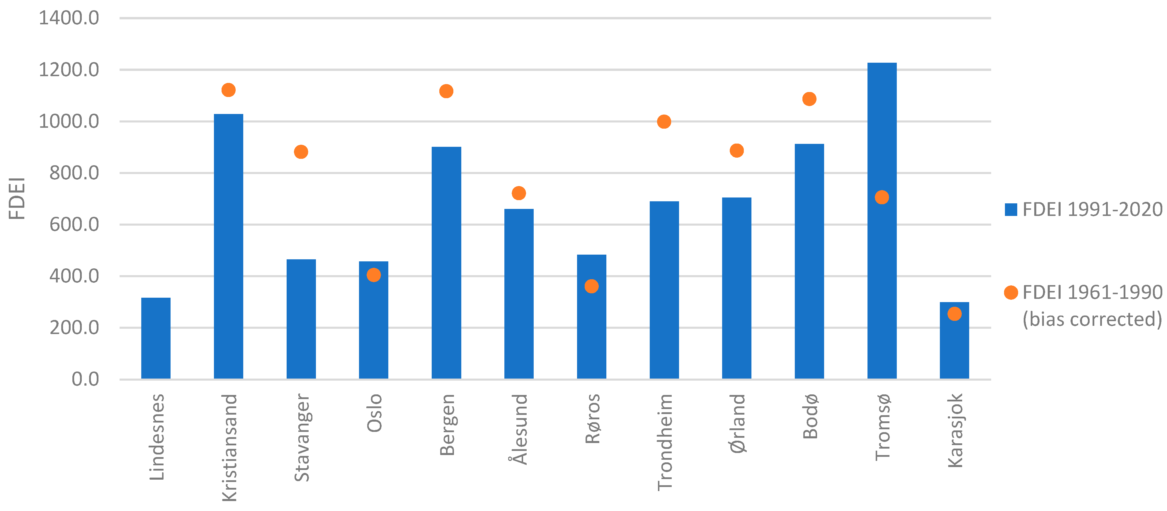
3.2. FDEI Based on Historical Observations (1991–2020)—Influence of Temporal Variations and Comparisons with 1961–1990 Data

The FDEI values for each location for the 1991–2020 period are presented in

Table 3. Average annual FDEI values for 4-day accumulated rainfall before each freezing event for the historical period 1991–2020, using three different temporal resolutions. Note that hourly values of temperature and precipitation are not available for the whole period; thus, period length differs between locations for this temporal resolution (e.g., 1992–2020 for Oslo and 2003–2020 for Tromsø).

	Lindesnes	Kristiansand	Stavanger	Oslo	Bergen	Ålesund	Røros	Trondheim	Ørland	Bodø	Tromsø	Karasjok
FDEImax/min 1	315.9	1027.4	464.8	456.9	900.4	659.9	483.1	689.5	703.9	911.8	1226.8	299.3
FDEIhourly	175.2	650.0	346.1	282.3	647.1	348.2	324.8	477.9	453.5	583.2	689.0	193.4
FDEISynoptic 2	144.2	488.0	234.1	248.5	525.1	243.6	222.2	348.1	319.2	402.8	551.9	135.3

¹ daily maximum and minimum temperatures, ² daily temperature readings at 0600, 1200 and 1800.

, with the corresponding FPC values presented in

Table 4. Average annual number of FPCs based on measurement data for the historical period 1991–2020, using three different temporal resolutions. Note that hourly values of temperature and precipitation are not available for the whole period; thus, period length differs between locations for this temporal resolution (e.g., 1992–2020 for Oslo and 2003–2020 for Tromsø).

	Lindesnes	Kristiansand	Stavanger	Oslo	Bergen	Ålesund	Røros	Trondheim	Ørland	Bodø	Tromsø	Karasjok
FPCmax/min 1	29.5	82.8	51.4	75.5	46.2	38.7	102.3	82.8	60.9	72.0	87.4	91.3
FPChourly	15.3	49.4	35.4	45.7	30.4	20.6	78.5	53.6	35.3	43.0	48.9	57.3
FPCSynoptic 2	13.2	38.5	25.5	38.6	26.6	14.7	58.3	40.0	25.5	29.4	36.8	38.8

¹ daily maximum and minimum temperatures, ² daily temperature readings at 0600, 1200 and 1800.

. The index value is influenced by the temporal resolution of the data, as evidenced when calculating FDEI based on (1) daily maximum/minimum (max/min) temperatures, (2) hourly temperatures and (3) synoptic hour temperatures (0600, 1200 and 1800). The daily max/min data produced higher FDEI values than those of the other two data sets for all locations. This occurred because there was no way of knowing whether zero crossing events represent a freezing event, a thawing event or both. Thus, all days with maximum temperatures above 0 °C and minimum temperatures below 0 °C were counted as freezing events. Furthermore, hourly values produced higher FDEI indices than those estimated using synoptic hours for all locations, likely because they may indicate more than one freezing event per day, which cannot be captured with only three measurements per day. The ratio between FDEI and FPC shows little change between the different temporal resolutions, indicating that FPC values are the parameter influencing the difference rather than precipitation.

As hourly values have the highest temporal resolution, FDEI_hourly should be preferred; however, because we want to compare historical values to future estimates from different models and scenarios, which have a daily temporal resolution, FDEI_max/min, derived from daily max/min temperature values, is used in all subsequent result presentations and evaluations.

To evaluate the historical development of the index, Figure 4 shows a comparison between the calculated FDEI for 1991–2020 and the values calculated by Lisø et al. for 1961–1990. As can be seen from Table 3 and Table 4, FDEI values are heavily influenced by temporal resolution due to the FPC-count; thus, the mixed temporal resolution in the 1961–1990 index by Lisø et al. makes it difficult to compare the results directly to the results calculated here from 1991–2020 data. The main temporal resolution used in the 1961–1990 index by Lisø et al. was synoptic hours, with measurements at 0600, 1200 and 1800 [10]. According to Table 3, daily max/min values for 1991–2020 were, on average, higher than the synoptic values for the same period by a factor, $K_{temporal resolution}$, of 2.1 (±0.3, 95% conf int), according to Equation (2). Thus, adjusting the 1961–1990 index for this temporal bias will facilitate a comparison of the two historical indices (Equation (20)).

The comparison of FDEI values for the periods 1961–1990 [10] and 1991–2020 is presented in Figure 4. Note that the bias-adjustment for temporal resolution is based on the 1991–2020 data set and that there is no way of verifying the factor for the 1961–1990 data set. The comparison between the indices is thus made under a high degree of uncertainty, due to the methodological differences.

Figure 4. Comparison of FDEI values for the 1961–1990 [10] and 1991–2020 periods. (Lindesnes was not included in the earlier study by Lisø et al. and is thus only presented with a 1991–2020 value).

Figure 4. Comparison of FDEI values for the 1961–1990 [10] and 1991–2020 periods. (Lindesnes was not included in the earlier study by Lisø et al. and is thus only presented with a 1991–2020 value).

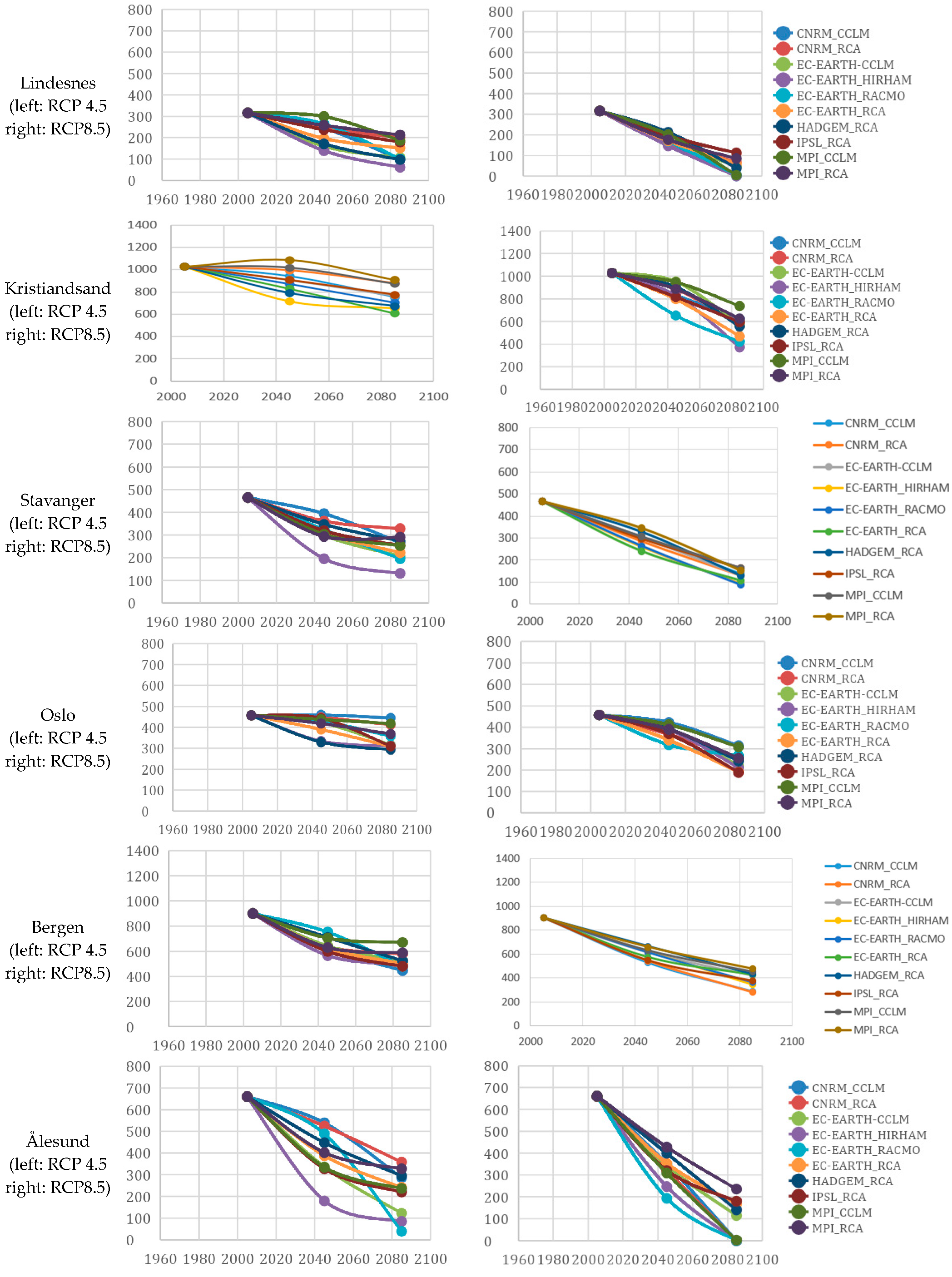
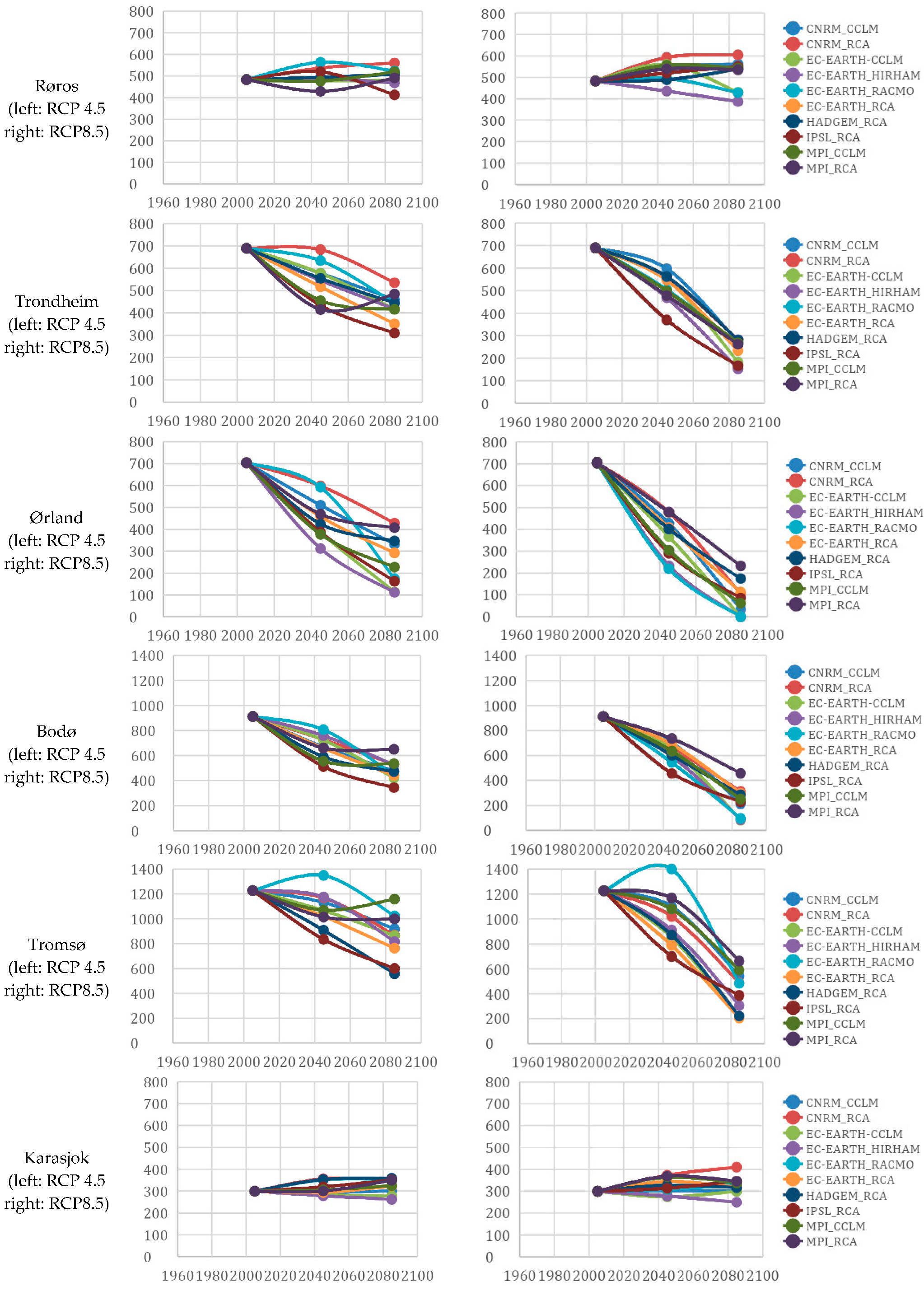
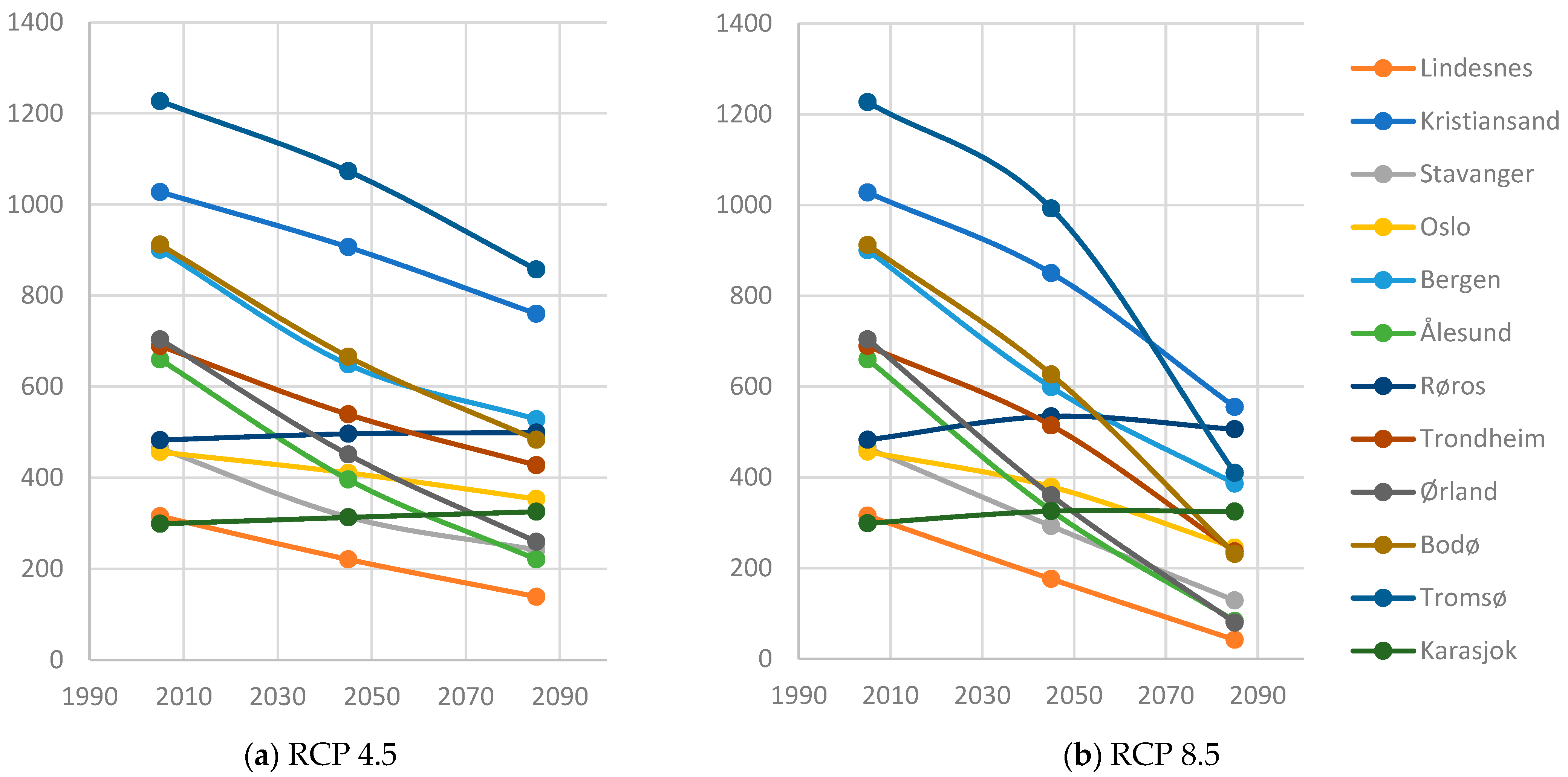
3.3. Estimated Future Development of FDEI Based on Climate Models (2031–2100)

Calculation results for each of the four future scenarios are presented in

Table 5. Future estimated FDEI values for 4-day accumulated rainfall before each frost event for the future period 2031–2060 with emission scenario RCP 4.5.

	Lindesnes	Kristiansand	Stavanger	Oslo	Bergen	Ålesund	Røros	Trondheim	Ørland	Bodø	Tromsø	Karasjok
CNRM_CCLM	244.2	941.4	394.6	459.2	622.6	539.3	484.7	577.9	510.2	667.8	1131.3	292.9
CNRM_RCA	244.5	995.3	361.4	446.9	636.9	524.5	537	683.9	598.4	727.1	1167.6	356.6
EC-EARTH-CCLM	159.8	906.3	297.5	423	641.8	335.6	477	577.6	386.2	723.7	1066.1	282.3
EC-EARTH_HIRHAM	138.8	714.9	195.2	333.5	565.5	179.2	487.5	545.6	312	759.1	1175.1	278.5
EC-EARTH_RACMO	264.5	872	323.8	429.6	753.6	489.1	563.9	634.3	593.1	806.8	1349.2	351.7
EC-EARTH_RCA	195.9	828.8	309.5	389.8	623.9	387.8	500.5	517.1	458.2	658.8	1018.8	293.6
HADGEM_RCA	171.3	789.2	347	329.3	711.3	447.4	494.3	554.4	424.3	589.5	907.7	353.5
IPSL_RCA	237.6	907.7	318.9	443.7	598.8	327	519.7	433.5	386.7	511.7	834.7	319.4
MPI_CCLM	299.3	1019.4	302.9	437.8	705	334.3	476.6	455.2	377.1	555.2	1068.1	305.2
MPI_RCA	257.9	1088.5	293.5	418.5	629.5	401.7	428.6	414.6	469.1	660.4	1013.1	300.2
Average	221	906	314	411	649	397	497	539	452	666	1073	313
Maximum	299	1089	395	459	754	539	564	684	598	807	1349	357
Minimum	139	715	195	329	566	179	429	415	312	512	835	279
Std dev	52	112	53	46	57	109	37	87	94	93	145	30

,

Table 6. Future estimated FDEI values for 4-day accumulated rainfall before each frost event for the future period 2071–2100 with emission scenario RCP 4.5.

	Lindesnes	Kristiansand	Stavanger	Oslo	Bergen	Ålesund	Røros	Trondheim	Ørland	Bodø	Tromsø	Karasjok
CNRM_CCLM	97.4	752.8	266	444.8	446.4	286.2	511.1	459.5	331.7	476.7	918.4	301.9
CNRM_RCA	199.5	880.6	328	412.1	579	358.1	560.4	535.2	428.3	530.4	870.2	354
EC-EARTH-CCLM	106.6	767.9	206.9	316.2	522.3	123	480.9	417.3	113.8	420.5	865.3	278.1
EC-EARTH_HIRHAM	61.3	653	130.6	312.5	495.8	84.8	468.1	417.2	111.5	525.8	817.5	262.2
EC-EARTH_RACMO	100.2	704.8	195.5	357.2	479.5	39.2	523.4	443.9	174.2	441.5	1022.1	353.9
EC-EARTH_RCA	151.7	608.9	221.9	308.2	502.6	241.6	521.3	350.8	292	441.1	763.5	322.8
HADGEM_RCA	96.9	672.4	273.6	293.7	524.6	295.4	506.7	444.9	347	471.5	558.4	358.6
IPSL_RCA	179.2	776.3	254.2	309.4	480.1	220.2	412.7	309.7	162.4	344.3	600.8	351.4
MPI_CCLM	186.9	876.2	253.1	417.9	670.7	237.1	519.5	416	227.4	535.7	1158.5	324.7
MPI_RCA	212.8	910.2	290.7	368.1	587.7	327.8	490.9	484.3	407.5	650.3	998.5	349.5
Average	139	760	242	354	529	221	500	428	260	484	857	326
Maximum	213	910	328	445	671	358	560	535	428	650	1159	359
Minimum	61	609	131	294	446	39	413	310	112	344	558	262
Std dev	53	103	56	55	66	106	40	64	118	83	185	35

,

Table 7. Future estimated FDEI values for 4-day accumulated rainfall before each frost event for the future period 2031–2060 with emission scenario RCP 8.5.

	Lindesnes	Kristiansand	Stavanger	Oslo	Bergen	Ålesund	Røros	Trondheim	Ørland	Bodø	Tromsø	Karasjok
CNRM_CCLM	155.5	830.2	303.9	422.2	525.3	351.1	546.8	597.6	426.6	700.1	1099.6	302.7
CNRM_RCA	162.5	884.3	283.8	366.8	542.3	321.2	593	558.6	477.8	660.5	1020.5	373.5
EC-EARTH-CCLM	169.6	952.9	304.3	392.8	614.1	343.4	560.2	554.1	366.1	650.7	855.4	274.5
EC-EARTH_HIRHAM	147.2	830.1	258.8	389.8	618.9	246.6	436.5	469.2	232.8	595	911.4	277.9
EC-EARTH_RACMO	170.1	651.5	262.9	318.4	612.1	192.8	494.8	504.9	219.4	544.7	1427.8	308.6
EC-EARTH_RCA	171.5	796.5	240.5	340.8	573.9	354.1	607.4	547.2	407	689	789.8	344
HADGEM_RCA	212.9	904.6	327.2	392.6	663.4	399.6	489.2	562.5	400.9	602.5	873.8	327.1
IPSL_RCA	194.9	816.2	295.6	369.4	547.7	321.2	520.7	370.8	290.6	457.1	699	313.1
MPI_CCLM	201.2	947.2	306.6	411.6	628.8	309.2	557	499.6	304	634.7	1079.4	365
MPI_RCA	176.4	886	344.3	389.8	658.3	428.3	539.7	478.7	479	734.6	1168.1	368.8
Average	176	850	293	379	598	327	535	514	360	627	992	326
Maximum	213	953	344	422	663	428	607	598	479	735	1428	374
Minimum	147	652	241	318	525	193	437	371	219	457	699	275
Std dev	21	88	32	31	49	68	51	65	94	81	213	36

and

Table 8. Future estimated FDEI values for 4-day accumulated rainfall before each frost event for the future period 2071–2100 with emission scenario RCP 8.5.

	Lindesnes	Kristiansand	Stav-ager	Oslo	Bergen	Ålesund	Røros	Trondheim	Ørland	Bodø	Tromsø	Karasjok
CNRM_CCLM	0	622.9	138	314.5	285.1	0	561.9	273.5	33.8	214.5	543.4	301
CNRM_RCA	68.4	586	127.9	255.5	281.4	0	605.1	282.6	104.3	312.6	488.7	410
EC-EARTH-CCLM	48.9	566.9	130.5	218.9	422.4	114.5	430.9	183	0	82.6	206.4	299.4
EC-EARTH_HIRHAM	0	372.9	90.2	210.6	343.5	0	387.7	152.9	0	88	306.1	250
EC-EARTH_RACMO	5.7	421.6	86.7	268.1	362.5	0	429.3	264.5	0	97.8	483.5	328.5
EC-EARTH_RCA	61.2	470.3	107.2	190.7	427.8	167.9	481	234.2	112	297.1	205.2	317.5
HADGEM_RCA	38.7	554.7	129.1	241.1	431.7	140.4	538.4	282.4	173.8	286.1	221.6	316
IPSL_RCA	112.7	594.9	162.3	189.3	378.9	180.1	550.8	166.8	84.9	229.2	387	346
MPI_CCLM	4.6	735.4	165.4	307.8	452.2	2.9	543	268.8	61.5	250.8	592.1	336.7
MPI_RCA	85.2	624.9	152.3	256	477	235	535.3	262.2	232.7	458.6	663.4	345.5
Average	43	555	129	245	386	84	506	237	80	232	410	325
Maximum	113	735	165	315	477	235	605	283	233	459	663	410
Minimum	0	373	87	189	281	0	388	153	0	83	205	250
Std dev	40	107	28	44	68	93	70	50	78	119	169	41

for RCP 4.5 (2031–2060), RCP 4.5 (2071–2100), RCP 8.5 (2031–2060) and RCP 8.5 (2071–2100), respectively. The average values and standard deviations were calculated for all locations and scenarios.

The average values from the 10 model chains for each location, timestep and emission scenario are presented in Figure 5 (see graphical presentation of the results from individual model chains in the Appendix A and individual values in Table 5, Table 6, Table 7 and Table 8).

The average FDEI values calculated for the 1991–2020 normal period were higher than the calculated future values for all locations except Røros and Karasjok. These two locations have inland climates characterized by low winter temperatures and precipitation (Figure 1). The most critical future scenario for a given location is difficult to predict beforehand, due to the strong influence of FPC count on the index value as seen by comparing

Table 9. Calculated average FDEI values for historical measurements (1991–2020) and future emission scenarios (RCP 4.5 and RCP 8.5) for time periods 2031–2061 (10 GCM-RCM models) and 2071–2100 (10 GCM-RCM models). The highest value for each location from the five scenarios is highlighted.

	Lindesnes	Kristiansand	Stavanger	Oslo	Bergen	Ålesund	Røros	Trondheim	Ørland	Bodø	Tromsø	Karasjok
1991–2020	316	1027	465	457	900	660	483	690	704	912	1227	299
RCP 4.5 2031–2060	221	906	314	411	649	397	497	539	452	666	1073	313
RCP 4.5 2071–2100	139	760	242	354	529	221	500	428	260	484	857	326
RCP 8.5 2031–2060	176	850	293	379	598	327	535	514	360	627	992	326
RCP 8.5 2071–2100	43	555	129	245	386	84	506	237	80	232	410	325
Max avg value	316	1027	465	457	900	660	535	690	704	912	1227	326

and

Table 10. Calculated average FPC values for historical measurements (1991–2020) and future emission scenarios (RCP 4.5 and RCP 8.5) for time periods 2031–2061 (10 GCM-RCM models) and 2071–2100 (10 GCM-RCM models). The highest value for each location from the five scenarios is highlighted.

	Lindesnes	Kristiansand	Stavanger	Oslo	Bergen	Ålesund	Røros	Trondheim	Ørland	Bodø	Tromsø	Karasjok
1991–2020	30	83	51	76	46	39	115	83	61	72	87	91
RCP 4.5 2031–2060	21	74	40	71	33	25	114	72	45	58	83	99
RCP 4.5 2071–2100	16	65	34	63	27	16	112	62	34	47	74	99
RCP 8.5 2031–2060	19	71	38	68	30	22	115	69	41	55	80	102
RCP 8.5 2071–2100	7	49	22	48	15	5	106	44	19	30	54	99
Max avg value	30	83	51	76	46	39	115	83	61	72	87	102

. Calculating multiple scenarios is therefore essential for the determination of the most conservative scenario, highlighted in the two tables.

3.4. Climate Model Uncertainty Analysis and Design Values of FDEI

To determine the reliability of the index as a design calculation tool, a statistical analysis of the variability in the results is necessary. Three key parameters were selected as indicators: (1) Coefficients of variance (CV) for the FDEI values (

Table 11. Calculated coefficient of variation (normalized standard deviations) for historical measurements (1991–2020) and future emission scenarios (RCP 4.5 and RCP 8.5) for time periods 2031–2060 (10 GCM-RCM models) and 2071–2100 (10 GCM-RCM models). The highest value for each location from the five scenarios is highlighted.

	Lindesnes	Kristiansand	Stavanger	Oslo	Bergen	Ålesund	Røros	Trondheim	Ørland	Bodø	Tromsø	Karasjok
1991–2020	n/a	n/a	n/a	n/a	n/a	n/a	n/a	n/a	n/a	n/a	n/a	n/a
RCP 4.5 2031–2060	0.23	0.12	0.17	0.11	0.09	0.28	0.07	0.16	0.21	0.14	0.14	0.10
RCP 4.5 2071–2100	0.38	0.14	0.23	0.15	0.13	0.48	0.08	0.15	0.45	0.17	0.22	0.11
RCP 8.5 2031–2060	0.12	0.10	0.11	0.08	0.08	0.21	0.10	0.13	0.26	0.13	0.21	0.11
RCP 8.5 2071–2100	0.93	0.19	0.21	0.18	0.18	1.11	0.14	0.21	0.98	0.51	0.41	0.13
Max coeff. of var.	0.93	0.19	0.23	0.18	0.18	1.11	0.14	0.21	0.98	0.51	0.41	0.13

); (2) average FDEI values from the different periods and emission scenarios (Table 9); and (3) the average calculated development trend of the FDEI values (derived from values in Table 9). The suitability of the chosen parameters is further discussed in Section 4.3.

The coefficient of variance for location i, ${CV}_i$, is defined as the normalized standard deviation for location i, as presented in Equation (3).

$${CV}_i={\displaystyle \frac{{SD}_i}{{FDEI}_{i, avg}}}$$

(3)

where ${SD}_i$ is the standard deviation of the model chain output for location i, and ${FDEI}_{i,avg}$ is the average FDEI value for location i, both calculated from the set of 10 different model chains for each timestep and emission scenario given by Table 5, Table 6, Table 7 and Table 8.

Table 12. Normalized range of variance of FDEI for each scenario and location as well as average values for all locations within each scenario.

	Lindesnes	Kristiansand	Stavanger	Oslo	Bergen	Ålesund	Røros	Trondheim	Ørland	Bodø	Tromsø	Karasjok	Average
RCP 4.5 2031–2060	0.36	0.21	0.32	0.16	0.14	0.45	0.14	0.25	0.32	0.22	0.24	0.12	0.24
RCP 4.5 2071–2100	0.54	0.20	0.41	0.21	0.21	0.72	0.15	0.26	0.61	0.32	0.35	0.15	0.34
RCP 8.5 2031–2060	0.19	0.18	0.18	0.14	0.12	0.36	0.16	0.22	0.36	0.22	0.37	0.15	0.22
RCP 8.5 2071–2100	1.32	0.33	0.31	0.26	0.25	1.40	0.21	0.27	1.45	0.81	0.56	0.25	0.62
All scenarios	0.60	0.23	0.30	0.19	0.18	0.73	0.16	0.25	0.68	0.39	0.38	0.17	0.36

and

Table 13. Normalized range of variance of FDEI for each climate model and location as well as average values for all locations per climate model.

	Lindesnes	Kristiansand	Stavanger	Oslo	Bergen	Ålesund	Røros	Trondheim	Ørland	Bodø	Tromsø	Karasjok	Average
CNRM_CCLM	0.98	0.20	0.47	0.18	0.36	0.92	0.07	0.34	0.73	0.47	0.32	0.02	0.42
CNRM_RCA	0.52	0.24	0.42	0.26	0.35	0.87	0.06	0.39	0.61	0.37	0.38	0.07	0.38
EC-EARTH-CCLM	0.50	0.24	0.37	0.30	0.20	0.50	0.13	0.46	0.89	0.68	0.57	0.04	0.41
EC-EARTH_HIRHAM	0.85	0.36	0.50	0.29	0.27	0.97	0.11	0.50	0.95	0.68	0.54	0.05	0.51
EC-EARTH_RACMO	0.96	0.34	0.55	0.24	0.35	1.36	0.13	0.40	1.20	0.75	0.44	0.07	0.57
EC-EARTH_RCA	0.46	0.27	0.46	0.32	0.18	0.38	0.12	0.38	0.55	0.38	0.59	0.08	0.35
HADGEM_RCA	0.67	0.24	0.40	0.24	0.24	0.48	0.05	0.30	0.37	0.32	0.54	0.06	0.33
IPSL_RCA	0.34	0.20	0.30	0.39	0.22	0.28	0.14	0.42	0.65	0.37	0.36	0.06	0.31
MPI_CCLM	0.85	0.16	0.27	0.17	0.21	0.75	0.08	0.28	0.65	0.39	0.29	0.09	0.35
MPI_RCA	0.47	0.26	0.36	0.23	0.15	0.28	0.11	0.27	0.31	0.22	0.26	0.10	0.25
All models	0.66	0.25	0.41	0.26	0.25	0.68	0.10	0.37	0.69	0.46	0.43	0.06	0.39

show the range of variance for the scenarios and the climate models, respectively, relative to the average as per Equation (4).

$${Var}_n=\sum \left(0.5{\displaystyle \frac{X_{n,max}-X_{n,min}}{X_{n,avg}}}\right)$$

(4)

where X_n,max, X_n,min and X_n,avg are the highest, lowest and average index values, respectively, for location n in a given scenario or model.

The proposed design values for FDEI are listed in

Table 14. Design index values. FDEI_d represents the average value from all 10 models for the most critical scenario (see Table 9), CV is the maximum coefficient of variance (see Table 8), and Trend represents model and scenario agreement on expected future development (negative is decreasing FDEI; positive is increasing, and +/− is non-agreement of development between the models and scenarios).

	Lindesnes	Kristiansand	Stavanger	Oslo	Bergen	Ålesund	Røros	Trondheim	Ørland	Bodø	Tromsø	Karasjok
FDEId	316	1027	465	457	900	660	535	690	704	912	1227	326
CV	0.93	0.19	0.23	0.18	0.18	1.11	0.14	0.21	0.98	0.51	0.41	0.13
Trend	+/−	+/−	−	+/−	−	−	+	+/−	−	−	+/−	+

and discussed further in Section 4.3.

4. Discussion

4.1. Historical and Future Developments of FDEI in Norway

As expected, the overall trend for Norway is a decreasing FDEI, which coincides with the results of other studies investigating the risk of frost decay under future climates [50,51,52]. Choidis et al. [51] compared the frost decay risk development of different FPC-based climate indices and a material-based index for a case building in Tønsberg, situated far south-east in Norway, and found an overall decreasing trend. The most similar climates of this data set for comparisons are Kristiansand and Oslo, which display the same decreasing trend. This may be observed both by comparing 1991–2020 results to future scenarios (Figure 5) and by comparing 1991–2020 results to the 1961–1990 results calculated by Lisø et al. [10] (Figure 4). However, the overall declining trend has a few notable exceptions.

Oslo, Karasjok, Røros and Tromsø showed increasing FDEI values between the two historical periods, with the three latter being the coldest three locations of the set. Increased temperatures in these locations resulted in average winter temperatures moving towards 0 °C, while the opposite was true for the other locations.

Looking at the average of the 10 future climate models, a declining trend is found for all locations except Røros and Karasjok, regardless of the emission scenario. Both the mean temperatures and precipitation levels in Norway have increased over the past decades, a trend that is expected to continue in the coming years [53]. An increase in precipitation leads to increased FDEI due to the higher impact of each FPC. However, the development of FPC count in a given location due to increased temperatures depends on whether the climate today is characterized by stable sub-zero temperatures or already fluctuates around 0 °C. This may explain why warm coastal locations in the data set see a reduction in their FDEI values over time, while the opposite is true for cold inland locations (Røros and Karasjok).

Both long timeframes and high-emission scenarios result in declining FDEI for most locations. Even Røros, calculated to have an increasing FDEI for both emission scenarios in the short term as one of the two coldest locations in the set (see Figure 3a) has a declining FDEI from 2031–2060 to 2071–2100 under RCP 8.5 (Table 9). Because warmer winters lead to fewer FPCs in Røros (Table 10), the FDEI is reduced. Therefore, the risk of frost decay of brick facades is a declining problem for locations with high present-day FDEI in Norway but an intensifying problem for cold locations in the short term.

4.2. Uncertainties Originating from Future Climate Projections

FPCs derived from the climate data, both historical measurements and future climate scenarios, are derived from daily max/min values in the models. The choice of temporal resolution is a tradeoff between model quality and quantity. The coarse temporal resolution selected here substitutes the precision of hourly data for a large quantity of climate models, emission scenarios and locations. Thus, the index may be easily expanded by increasing the spatial resolution. Importantly, it also enables a comprehensive assessment of the scenario-induced uncertainties in the results by analyzing inter-model variations, scenario differences and temporal developments.

The complexity of this index increases the uncertainty of future estimations, compared to more directly derived climate indices, such as the Scheffer index [54], or FPC-based indices [51,55]. Future estimations of FDEI show higher uncertainty than future estimations of the Scheffer index, which is an expression of average monthly temperatures and precipitation levels [54], also calculated for the Norwegian 1961–1990 climate normal by Lisø et al. [56]. The Scheffer index is more reliant on climate than weather, using monthly average values for temperature and accumulated precipitation, while the frost index is derived from daily accumulated weather events. It depends on the co-occurrence of precipitation events and FPCs, neither of which can be derived from average values. The same principle holds when comparing uncertainties in FPC-based climate indices and FDEI-based climate indices, as the latter is a combination of freezing-point crossings and precipitation events. This may explain the high variation in future model outputs as well as the sensitivity of the index to methodological choices, such as the temporal resolution of the model.

For all locations except Stavanger, the RCP 8.5 emission scenario in 2071–2100 had the highest CV, indicating that the most extreme scenario and longest timeframe yielded the highest uncertainties. The same trend occurred when comparing RCP 4.5 results for 2031–2060 and 2071–2100; thus, longer timeframes increase the variance between the model chains, regardless of emission scenario forcing.

A comparison of the GCM and scenario uncertainties conducted by Shen et al. revealed that differences in temperature predictions are larger between scenarios than among different climate models for the 2071–2100 climate [23]. Furthermore, Hawkins and Sutton concluded that model uncertainty is the dominant source of uncertainty in precipitation predictions, finding significant variability between models [47]. Such findings, pointing to the necessity of considering an ensemble of climate models, are frequently found in the literature, especially when precipitation predictions exert significant influence on the final results [23,51,57,58]. However, the temporal scale of the model has an influence on the relative distribution of uncertainties, suggesting that scenario uncertainties generally have larger impacts on the results in the long term, while internal model variation and inter-model variability has a larger impact in the short term [11]. These findings are also evident from the analysis of variance in temperature and precipitation from different scenarios and models used as an input in this study, illustrated in Figure 3.

However, for the FDEI derived from the climate parameters, the conclusions were less clear. The range of variance for RCP 4.5 in the 2071–2100 period was 34% when averaging all locations, whereas the same variable for RCP 8.5 was 62%. The range of variance for the different models within all scenarios was between 25 and 57%, with an average of 39% for all models and locations. Hence, scenario uncertainty and climate model uncertainty were within a similar range for the FDEI. This result is logical, as predicting FDEI values based on climate parameter predictions is more complex than predicting climate parameters. Predicting precipitation in co-occurrence with temperature changes is more uncertain than predicting precipitation alone, thereby increasing the uncertainty of the output (expressed here as the variance between models). This is in line with similar studies analyzing sources of uncertainty in future climate models [50,59,60], highlighting the importance of considering multiple scenarios and climate models to treat uncertainties adequately.

4.3. FDEI as a Design Tool in Building Design

In order for the index to be useful as a design tool in moisture safety design, the values must be conservative. A frequently used method for estimating conservative design values is to calculate the 95% confidence interval. Using FDEI values with a 95% confidence interval would give more conservative values for locations with high coefficients of variance, thus accounting for climate model uncertainties. However, this is problematic for locations where all model chains agree that the FDEI will decrease in all future scenarios but disagree on the rate of decrease. Because they disagree on how fast the decrease occurs, the variability is so high that the maximum 95% confidence interval suggests an increase in future FDEI values. This trend was observed in 5 of the 12 locations (Table 14). The reason for this high variance is the complexity of the index. The estimated annual sum of accumulated precipitation in the 4 days before each freezing event requires predicting the co-occurrence of two parameters with variance between models. As the high uncertainty in the results would overshadow the overall trend, the conclusion is to divide the results into the best estimated value (average), an expression of variation (CV) and an overall trend (increasing, decreasing, stable). This makes it more challenging to use the index as it is less “pre-analyzed”, but users have more information to make risk assessments with three values rather than one. The CV is preferred over the simpler expression of standard deviation because the former expresses the uncertainty relative to the index value, making it more suitable as a comparative expression of uncertainty across FDEI values.

Earlier studies have highlighted the need for quick-to-use qualitative tools for climate adaptation in building moisture design, such as comparative risk analysis and qualitative robustness assessments [14]. For the index to be applicable as a design tool, it should (1) describe a relevant climate stress, (2) be relatively differentiated between locations, enabling comparative evaluations, and (3) have absolute values that are correlated with material response, enabling design recommendations [9].

Here, the first premise is valid because frost decay is among the most important degradation factors for brick facades in Norway [31]. Grossi et al. concludes that using an FPC index to predict frost decay risks may be sufficient, as FPCs display the same features as the more complex FDEI [55]. This is, however, countered by other studies, arguing that using FPC directly will overestimate the risk due to simplifications of the precipitation influence on the results [51]. Comparing the development of the calculated FDEI and FPC in this study (Table 9 and Table 10), the conclusion by Grossi et al. is correct when considering each location in isolation. However, by comparing the values in the location set relative to each other (Table 9 and Table 10), FDEI and FPC are not in agreement as to which location has the highest risk of frost decay. Røros and Karasjok (the two coldest and dryest locations) have the two highest FPC values in the set (115 and 91, respectively, for 1991–2020), but both have moderate to low FDEI values (483 and 299, respectively), suggesting that FPC values underestimate the influence of precipitation in the given climate.

The second premise, relative differentiation between locations, is also valid as variance in climate, both temperature and precipitation, is high in the data set, enabling comparative risk evaluations between locations.

The connection between the FDEI and material response (premise 3) is outside the scope of this study but could be investigated through the development of response-based indices using HAM-software, as discussed in Section 4.4. Lacking this comparison, the design engineer considering a building in a given location relies on a qualitative evaluation of the given FDEI value relative to known high and low risks from the data set, as well as considerations of FDEI future development trends for the location (see Table 14).

4.4. Limitations and Scope for Further Research

Climate indices such as the FDEI require response correlation to be useful as design tools, either by comparing values to known high-risk locations or by comparing values to known high-risk absolute values for a given material or solution. For the latter analysis to be possible, threshold values dependent on material parameters must be identified. Following the methodology developed by, e.g., Vandemeulebroucke [30] or Choidis [51], comparison to response-based indices using HAM-software could be investigated. Pairing material responses to FDEI values for a selection of climates may thus enable direct design recommendations based on the absolute quantified FDEI values for a given location. Material responses to different FDEI benchmarks may also be investigated through systematic laboratory experiments and correlated with in situ performance through field investigations.

All three methods for correlating material responses to index values require wind loads to be considered. Such as it is, the FDEI expresses the climatic potential for frost decay at a given location rather than the actual climate load. Wind-driven rain effects should therefore be considered as possible further developments of the FDEI, as also pointed out by Lisø et al. [10]. However, this may complicate the FDEI to such an extent that its usefulness in moisture safety design is compromised. If so, a separate evaluation of driving rain exposure may be a good option, which could be coupled with the FDEI through an overall risk assessment for robustness [35].

The original index values for 1961–1990 calculated by Lisø et al. [10] are lower than those calculated here owing to a methodology bias in the model’s temporal resolution. As shown in Table 3, when calculating the FDEI using daily max/min values of temperature instead of temperatures at synoptic times, the index value was 2.1 times higher on average (±0.3, 95% conf int). Because of this sensitivity, correlating the absolute index values to material responses with sufficient certainty may prove difficult, as concluded by other studies on frost resistance in clay bricks [61]. Further studies on how the FDEI can be implemented in moisture safety design should, therefore, investigate methods for evaluating the risk of frost decay for a given index value.

5. Conclusions

The following conclusions may be made based on the result analysis:

• The development of FDEI values in Norway over the last decades have declined when comparing climate data from 1961–1990 to 1991–2020, due to increasing winter temperatures from climate changes. Notable exceptions to the trend are found in the coldest locations (Røros, Karasjok, Tromsø, Oslo), where the net effect of increased winter temperatures and increased precipitation leads to an increase in FDEI values. In the future, the overall reduction in FDEI values is expected to continue for all locations except Røros and Karasjok, where annual freezing-point crossings are relatively stable even when considering the RCP 8.5 2071–2100 scenario, leading to an increase in FDEI values.
• Additional uncertainties in the calculation of FDEI values are introduced when using future climate projections. A comparison of the 10 climate models revealed significant variations, demonstrating that introducing future estimates increases the level of uncertainty in such calculations. In particular, the results show that longer timeframes increase the variance between the model chains, independent of emission scenario forcing, and more extreme emission scenario forcings further increase the variance. Therefore, assessments of future climate scenarios should be calculated using an ensemble of models and emission scenarios to assess the uncertainty of the results.
• For the index to be useful as a design tool, design values and information describing design value uncertainty must be defined. The proposed design value for each location is conservatively defined as the highest average FDEI value in the data set for each location (either from the 1991–2020 period or from one of the four future scenarios). The coefficient of variance, CV, for each design value calculation is defined, as well as the estimated future development trend for the location. A comparison of the index value for the given location relative to other locations in the set indicates whether the location is a high- or low-risk area for frost decay, and evaluating CV and development trends allows for an uncertainty analysis of the conclusion. This approach enables a quick-to-use qualitative comparative risk analysis for climate adaptation purposes, in line with the climate risk and vulnerability assessment required in the EU Taxonomy Regulation.

References

1. Grynning, S.; Wærnes, E.; Kvande, T.; Time, B. Climate adaptation of buildings through MOM-and upgrading-State of the art and research needs. Energy Procedia 2017, 132, 622–627. [Google Scholar] [CrossRef]
2. Häkkinen, T.; Belloni, K. Barriers and drivers for sustainable building. Build. Res. Inf. 2011, 39, 239–255. [Google Scholar] [CrossRef]
3. Singh, C.; Iyer, S.; New, M.G.; Few, R.; Kuchimanchi, B.; Segnon, A.C.; Morchain, D. Interrogating ‘effectiveness’ in climate change adaptation: 11 guiding principles for adaptation research and practice. Clim. Dev. 2022, 14, 650–664. [Google Scholar] [CrossRef]
4. Lisø, K.R.; Kvande, T.; Time, B. climate adaptation framework for moisture-resilient buildings in Norway. Energy Procedia 2017, 132, 628–633. [Google Scholar] [CrossRef]
5. Bunkholt, N.S.; Gullbrekken, L.; Time, B.; Kvande, T. Process induced building defects in Norway—Development and climate risks. J. Phys. Conf. Ser. 2021, 2069, 012040. [Google Scholar] [CrossRef]
6. Rydock, J.P.; Lisø, K.R.; Førland, E.J.; Nore, K.; Thue, J.V. A driving rain exposure index for Norway. Build. Environ. 2005, 40, 1450–1458. [Google Scholar] [CrossRef]
7. Pakkala, T.A.; Lahdensivu, J. Wind-driven rain load in Finland in present and future projected climates. J. Phys. Conf. Ser. 2023, 2654, 012012. [Google Scholar] [CrossRef]
8. Gaur, A.; Lu, H.; Lacasse, M.; Ge, H.; Hill, F. Future projected changes in moisture index over Canada. Build. Environ. 2021, 199, 107923. [Google Scholar] [CrossRef]
9. Gaarder, J.E.; Andenæs, E.; Astrup, I.; Lacasse, M.; Time, B.; Kvande, T. Comparing Canadian and Norwegian moisture indices for building climate adaptation. J. Phys. Conf. Ser. 2023, 2654, 012013. [Google Scholar] [CrossRef]
10. Lisø, K.R.; Kvande, T.; Hygen, H.O.; Thue, J.V.; Harstveit, K. A frost decay exposure index for porous, mineral building materials. Build. Environ. 2007, 42, 3547–3555. [Google Scholar] [CrossRef]
11. Lehner, F.; Deser, C.; Maher, N.; Marotzke, J.; Fischer, E.M.; Brunner, L.; Knutti, R.; Hawkins, E. Partitioning climate projection uncertainty with multiple large ensembles and CMIP5/6. Earth Syst. Dyn. 2020, 11, 491–508. [Google Scholar] [CrossRef]
12. Sahlin, U.; Helle, I.; Perepolkin, D. “This Is What We Don’t Know”: Treating Epistemic Uncertainty in Bayesian Networks for Risk Assessment. Integr. Environ. Assess. Manag. 2021, 17, 221–232. [Google Scholar] [CrossRef] [PubMed]
13. Gaarder, J.E.; Hygen, H.O.; Bohne, R.A.; Kvande, T. Building Adaptation Measures Using Future Climate Scenarios—A Scoping Review of Uncertainty Treatment and Communication. Buildings 2023, 13, 1460. [Google Scholar] [CrossRef]
14. Gaarder, J.E.; Høien Clausen, R.; Næss, R.; Kvande, T. Barriers to Climate Adaptation in Norwegian Building Projects–Insights from Moisture Safety Designers’ Perspective. Clim. Risk Manag. 2024, 43, 100590. [Google Scholar] [CrossRef]
15. Kvande, T.; Tajet, H.T.T.; Tunheim, K. Klimadata for dimensjonering mot regnpåkjenning. In SINTEF, Building Research Design Guides; SINTEF AS: Oslo, Norway, 2023; Available online: https://www.byggforsk.no/sok/2?sources=1&source=1&q=Klimadata+for+dimensjonering+mot+regnp%C3%A5kjenning (accessed on 4 September 2024).
16. Kvande, T.; Tajet, H.T.T.; Hygen, H.O. Klimadata for termisk dimensjonering og frostsikring. In SINTEF, Building Research Design Guides; SINTEF AS: Oslo, Norway, 2023; Available online: https://www.byggforsk.no/sok/2?sources=1&source=1&q=Klimadata+for+termisk+dimensjonering+og+frostsikring (accessed on 4 September 2024).
17. WMO. Guidelines on analysis of extremes in a changing climate in support of informed decisions for adaptation. World Meteorol. Organ. 2009, 1500, 72. [Google Scholar]
18. Tveito, O.E. Norwegian Standard Climate Normals; Norwegian Meteorological Institute: Oslo, Norway, 2021. [Google Scholar]
19. Hanssen-Bauer, I.; Tveito, O.E.; Tajet, H.T.T.; Skaland, R.G. Temperatur- og Nedbør-Regioner i Norge; Norwegian Meteorological Institute: Oslo, Norway, 2022. [Google Scholar]
20. Berkhout, F.; Hertin, J.; Gann, D.M. Learning to adapt: Organisational adaptation to climate change impacts. Clim. Chang. 2006, 78, 135–156. [Google Scholar] [CrossRef]
21. Bevan, L.D. The ambiguities of uncertainty: A review of uncertainty frameworks relevant to the assessment of environmental change. Futures 2022, 137, 102919. [Google Scholar] [CrossRef]
22. Manning, M.; Lawrence, J.; King, D.N.; Chapman, R. Dealing with changing risks: A New Zealand perspective on climate change adaptation. Reg. Environ. Chang. 2015, 15, 581–594. [Google Scholar] [CrossRef]
23. Shen, M.; Chen, J.; Zhuan, M.; Chen, H.; Xu, C.-Y.; Xiong, L. Estimating uncertainty and its temporal variation related to global climate models in quantifying climate change impacts on hydrology. J. Hydrol. 2018, 556, 10–24. [Google Scholar] [CrossRef]
24. Opoku, D.-G.J.; Ayarkwa, J.; Agyekum, K. Barriers to environmental sustainability of construction projects. Smart Sustain. Built Environ. 2019, 8, 292–306. [Google Scholar] [CrossRef]
25. Simonet, G.; Leseur, A. Barriers and drivers to adaptation to climate change—A field study of ten French local authorities. Clim. Chang. 2019, 155, 621–637. [Google Scholar] [CrossRef]
26. Haarhaus, T.; Liening, A. Building dynamic capabilities to cope with environmental uncertainty: The role of strategic foresight. Technol. Forecast. Soc. Chang. 2020, 155, 120033. [Google Scholar] [CrossRef]
27. Stanton, M.C.B.; Roelich, K. Decision making under deep uncertainties: A review of the applicability of methods in practice. Technol. Forecast. Soc. Chang. 2021, 171, 120939. [Google Scholar] [CrossRef]
28. Clarke, D.; Murphy, C.; Lorenzoni, I. Barriers to Transformative Adaptation: Responses to Flood Risk in Ireland. J. Extreme Events 2016, 3, 1650010. [Google Scholar] [CrossRef]
29. Ryan, B.; Bristow, D.N. Climate Change and Hygrothermal Performance of Building Envelopes: A Review on Risk Assessment. Int. J. Technol. 2023, 14, 1461–1475. [Google Scholar] [CrossRef]
30. Vandemeulebroucke, I.; Kotova, L.; Caluwaerts, S.; Van Den Bossche, N. Degradation of brick masonry walls in Europe and the Mediterranean: Advantages of a response-based analysis to study climate change. Build. Environ. 2023, 230, 109963. [Google Scholar] [CrossRef]
31. Kvande, T.; Lisø, K.R. Climate adapted design of masonry structures. Build. Environ. 2009, 44, 2442–2450. [Google Scholar] [CrossRef]
32. Ojo, B. Strategies for the Optimization of Critical Infrastructure Projects to Enhance Urban Resilience to Climate Change. J. Sci. Eng. Res. 2024, 11, 107–123. [Google Scholar]
33. EU. Regulation (EU) 2020/852 of the European Parliament and of the Council of 18 June 2020 on the establishment of a framework to facilitate sustainable investment, and amending Regulation (EU) 2019/2088. Off. J. Eur. Union 2020, 198, 13–43. [Google Scholar]
34. Janssens, K.; Marincioni, V.; Van Den Bossche, N. Improving hygrothermal risk assessment tools for brick walls in a changing climate. J. Phys. Conf. Ser. 2023, 2654, 012024. [Google Scholar] [CrossRef]
35. Pakkala, T.A.; Köliö, A.; Lahdensivu, J.; Kiviste, M. Durability demands related to frost attack for Finnish concrete buildings in changing climate. Build. Environ. 2014, 82, 27–41. [Google Scholar] [CrossRef]
36. Mandinec, J.; Johansson, P. Microclimate modelling and hygrothermal investigation of freeze-thaw degradation under future climate scenarios. J. Phys. Conf. Ser. 2023, 2654, 012146. [Google Scholar] [CrossRef]
37. Köppen, W. Das geographische System der Klimate. In Handbuch der Klimatologie, s. 46; Borntraeger: Stuttgart, Germany, 1936. [Google Scholar] [CrossRef]
38. MET. Norwegian Meteorological Institute. 2024. Available online: https://www.seklima.met.no (accessed on 1 April 2024).
39. Venter, Z.S.; Krog, N.H.; Barton, D.N. Linking green infrastructure to urban heat and human health risk mitigation in Oslo, Norway. Sci. Total Environ. 2020, 709, 136193. [Google Scholar] [CrossRef] [PubMed]
40. Lussana, C. seNorge observational gridded datasets. seNorge_2018, version 20.05. arXiv 2020, arXiv:2008.02021. [Google Scholar]
41. Lussana, C.; Tveito, O.E.; Dobler, A.; Tunheim, K. seNorge_2018, daily precipitation, and temperature datasets over Norway. Earth Syst. Sci. Data 2019, 11, 1531–1551. [Google Scholar] [CrossRef]
42. Wong, W.K.; Nilsen, I.B. Bias-Adjustment of Maximum and Minimum Temperatures for Norway; Norwegian Water Resources and Energy Directorate: Oslo, Norway, 2019. [Google Scholar]
43. Wong, W.K.; Haddeland, I.; Lawrence, D.; Beldring, S. Gridded 1 × 1 km Climate and Hydrological Projections for Norway; Norwegian Water Resources and Energy Directorate: Oslo, Norway, 2016. [Google Scholar]
44. Jacob, D.; Petersen, J.; Eggert, B.; Alias, A.; Christensen, O.B.; Bouwer, L.M.; Braun, A.; Colette, A.; Déqué, M.; Georgievski, G. EURO-CORDEX: New high-resolution climate change projections for European impact research. Reg. Environ. Chang. 2014, 14, 563–578. [Google Scholar] [CrossRef]
45. Stocker, T.F.; Qin, D.; Plattner, G.-K.; Tignor, M.M.; Allen, S.K.; Boschung, J.; Nauels, A.; Xia, Y.; Bex, V.; Midgley, P.M. Climate Change 2013: The Physical Science Basis. Contribution of Working Group I to the Fifth Assessment Report of IPCC the Intergovernmental Panel on Climate Change; Cambridge University Press: Cambridge, UK, 2014. [Google Scholar] [CrossRef]
46. Giorgi, F.; Mearns, L.O. Introduction to special section: Regional Climate Modeling Revisited. J. Geophys. Res. Atmos. 1999, 104, 6335–6352. [Google Scholar] [CrossRef]
47. Hawkins, E.; Sutton, R. The potential to narrow uncertainty in projections of regional precipitation change. Clim. Dyn. 2011, 37, 407–418. [Google Scholar] [CrossRef]
48. Martel, J.-L.; Brissette, F.P.; Lucas-Picher, P.; Troin, M.; Arsenault, R. Climate Change and Rainfall Intensity–Duration–Frequency Curves: Overview of Science and Guidelines for Adaptation. J. Hydrol. Eng. 2021, 26, 03121001. [Google Scholar] [CrossRef]
49. Fischer, E.M.; Sedláček, J.; Hawkins, E.; Knutti, R. Models agree on forced response pattern of precipitation and temperature extremes. Geophys. Res. Lett. 2014, 41, 8554–8562. [Google Scholar] [CrossRef]
50. Vandemeulebroucke, I.; Caluwaerts, S.; Van Den Bossche, N. Factorial Study on the Impact of Climate Change on Freeze-Thaw Damage, Mould Growth and Wood Decay in Solid Masonry Walls in Brussels. Buildings 2021, 11, 134. [Google Scholar] [CrossRef]
51. Choidis, P.; Coelho, G.B.A.; Kraniotis, D. Assessment of frost damage risk in a historic masonry wall due to climate change. Adv. Geosci. 2023, 58, 157–175. [Google Scholar] [CrossRef]
52. Loli, A.; Bertolin, C. Indoor Multi-Risk Scenarios of Climate Change Effects on Building Materials in Scandinavian Countries. Geosciences 2018, 8, 347. [Google Scholar] [CrossRef]
53. Hanssen-Bauer, I.; Drange, H.; Førland, E.J.; Roald, L.A.; Børsheim, K.Y.; Hisdal, H.; Lawrence, D.; Nesje, A.; Sandven, S.; Sorteberg, A. Climate in Norway 2100. In Background Information to NOU Climate Adaptation (In Norwegian: Klima i Norge 2100. Bakgrunnsmateriale til NOU Klimatilplassing); Norsk klimasenter: Oslo, Norway, 2017. [Google Scholar]
54. Scheffer, T.C. A climate index for estimating potential for decay in wood structures above ground. For. Prod. J. 1971, 21, 25–31. [Google Scholar]
55. Grossi, C.M.; Brimblecombe, P.; Harris, I. Predicting long term freeze–thaw risks on Europe built heritage and archaeological sites in a changing climate. Sci. Total Environ. 2007, 377, 273–281. [Google Scholar] [CrossRef]
56. Lisø, K.R.; Hygen, H.O.; Kvande, T.; Thue, J.V. Decay potential in wood structures using climate data. Build. Res. Inf. 2006, 34, 546–551. [Google Scholar] [CrossRef]
57. Gaur, A.; Lacasse, M.; Armstrong, M. Climate Data to Undertake Hygrothermal and Whole Building Simulations Under Projected Climate Change Influences for 11 Canadian Cities. Data 2019, 4, 72. [Google Scholar] [CrossRef]
58. Smith, D.M.; Scaife, A.A.; Eade, R.; Athanasiadis, P.; Bellucci, A.; Bethke, I.; Bilbao, R.; Borchert, L.F.; Caron, L.-P.; Counillon, F.; et al. North Atlantic climate far more predictable than models imply. Nature 2020, 583, 796–800. [Google Scholar] [CrossRef]
59. Jeong, D.I.; Cannon, A.J. Projected changes to moisture loads for design and management of building exteriors over Canada. Build. Environ. 2020, 170, 106609. [Google Scholar] [CrossRef]
60. Dukhan, T.; Sushama, L. Understanding and modelling future wind-driven rain loads on building envelopes for Canada. Build. Environ. 2021, 196, 107800. [Google Scholar] [CrossRef]
61. Calle, K.; Van Den Bossche, N. Analysis of Different Frost Indexes and Their Potential to Assess Frost Based on HAM Simulations. In Proceedings of the 14th International Conference on Durability of Buildings Materials and Components, Ghent, Belgium, 29–31 May 2017; RILEM Publications SARL: Paris, France, 2017; pp. 61–62. Available online: http://hdl.handle.net/1854/LU-8525026 (accessed on 4 September 2024).
Figure 1. Maps for the 1991–2020 normal period. (a) Climate classification according to the Köppen-Geiger system; (b) Annual precipitation; (c) Annual average temperature.
Buildings 14 02873 g001
Figure 2. Visual representation of the calculation model, illustrating the connection between historical measurement data, climate models, future scenarios and FDEI calculations.
Buildings 14 02873 g002
Figure 5. Calculated evolution of average FDEI values for each location and timestep (1991–2020, 2031–2061, 2071–2100). The period 1991–2020 is based on historical measurements, given by Table 3, and future periods are based on climate model outputs, given by Table 5, Table 6, Table 7 and Table 8.
Buildings 14 02873 g005