Stochastic Response of Composite Post Insulators under Seismic Excitation

Abstract

Composite post insulators are crucial facilities in substations and are prone to significant damage during seismic disasters. However, existing research lacks seismic motion models suitable for power facilities and rarely involves stochastic models. Furthermore, considering the non-stationary characteristics of seismic motion, predicting the response of nonlinear systems under non-stationary excitation becomes exceedingly challenging. In view of this, the stochastic response of composite post insulators under the non-stationary stochastic seismic excitation appropriate for power facilities has been studied. First, a stochastic ground motion model, conforming to the Code for Seismic Design of Electrical Insulators in China, is established, incorporating amplitude and frequency non-stationarity. Next, the nonlinear dynamic system, accounting for multi-section composite post insulators and the nonlinearity of flange connections, is established under stochastic ground motion conditions. Based on this stochastic nonlinear dynamic model, the dynamic behavior of the system was analyzed using the stochastic dynamics method (the wavelet-Galerkin method), and the influence of nonlinear stiffness on the system response was discussed. The stochastic seismic response analysis method proposed in this paper can serve as a valuable reference for the seismic design of pillar-type electrical equipment.

1. Introduction

Seismic motion poses significant threats to various structures, including high-rise buildings [1], bridges [2] and electrical facilities in substations [3]. Historical earthquakes in China have caused severe damage to electrical equipment, particularly pillar electrical equipment in substations [4]. Experimental findings from shaking table tests on composite post insulators indicate that high-voltage electrical equipment displays significant nonlinear characteristics when exposed to seismic wave stimulation [5]. These nonlinear characteristics primarily stem from the inherent structural features of the pillar equipment and the varied material compositions of the flange mounting elements within their constituent parts. Nevertheless, previous studies on the dynamics of pillar electrical equipment under earthquakes barely accounted for nonlinear factors, with analysis methods mostly relying on numerical simulations, thereby limiting the accuracy of seismic capacity assessments of substations.

Currently, significant advancements have been achieved in the study of ground motion models. Numerous researchers have developed power spectral density function models for ground motion accelerations using actual earthquake acceleration records. The most common model is the Kanai–Tajimi spectrum [6]. Several researchers have proposed enhanced models based on this foundation, including the Clough–Penzien modified double-filtered white noise model [7], OU’s filtered white noise model [8], and Liu’s probabilistic model of completely non-stationary ground motion processes [9]. In practical scenarios, the seismic power spectrum varies significantly due to diverse environments and excitation sources. For example, Erhan et al. [10] specially analyzed the characteristics of ground motion response in Turkey. Nevertheless, existing research lacks a stochastic model and parameters that can be applied to the seismic analysis of power facilities in China.

This paper investigates the nonlinear dynamic response of multi-section composite post insulators to stochastic ground motion. Initially, we establish the probability model for the completely non-stationary ground motion process and determine the model parameters according to the current “Code for Seismic Design of Electrical Installations” [11] in China. Next, we transform the nonlinear dynamic differential equation into a set of nonlinear algebraic equations and the harmonic wavelet basis functions using the Galerkin method [12]. Subsequently, we solve this set of algebraic equations, which express the relationship between the input wavelet transform and the nonlinear output wavelet transform, using the Newton iteration method. Lastly, we obtain the dynamic response of the nonlinear oscillator under ground motion excitation.

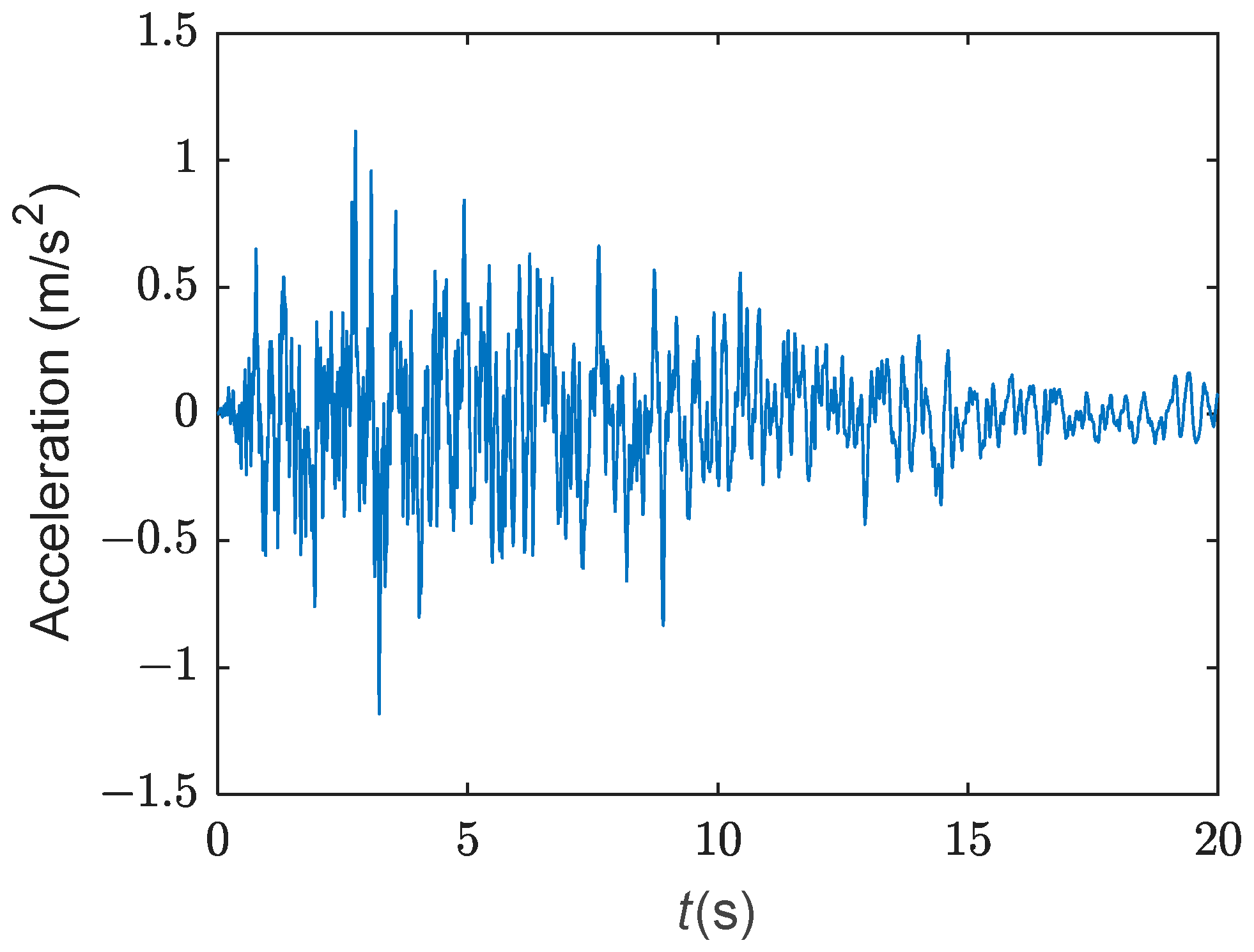
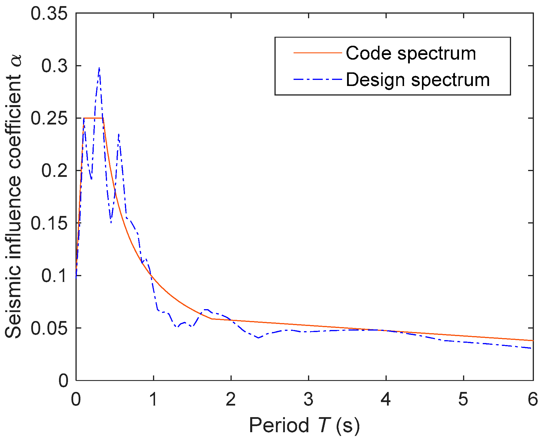
2. Stochastic Ground Motion Model

In the nonlinear seismic analysis of intricate engineering structures, deterministic structural dynamic analysis typically involves selecting several seismic motion records or artificial seismic motion time histories [13]. However, deterministic methods fail to fully capture the randomness of seismic motion and the extensive probability information regarding structural seismic response. Employing stochastic seismic motion models can address this issue by providing high-order statistics or probability density functions of structural response for subsequent analyses, such as structural reliability assessments [14].

In prior research, the majority of stochastic seismic motion models have focused on stationary models due to their simpler theoretical analysis compared to non-stationary scenarios [15]. Nonetheless, notable disparities exist in the time-domain statistical features between stationary random seismic motion models and actual seismic motion records. Consequently, researchers have shifted their focus to developing amplitude non-stationary models, placing greater emphasis on the influence of non-stationary characteristics of seismic intensity on the random seismic response of structures [16]. Recent studies, however, have increasingly shown that both amplitude and frequency non-stationarity substantially impact the mechanical behavior of structures, particularly as they enter the nonlinear stage [17,18]. Therefore, this paper addresses the most general case that both the amplitude and frequency of the ground motion process are non-stationary.

The real non-stationary process simulated from the spectrum can be expressed as follows [10]:

$$f(t)={\displaystyle \sum _{n=1}^N\sqrt{2G_U\left(t,{\omega }_n\right)\Delta \omega }}\left[\cos \left({\omega }_{n}t\right)X_n+\sin \left({\omega }_{n}t\right)Y_n\right]$$

(1)

where f(t) is a simulated non-stationary process, ${\omega }_n=n\Delta \omega$. The frequency interval $\Delta \omega$ needs to be small enough to meet the accuracy requirements. $X_n$ and $Y_n$(n = 1, 2, …, N) are standard orthogonal random variables, which can be taken as

$$\begin{array}{l}{\overline{X}}_k=\sqrt{2}\cos (k\mathsf{\Theta }+\pi /4),{\overline{Y}}_k=\sqrt{2}\sin (k\mathsf{\Theta }+\pi /4),\\ k=1,2,\cdots ,N\end{array}$$

(2)

where random variable $\mathsf{\Theta }$ is uniformly distributed on the interval [−π,π].

The evolutionary power spectrum of non-stationary processes $G_U\left(t,{\omega }_n\right)$ in Equation (1) can be expressed as

$$G_U(t,\omega )=|A(t,\omega ){|}^{2}G(\omega )$$

(3)

where $G_U(t,\omega )$ is the unilateral evolutionary power spectrum; $G(\omega )$ is the unilateral power spectrum of the acceleration process of stationary ground motion. The non-stationary amplitude and frequency of this stochastic seismic motion model are reflected by the time–frequency modulation function $A(t,\omega )$ in Equation (3), which is based on the amplitude modulation function [16]. And the expression of the function $A(t,\omega )$ is

$$A(t,\omega )=\frac{\exp (-a\times t)-\exp \left[-\left(c\left|\omega -{\omega }_{\mathrm{g}}\right|+b\right)\times t\right]}{\exp \left(-a\times t^{*}\right)-\exp \left[-\left(c\left|\omega -{\omega }_{\mathrm{g}}\right|+b\right)\times t^{*}\right]},\omega >0,\hspace{1em}t>0$$

(4)

where

$$\begin{array}{l}{t}^{*}=\frac{\ln \left(c\times \left|\omega -{\omega }_{\mathrm{g}}\right|+b\right)-\ln (a)}{c\times \left|\omega -{\omega }_{\mathrm{g}}\right|+(b-a)};\\ b=a+0.001,c=0.005,\omega >0\end{array}$$

(5)

The value a is determined by site factors.

For the power spectrum of a stationary process $G(\omega )$, use the Clough–Penzien spectrum [8]:

$$G(\omega )=2S(\omega )=2\times \frac{{\omega }_{\mathrm{g}}^4+4{\xi }_{\mathrm{g}}^2{\omega }_{\mathrm{g}}^2{\omega }^2}{{\left({\omega }^2-{\omega }_{\mathrm{g}}^2\right)}^2+4{\xi }_{\mathrm{g}}^2{\omega }_{\mathrm{g}}^2{\omega }^2}\times \frac{{\omega }^4}{{\left({\omega }^2-{\omega }_{\mathrm{f}}^2\right)}^2+4{\xi }_{\mathrm{f}}^2{\omega }_{\mathrm{f}}^2{\omega }^2}{S}_0,\omega >0$$

(6)

where ${\omega }_{\mathrm{g}}$ and ${\xi }_{\mathrm{g}}$ denote the dominant frequency and damping ratio of site soil, respectively; ${\omega }_{\mathrm{f}}$ and ${\xi }_{\mathrm{f}}$ denote the parameters of the filter hindering the low-frequency components of seismic acceleration; and $S_0$ is the spectral intensity factor.

The proper selection of model parameters is crucial for analyzing stochastic responses when employing the stochastic ground motion model. This paper focuses on composite post insulators used in electrical installations and we select common sites of power facilities as representative parameters in accordance with GB50260-2013. Thus, considering a seismic fortification intensity of seven and site classification II, Figure 1 shows a time history sample of ground motion with parameters $a=0.2$, ${\omega }_{\mathrm{g}}=21.049$, ${\xi }_{\mathrm{g}}=0.78$, ${\omega }_{\mathrm{f}}=0.2$, ${\xi }_{\mathrm{f}}=1.2$ and a maximum value of seismic influence coefficient of ${\alpha }_{\max }=0.25$. The basic seismic acceleration is 0.1 g and the characteristic period is 0.35 s. Figure 2 gives a comparison of the seismic acceleration response spectrum and code response spectrum. The results show that these parameters are reasonable. The selection of these parameters can be used as a reference for future seismic analysis.

The following analysis and calculation are based on these parameters.

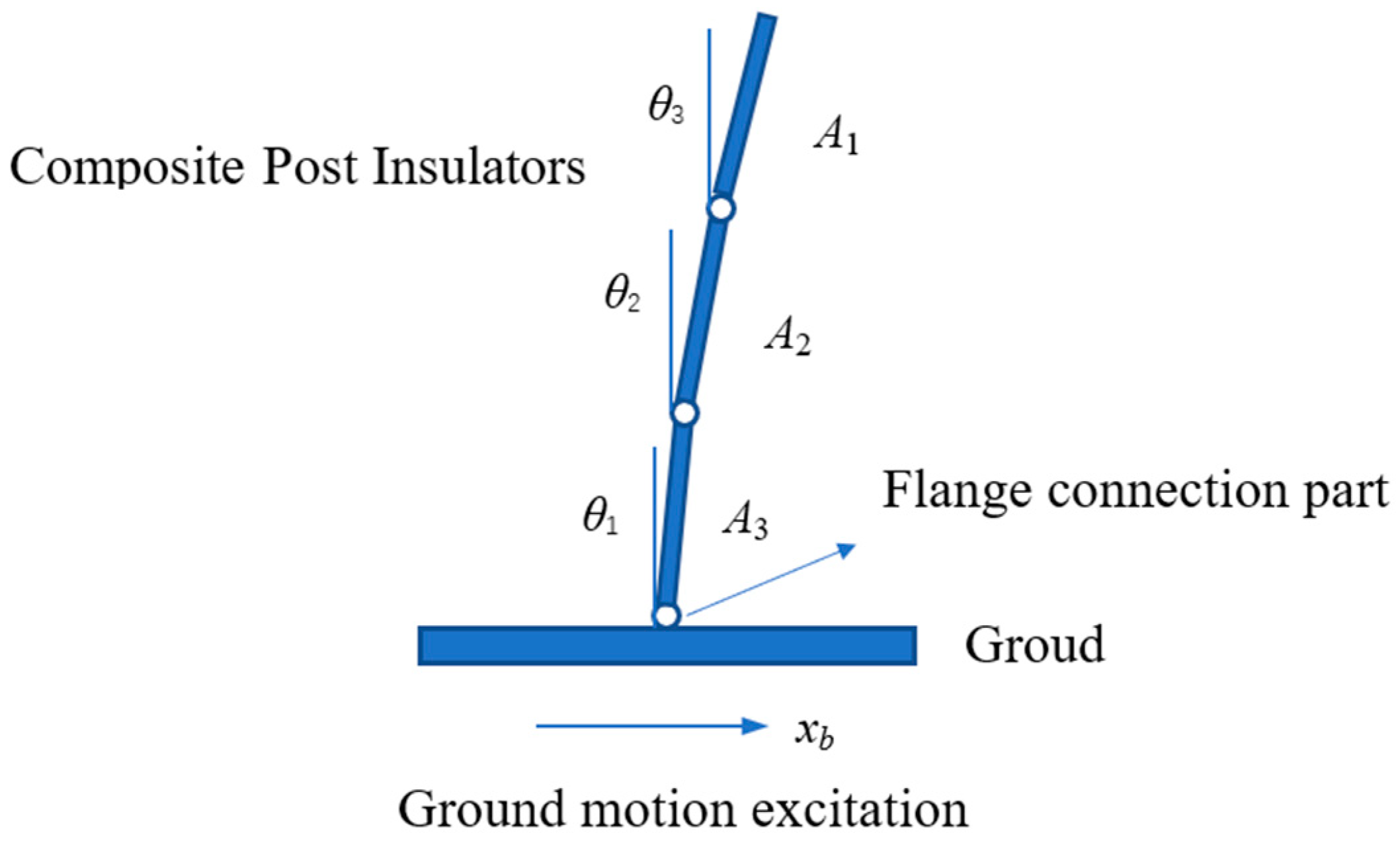
3. Dynamic Model of Composite Post Insulators under Earthquake

Composite post insulators are widely used in substations and are also an important component of substations. Figure 3 shows the composite post insulators used in substations.

To streamline the calculation process, this paper focuses on flanged three-section composite post insulators. Figure 4 shows an assembly diagram. Figure 5 illustrates the physical model of composite post insulators, with seismic excitation denoted as $x_b$. The physical parameters of the composite post insulators are given in

Table 1. Composite post insulator parameters.

Section	Length (mm)	Mass (kg)	Section Diameter (mm)	Flange Height h (mm)	Outer Diameter of Flange d (mm)
A1	3225	710	300	150	340
A2	2425	585	300	150	340
A3	2465	590	300	180	340

.

For a configuration of three post insulators, composite insulators are affixed with three flanges. Sections are joined by flanges, with one flange positioned at the upper end and another at the lower end of each connection (see Figure 4). The combined stiffness of the upper and lower flanges equals that of two springs arranged in series. Let the stiffness of the bottom flange of the upper composite insulator be represented by $k_{id}$, and the stiffness at the top of the lower insulator be denoted as $k_{(i-1)u}$. The resultant stiffness of the composite insulator’s two parts, denoted as $k_i$, can be expressed as follows [19,20]:

$$k_i=\frac{k_{id}{k}_{(i-1)u}}{k_{id}+k_{(i-1)u}}$$

(7)

According to the GB50260-2013 in China, the relationship between the bending stiffness of the upper and lower flanges of composite post insulator and flange mounting parameters, as well as modulus of the insulator, can be expressed as

$$K_c={\lambda }_c\frac{h_c}{d_c{E}_c}$$

(8)

where λ_c = 9.01 × 10⁷ E_c −5.09 × 10¹⁷ is the bending stiffness coefficient. h_c is the cemented height of the upper and lower flanges, d_c is the outer diameter at cemented parts of the composite insulator, and E_c is the modulus of the composite insulation. The parameters are presented in

Table 2. Bending stiffness parameters of composite post insulator flange.

Section	hc (m)	dc (m)	Ec (GPa)	Kc (N.m/rad)	λc
A1	0.15	0.34	68.7	3.7373 × 107	5.8213 × 1018
A2	0.15	0.34	65.5	3.8179 × 107	5.6645 × 1018
A3	0.18	0.34	67.8	4.9244 × 107	6.3052 × 1018

.

From the preceding analysis, the rotational bending moment stemming from the relative rotation of the upper and lower flanges can be represented as follows:

$$M_i=k_i({\theta }_i-{\theta }_{i-1})$$

(9)

Equation (9) delineates the rotational bending moment under ideal circumstances. The precise mechanics of rotational stiffness $k_i$ are intricate, encompassing the nonlinear mechanical traits of the cemented material and interfacial mechanics. In most prior investigations, the flange joint has been treated as a beam endowed with an equivalent rotational stiffness [21], factoring in large deformations within elastic theory. Following a sequence of mathematical simplifications, the nonlinear bending moment expression is derived.

$$M_i=k_i\left[({\theta }_i-{\theta }_{i-1})-\eta {({\theta }_i-{\theta }_{i-1})}^3\right]$$

(10)

Then, with the nonlinearity of the flange connection, the total elastic potential energy of flange connection can be expressed as

$$\begin{array}{c}{U}_k=\frac{1}{2}{k}_1{\theta }_1^2+\frac{1}{4}{\eta }_1{k}_1{\theta }_1^4+\frac{1}{2}{k}_2{\left({\theta }_2-{\theta }_1\right)}^2+\frac{1}{4}{\eta }_2{k}_2{\left({\theta }_2-{\theta }_1\right)}^4\\ +\frac{1}{2}{k}_3{\left({\theta }_3-{\theta }_2\right)}^2+\frac{1}{4}{\eta }_3{k}_3{\left({\theta }_3-{\theta }_2\right)}^4\end{array}$$

(11)

where

$$\begin{array}{l}{k}_1=k_{1d},\\ k_i=\frac{k_{id}{k}_{(i-1)u}}{k_{id}+k_{(i-1)u}},i=2,3\end{array}$$

(12)

The gravity potential energy of the composite post insulators changes due to the rotation of the composite post insulator, and the total gravity potential energy is

$$U_g=-\frac{1}{2}\left[\frac{1}{2}{m}_{1}g{L}_1{\theta }_1^2+m_{2}g(L_1{\theta }_1^2+\frac{1}{2}{L}_2{\theta }_2^2)+m_{3}g(L_1{\theta }_1^2+L_2{\theta }_2^2+\frac{1}{2}{L}_3{\theta }_3^2)\right]$$

(13)

The kinetic energy of composite post insulators includes translational kinetic energy and rotational kinetic energy, which are

$$T=\frac{1}{2}{m}_1{v}_{c1}^2+\frac{1}{2}{m}_2{v}_{c2}^2+\frac{1}{2}{m}_3{v}_{c3}^2+\frac{1}{2}\left(\frac{1}{12}{m}_1{L}_1^2{\dot{\theta }}_1^2+\frac{1}{12}{m}_2{L}_2^2{\dot{\theta }}_2^2+\frac{1}{12}{m}_3{L}_3^2{\dot{\theta }}_3^2\right)$$

(14)

where $v_{ci},i=1,2,3$ is the center of mass velocity of the i-th composite post insulator. The speed of the flange at the bottom of first composite post insulator is

$$v_0={\dot{x}}_b$$

(15)

The centroid speed of composite post insulator in section 1 is as follows:

$$v_{c1}=v_0+\frac{1}{2}{L}_1{\dot{\theta }}_1$$

(16)

The centroid speed of composite post insulator in section 2 is as follows:

$$v_{c2}=v_0+L_1{\dot{\theta }}_1+\frac{1}{2}{L}_2{\dot{\theta }}_2$$

(17)

The centroid speed of composite post insulator in section 3 is as follows:

$$v_{c3}=v_0+L_1{\dot{\theta }}_1+L_2{\dot{\theta }}_2+\frac{1}{2}{L}_3{\dot{\theta }}_3$$

(18)

According to the Hamilton principle, the Lagrange equation can be established:

$$\begin{array}{c}\left(\frac{1}{3}{m}_1+m_2+m_3\right)L_1^2{\ddot{\theta }}_1+\left(\frac{1}{2}{m}_2+m_3\right)L_1{L}_2{\ddot{\theta }}_2+\frac{1}{2}{m}_3{L}_1{L}_3{\ddot{\theta }}_3+k_1{\theta }_1-k_2\left({\theta }_2-{\theta }_1\right)\\ +k_1{\eta }_1{\theta }_1^3-k_2{\eta }_2{\left({\theta }_2-{\theta }_1\right)}^3-\left(\frac{1}{2}{m}_1+m_2+m_3\right)g{L}_1{\theta }_1=-\left(\frac{1}{2}{m}_1+m_2+m_3\right)L_1{\ddot{x}}_b\end{array}$$

$$\begin{array}{c}\left(\frac{1}{2}{m}_2+m_3\right)L_1{L}_2{\ddot{\theta }}_1+\left(\frac{1}{3}{m}_2+m_3\right)L_2^2{\ddot{\theta }}_2+\frac{1}{2}{m}_3{L}_2{L}_3{\ddot{\theta }}_3+k_2\left({\theta }_2-{\theta }_1\right)-k_3\left({\theta }_3-{\theta }_2\right)\\ +k_2{\eta }_2{\left({\theta }_2-{\theta }_1\right)}^3-k_3{\eta }_3{\left({\theta }_3-{\theta }_2\right)}^3-\left(\frac{1}{2}{m}_2+m_3\right)g{L}_2{\theta }_2=-\left(\frac{1}{2}{m}_2+m_3\right)L_2{\ddot{x}}_b\end{array}$$

(19)

$$\begin{array}{r}\frac{1}{2}{m}_3{L}_1{L}_3{\ddot{\theta }}_1+\frac{1}{2}{m}_3{L}_2{L}_3{\ddot{\theta }}_2+\frac{1}{3}{m}_3{L}_3^2{\ddot{\theta }}_3+k_3\left({\theta }_3-{\theta }_2\right)+k_3{\eta }_3{\left({\theta }_3-{\theta }_2\right)}^3\\ -\frac{1}{2}{m}_{3}g{L}_3{\theta }_3=-\frac{1}{2}{m}_3{L}_3{\ddot{x}}_b\end{array}$$

Considering the damping in the structure, Equation (19) can be written in matrix form as follows:

$$\mathit{M}\ddot{\mathbf{\theta }}+\mathit{C}\dot{\mathbf{\theta }}+\mathit{K}\mathbf{\theta }+\mathit{G}(\mathbf{\theta })=\mathit{F}{\ddot{x}}_b$$

(20)

where C = 2ζ MΦΛΦ⁻¹, ζ is the damping ratio, Φ is the modal matrix, and Λ is the diagonal matrix formed by the natural frequency:

$$\begin{array}{l}\mathit{M}=\left[\begin{array}{ccc}\left(\frac{1}{3}{m}_1+m_2+m_3\right)L_1^2& \left(\frac{1}{2}{m}_2+m_3\right)L_1{L}_2& \frac{1}{2}{m}_3{L}_1{L}_3\\ \left(\frac{1}{2}{m}_2+m_3\right)L_1{L}_2& \left(\frac{1}{3}{m}_2+m_3\right)L_2^2& \frac{1}{2}{m}_3{L}_2{L}_3\\ \frac{1}{2}{m}_3{L}_1{L}_3& \frac{1}{2}{m}_3{L}_2{L}_3& \frac{1}{3}{m}_3{L}_3^2\end{array}\right]\\ \mathit{K}=\left[\begin{array}{ccc}{k}_1+k_2-\left(\frac{1}{2}{m}_1+m_2+m_3\right)g{L}_1& -k_2& 0\\ -k_2& k_2+k_3-\left(\frac{1}{2}{m}_2+m_3\right)g{L}_2& -k_3\\ 0& -k_3& k_3-\frac{1}{2}{m}_{3}g{L}_3\end{array}\right]\\ \mathit{G}(\mathbf{\theta })=\left\{\begin{array}{c}{k}_1{\eta }_1{\theta }_1^3-k_2{\eta }_2{\left({\theta }_2-{\theta }_1\right)}^3\\ k_2{\eta }_2{\left({\theta }_2-{\theta }_1\right)}^3-k_3{\eta }_3{\left({\theta }_3-{\theta }_2\right)}^3\\ k_3{\eta }_3{\left({\theta }_3-{\theta }_2\right)}^3\end{array}\right\}\hspace{1em}\mathit{F}=f\left\{\begin{array}{c}-\left(\frac{1}{2}{m}_1+m_2+m_3\right)L_1\\ -\left(\frac{1}{2}{m}_2+m_3\right)L_2\\ -\frac{1}{2}{m}_3{L}_3\end{array}\right\}\end{array}$$

(21)

4. Analytical Study

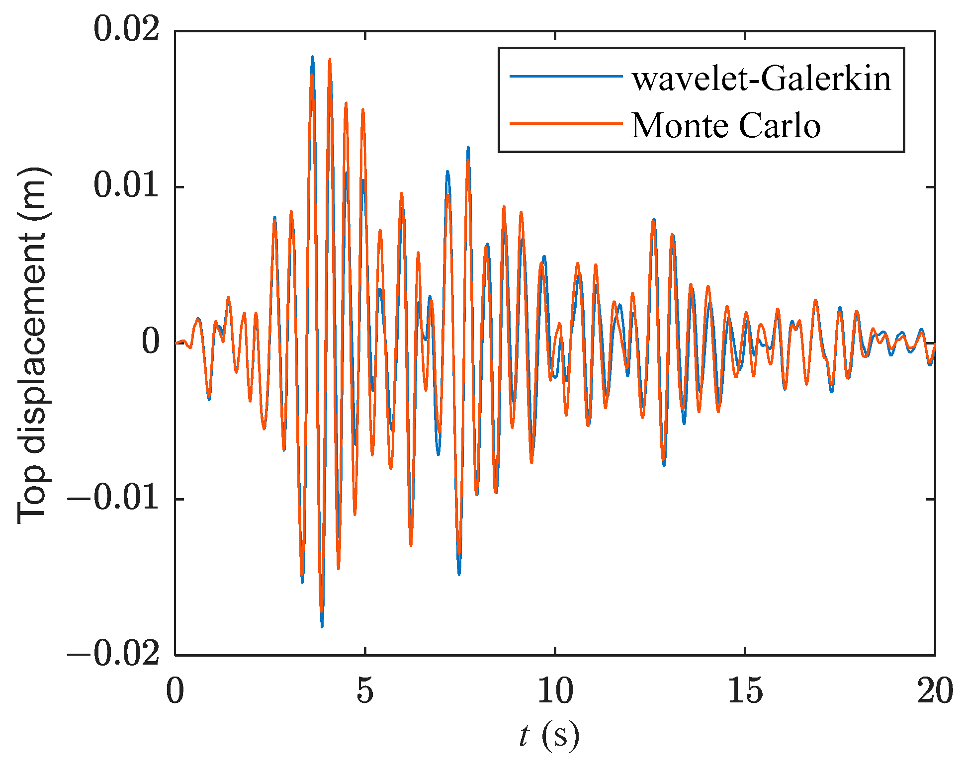
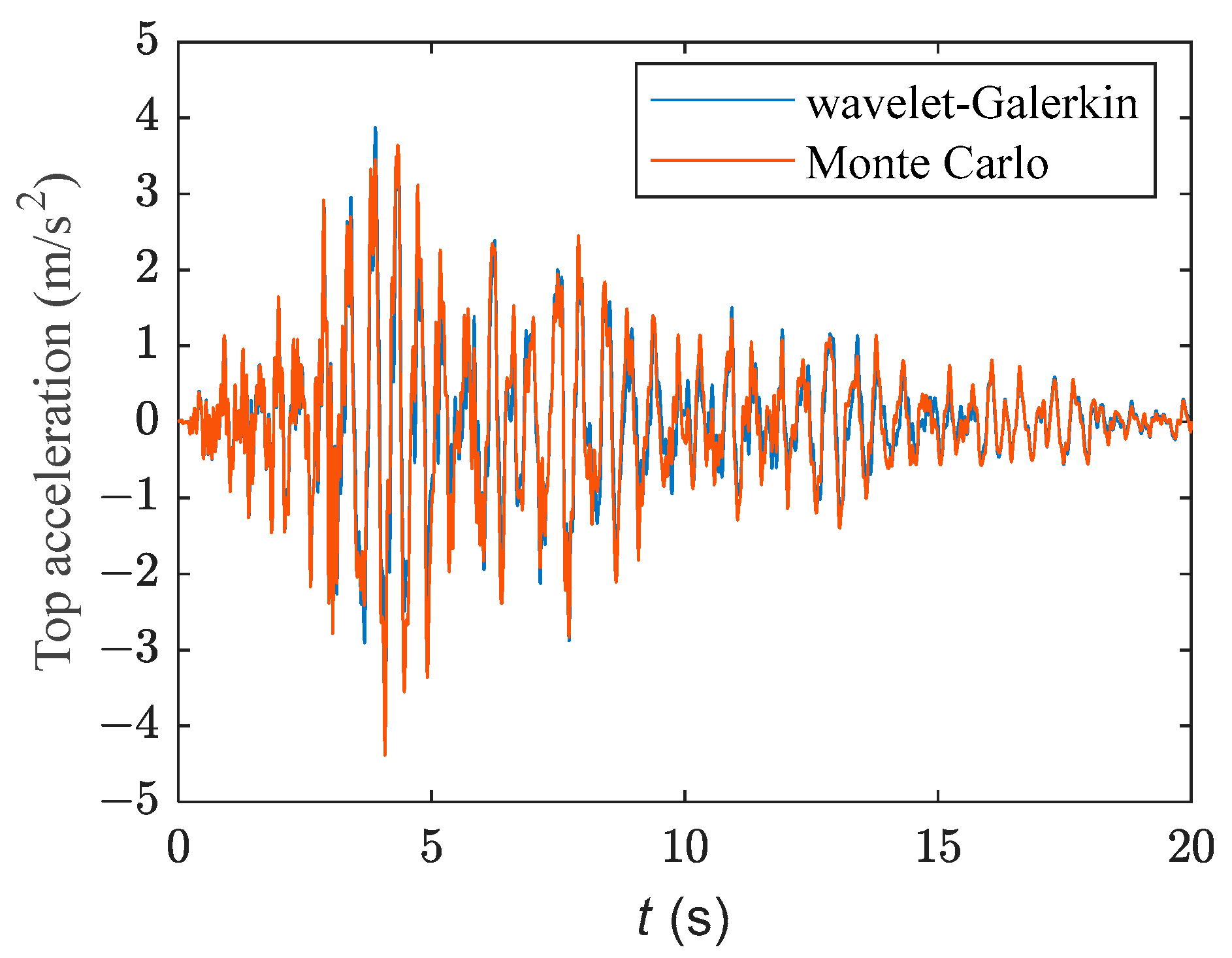
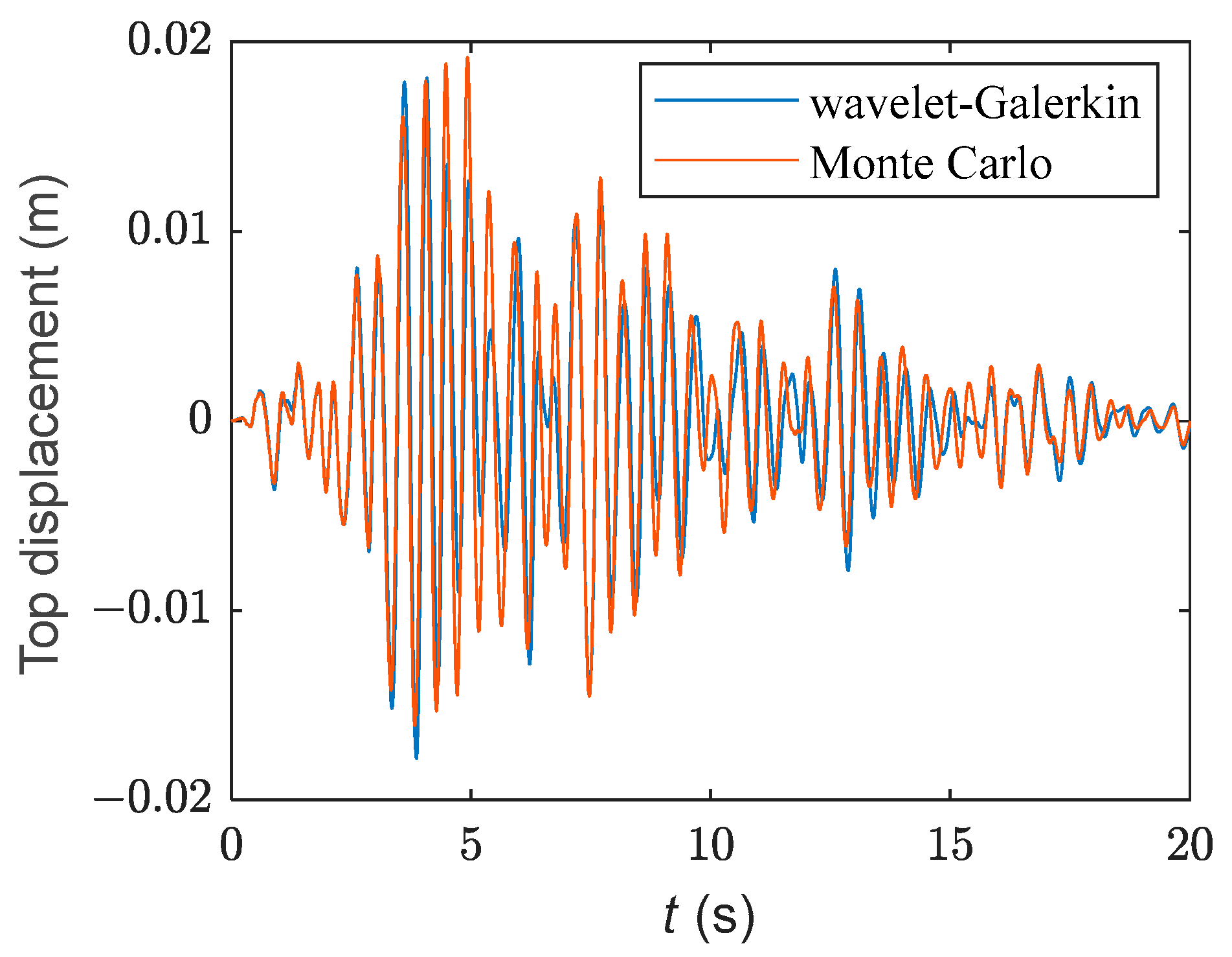
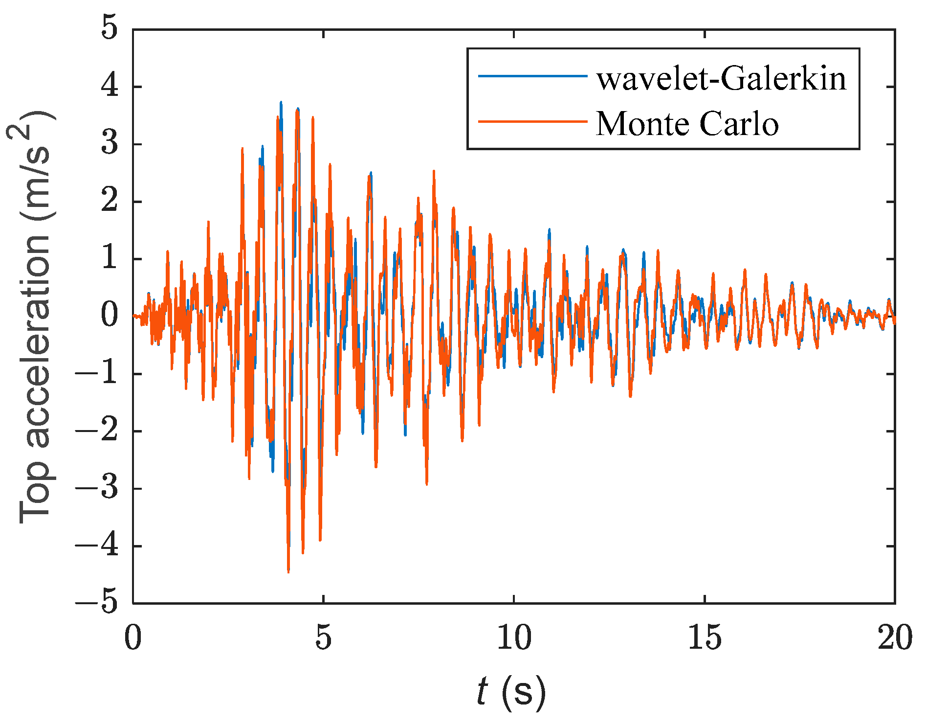
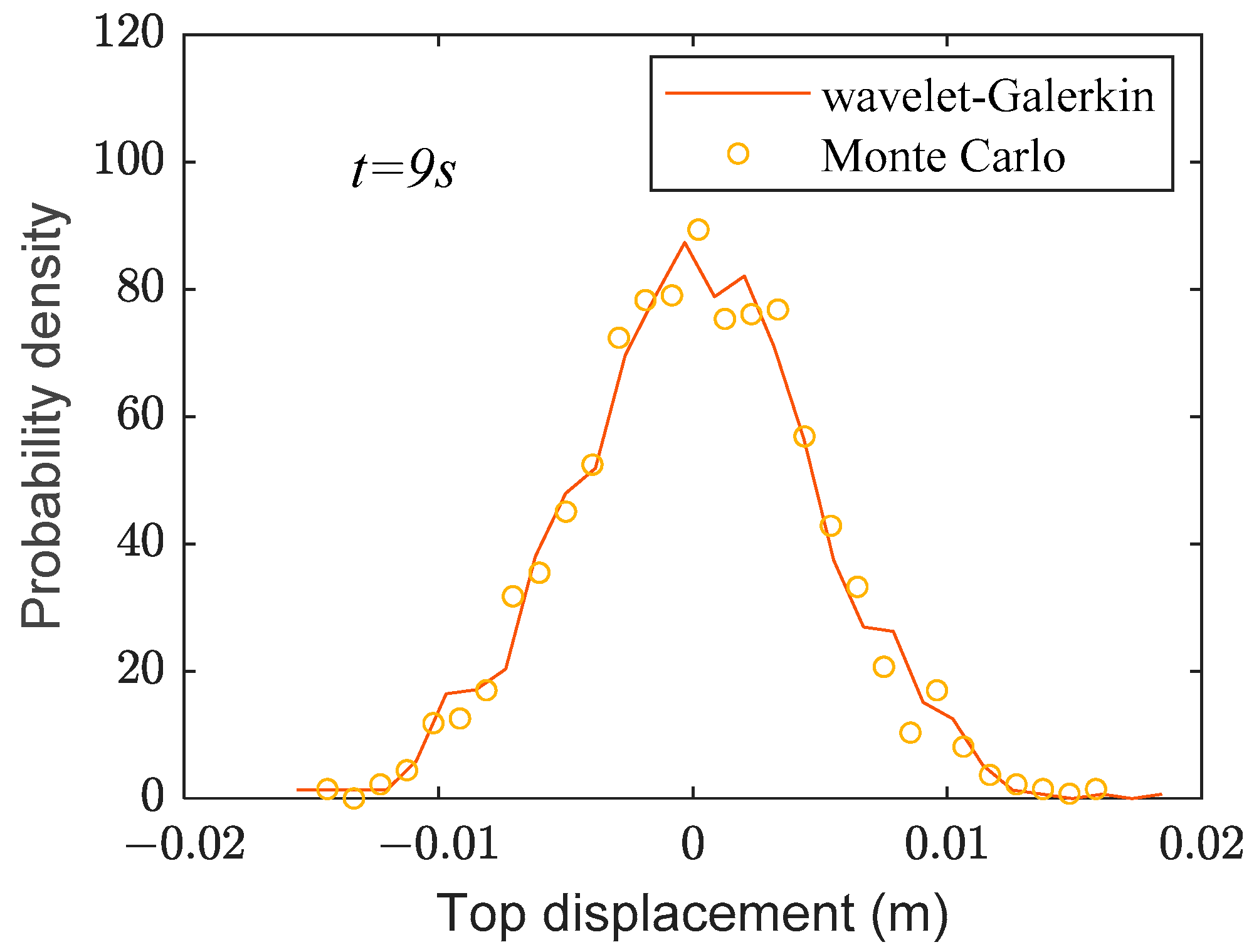
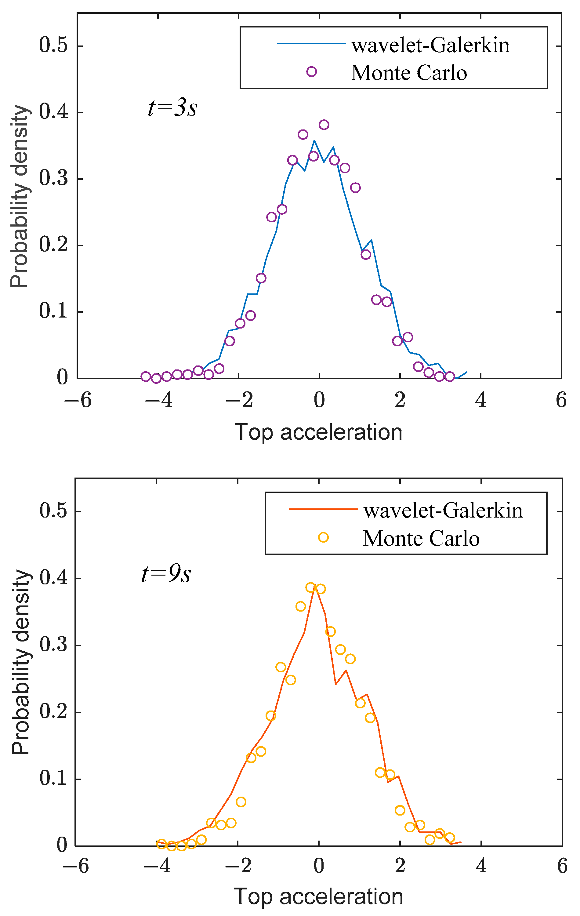
4.1. Seismic Response

Due to the non-stationary nature of ground motion excitation, the wavelet-Galerkin method [12] is employed to solve the response of the system (20), and the wavelet expansion of Equation (20) is performed:

$$\begin{array}{ll}\mathit{M}{\displaystyle \sum _i{\displaystyle \sum _k\left\{{\mathit{W}}_{i,k}^{\mathbf{\theta }}{\ddot{\psi }}_{i,k}(t)\right.}}\left.+{\tilde{\mathit{W}}}_{i,k}^{\mathbf{\theta }}{\ddot{\overline{\psi }}}_{i,k}(t)\right\}& +\mathit{C}{\displaystyle \sum _i{\displaystyle \sum _k\left\{{\mathit{W}}_{i,k}^{\mathbf{\theta }}{\dot{\psi }}_{i,k}(t)+{\tilde{\mathit{W}}}_{i,k}^{\mathbf{\theta }}{\dot{\overline{\psi }}}_{i,k}(t)\right\}}}\\ & +\mathit{K}{\displaystyle \sum _i{\displaystyle \sum _k\left\{{\mathit{W}}_{i,k}^{\mathbf{\theta }}{\psi }_{i,k}(t)+{\tilde{\mathit{W}}}_{i,k}^{\mathbf{\theta }}{\overline{\psi }}_{i,k}(t)\right\}}}+G(\mathbf{\theta })=\mathit{W}(t)\end{array}$$

(22)

where ${\mathit{W}}_{i,k}^{\mathbf{\theta }}$ is the wavelet coefficient vector of the dynamic response at the i-th scale and k-th time translation. In the case where the dynamic response is a real value process, ${\tilde{\mathit{W}}}_{i,k}^{\mathbf{\theta }}$ is the conjugate of ${\mathit{W}}_{i,k}^{\mathbf{\theta }}$. ${\psi }_{i,k}$ is the wavelet function at scale i-th and k-th time translation and ${\overline{\psi }}_{i,k}$ are the conjugates of wavelet functions. Multiply both sides of Equation (22) by ${\overline{\psi }}_{i,k}$ and integrate over the interval $[0,T_0]$ with respect to $t$ to obtain

$$\begin{array}{l}\mathit{M}{\displaystyle \sum _i{\displaystyle \sum _k{\displaystyle {\int }_0^{T_0}\left\{{\mathit{W}}_{i,k}^{\mathbf{\theta }}{\ddot{\psi }}_{i,k}(t)+{\tilde{W}}_{i,k}^{\mathbf{\theta }}{\ddot{\overline{\psi }}}_{i,k}(t)\right\}}}}{\overline{\psi }}_{j,l}(t)\mathrm{d}t\\ +C{\displaystyle \sum _i{\displaystyle \sum _k{\displaystyle {\int }_0^{T_0}\left\{{\mathit{W}}_{i,k}^{\mathbf{\theta }}{\dot{\psi }}_{i,k}(t)+{\tilde{W}}_{i,k}^{\mathbf{\theta }}{\dot{\overline{\psi }}}_{i,k}(t)\right\}}}}{\overline{\psi }}_{j,l}(t)\mathrm{d}t\\ +K{\displaystyle \sum _i{\displaystyle \sum _k{\displaystyle {\int }_0^{T_0}\left\{{\mathit{W}}_{i,k}^{\mathbf{\theta }}{\psi }_{i,k}(t)+{\tilde{W}}_{i,k}^{\mathbf{\theta }}{\overline{\psi }}_{i,k}(t)\right\}}}}{\overline{\psi }}_{j,l}(t)\mathrm{d}t\\ +{\displaystyle {\int }_0^{T_0}G(\mathbf{\theta })}{\overline{\psi }}_{j,l}(t)\mathrm{d}t={\displaystyle {\int }_0^{T_0}W}(t){\overline{\psi }}_{j,l}(t)\mathrm{d}t\end{array}$$

(23)

Due to orthogonality,

$$\begin{array}{l}{\displaystyle {\int }_0^{T_0}{\overline{\psi }}_{i,k}}(t){\overline{\psi }}_{j,l}(t)\mathrm{d}t=0\\ {\displaystyle {\int }_0^{T_0}{\dot{\overline{\psi }}}_{i,k}}(t){\overline{\psi }}_{j,l}(t)\mathrm{d}t=0\\ {\displaystyle {\int }_0^{T_0}{\ddot{\overline{\psi }}}_{i,k}}(t){\overline{\psi }}_{j,l}(t)\mathrm{d}t=0\end{array}$$

(24)

Equation (23) can be simplified as

$${\displaystyle \sum _i{\displaystyle \sum _k{\mathit{W}}_{i,k}^x}}{\mathit{A}}_{i,k;j,l}+{\displaystyle {\int }_0^{T_0}G(\mathbf{\theta })}{\overline{\psi }}_{j,l}(t)\mathrm{d}t=\frac{T_0}{n-m}{\mathit{W}}_{j,l}^w$$

(25)

where ${\mathit{A}}_{i,k;j,l}=C_{i,k;j,l}^2\mathit{M}+C_{i,k;j,l}^1\mathit{C}+C_{i,k;j,l}^0\mathit{K}$,

$$\begin{array}{l}{C}_{i,k;j,l}^0={\displaystyle {\int }_0^{T_0}{\psi }_{i,k}(t){\overline{\psi }}_{j,k}(t)dt}=\left\{\begin{array}{cc}\frac{T_0}{{(n-m)}^2}{\displaystyle \sum _{q=m_i}^{n_i-1}{e}^{\mathrm{i}2\pi q\frac{1-k}{n-m}}},& i=j\\ 0,& \mathrm{else} \end{array}\right.\\ C_{i,k;j,l}^1={\displaystyle {\int }_0^{T_0}{\dot{\psi }}_{i,k}(t)}{\overline{\psi }}_{j,k}(t)dt=\left\{\begin{array}{cc}\frac{i2\pi }{{(n-m)}^2}{\displaystyle \sum _{q=m_i}^{n_i-1}q}{e}^{\mathrm{i}2\pi q(l-k/n-m)},& i=j\\ 0,& \mathrm{else} \end{array}\right.\\ C_{i,k;j,l}^2={\displaystyle {\int }_0^{T_0}{\ddot{\psi }}_{i,k}(t)}{\overline{\psi }}_{j,k}(t)dt=\left\{\begin{array}{cc}\frac{-2\pi \Delta \omega }{{(n-m)}^2}{\displaystyle \sum _{q=m_i}^{n_i-1}{q}^2}{e}^{\mathrm{i}2\pi q(l-k/n-m)},& i=j\\ 0,& \mathrm{else} \end{array}\right.\end{array}$$

(26)

Equation (25) can be simplified into a matrix form:

$${\mathit{A}}^j{\mathit{W}}^{j,x}+{\mathit{G}}^j=\frac{T_0}{n-m}{\mathit{W}}^{j,\mathit{W}}$$

(27)

In the linear scenario, the system response can be directly obtained from Equation (27). The predictions regarding the top displacement and top acceleration of composite post insulators are depicted in Figure 6 and Figure 7, with the parameters ${\eta }_i=0(i=1,2,3)$, while the others are given in Table 1 and Table 2.

In the event of considering the nonlinear case, the Newton iteration method [12] is employed to acquire the system response. The transformation of Equation (27) is as follows:

$$\begin{array}{ll}{\mathrm{F}}_l^j(\alpha )& =\mathrm{F}((j-1)(n-m)+(l+1))\\ & ={\displaystyle \sum _k{W}_k^{j,\mathbf{\theta }}}{A}_{k;l}^j+{\displaystyle {\int }_0^{T_0}G}(\mathbf{\theta }){\overline{\psi }}_{j,l}(t)\mathrm{d}t-\frac{T_0}{n-m}{W}_l^{j,w}=0\\ & \left(j=1,2,\cdots ,N_{\mathsf{\Omega }};k,l=0,1,\cdots ,N_t-1;\right)\end{array}$$

(28)

where ${\mathrm{F}}_l^j(\alpha )$ represents the vector element at the l-th time translation on the j-th scale. The Newton iteration method requires solving the following iterative equations:

$$\mathit{F}\left({\alpha }^{(n)}\right)+\Delta \mathit{F}\left({\alpha }^{(n)}\right)\left({\alpha }^{(n+1)}-{\alpha }^{(n)}\right)=0$$

(29)

where

$$\alpha ={\left[W_{1,0}^{\mathit{x}},W_{1,1}^{\mathit{x}},\cdots ,W_{1,n_d{N}_{\epsilon }-1}^{\mathit{x}},W_{2,0}^{\mathit{x}},W_{2,1}^{\mathit{x}},\cdots ,W_{2,n_d{N}_t-1}^{\mathit{x}},\dots ,W_{N_{\mathsf{\Omega }},0}^{\mathit{x}},W_{N_{\mathsf{\Omega }},1}^{\mathit{x}},\cdots ,W_{N_{\mathsf{\Omega }},n_d{N}_t-1}\right]}^{\mathrm{x}},$$

(30)

$\Delta \mathit{F}(\alpha )$ is Jacobian matrix, which can be decomposed into linear and nonlinear parts, namely

$$[\Delta \mathit{F}(\alpha )]=\frac{\partial \mathit{F}(\alpha )}{\partial \alpha }={[\Delta \mathit{F}(\alpha )]}_L+{[\Delta \mathit{F}(\alpha )]}_{NI}$$

(31)

$${[\Delta \mathit{F}(\alpha )]}_L=\left[\begin{array}{cccc}{\mathit{A}}^1& 0& \cdots & 0\\ 0& {\mathit{A}}^2& \cdots & 0\\ ⋮& ⋮& \ddots & ⋮\\ 0& 0& 0& {\mathit{A}}^{N_{\mathsf{\Omega }}}\end{array}\right]$$

(32)

$$\begin{array}{c}{[\Delta \mathit{F}(\alpha )]}_{NL}((j-1)(n-m)+(l+1),(i-1)(n-m)+(k+1))={\displaystyle {\int }_0^{T_0}\frac{\partial \mathit{G}(\mathbf{\theta })}{\partial W_{i,k}^{\mathbf{\theta }}}}{\overline{\psi }}_{j,l}(t)\mathrm{d}t\\ ={\displaystyle {\int }_0^{T_0}\frac{\partial \mathit{G}}{\partial \mathbf{\theta }}\frac{\partial \mathbf{\theta }}{\partial W_{i,k}^{\mathbf{\theta }}}}{\overline{\psi }}_{j,l}(t)\mathrm{d}t={\displaystyle {\int }_0^{T_0}\frac{\partial \mathit{G}}{\partial \mathbf{\theta }}{\psi }_{i,k}(t)}{\overline{\psi }}_{j,l}(t)\mathrm{d}t\end{array}$$

(33)

The system response can be obtained by solving the iterative Equation (33). Figure 8 and Figure 9 show the top displacement and acceleration of composite post insulators, respectively, where the parameters are $T_0=20$, $N=1024$, $\Delta t=[0,T_0)$, $\Delta t=0.02$, ${\omega }_{\max }=\pi /\Delta t$, $\Delta \omega =2{\omega }_{\max }/N$, and $N_t=n-m=32$. The other parameters are the same as in the linear case.

Figure 10 and Figure 11 show the instantaneous probability density distribution of the top displacement and top acceleration of composite post insulator at different times, 3 s and 9 s, respectively. The comparison between the results from the wavelet-Galerkin method and those from the numerical simulation in Figure 6, Figure 7, Figure 8, Figure 9, Figure 10 and Figure 11 demonstrates a strong agreement, indicating the efficacy of this strategy in predicting the dynamic response of pillar-type electrical equipment under stochastic ground motion, encompassing both amplitude and frequency non-stationarities.

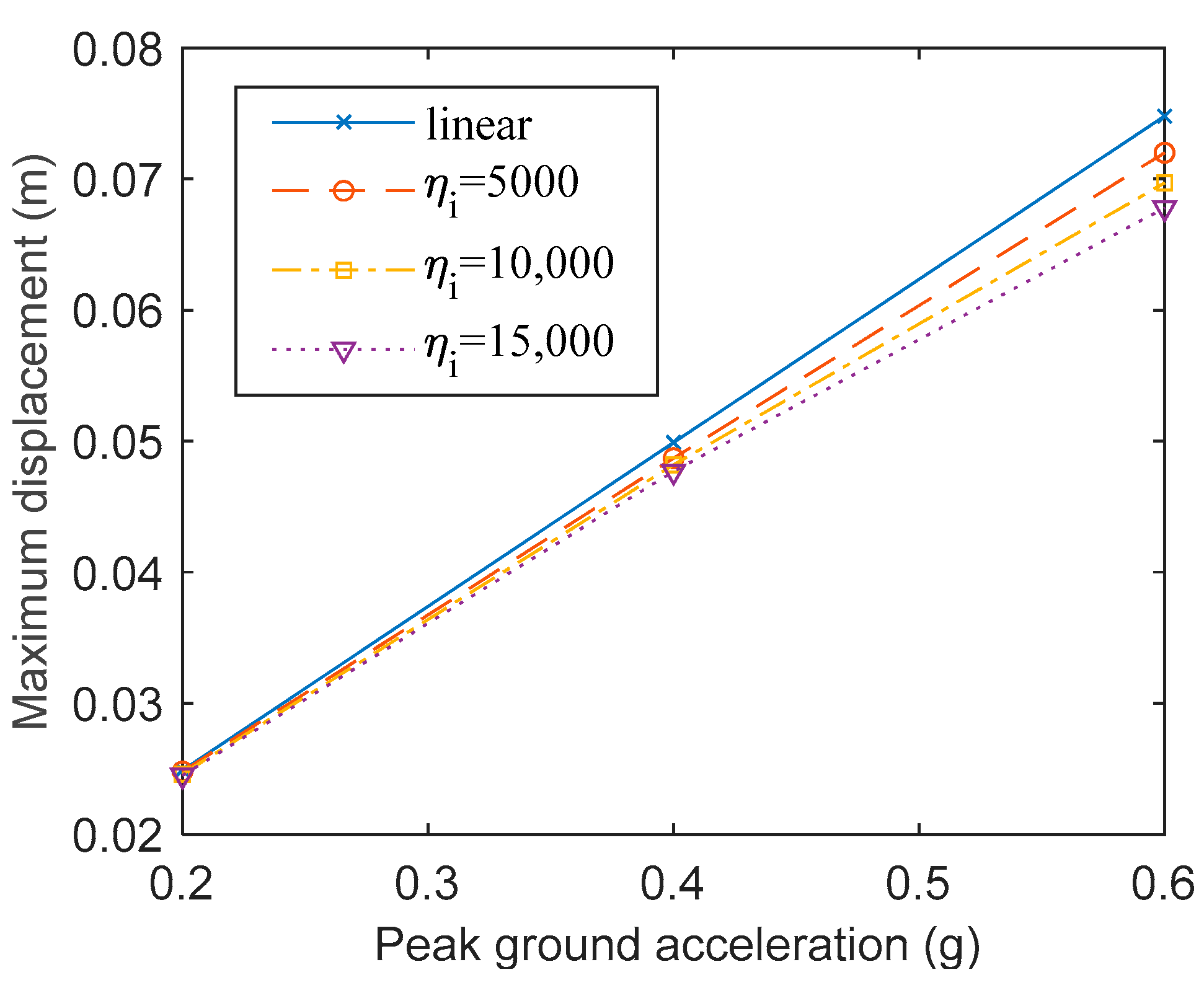
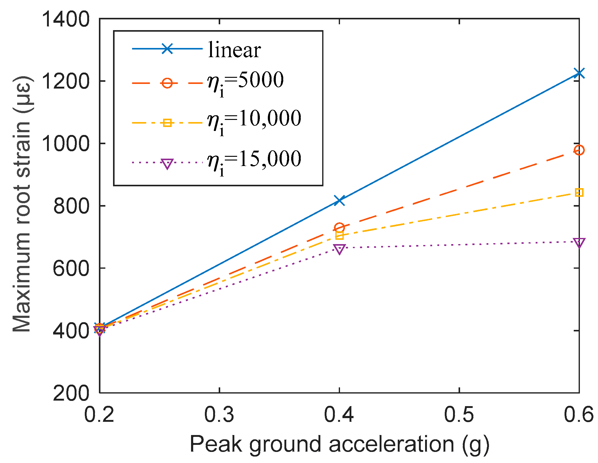
4.2. The Impact of Nonlinearity on System Response

Composite post insulators, as a novel and evolving technology, have a very complex mechanical behavior due to their materials and connections. The main manifestation is the nonlinear phenomenon of stiffness. Consequently, the influence of nonlinear stiffness on system response will be investigated.

Initially, we investigate the influence of different nonlinear stiffness coefficients ${\eta }_i=5000, 10000, 15000(i=1,2,3)$ on the system response, focusing on two critical parameters: the maximum top displacement and the maximum root strain of the composite post insulators. The former directly reflects the vibration amplitude of the system under seismic action, while the latter holds paramount importance in seismic design, given that fractures in composite post insulators typically occur at the root. The level of root strain significantly influences the likelihood of fracture in the composite post insulators [22].

Figure 12 and Figure 13 depict the maximum top displacement and maximum root strain of composite post insulators under various peak ground accelerations (0.2 g, 0.4 g, 0.6 g) using the method proposed in Section 4.1. A notable disparity in system response between linear and nonlinear stiffness is evident. Under linear stiffness conditions, both the maximum displacement and maximum root strain exhibit linear growth with increasing peak ground acceleration. However, upon considering nonlinear factors, the growth in maximum displacement and maximum root strain becomes nonlinear, with the magnitude of increase gradually diminishing.

Figure 12 and Figure 13 illustrate that the nonlinear seismic response of the equipment is comparatively smaller than its linear counterpart when subjected to seismic excitation. Moreover, as the ground motion excitation intensifies, the contrast between the nonlinear and linear response of the equipment becomes more pronounced. This observation suggests that the equipment demonstrates increasingly evident nonlinear characteristics with higher levels of seismic excitation. For example, when the peak ground acceleration increases from 0.2 g to 0.6 g, the maximum top displacement increases from 24.9 mm to 74.8 mm without considering nonlinear factors; however, with the inclusion of nonlinear factors ${\eta }_i=15000$, this range reduces to from 24.5 mm to 67.8 mm. Correspondingly, the variation range of the maximum root strain is from 408.5 $\mathsf{\mu }\mathsf{\epsilon }$ to 1225.5 $\mathsf{\mu }\mathsf{\epsilon }$ and from 401.9 $\mathsf{\mu }\mathsf{\epsilon }$ to 685 $\mathsf{\mu }\mathsf{\epsilon }$, respectively.

Table 3. The difference in top displacement and root strain between linear and different nonlinear parameters.

		Difference Range ((Linear − Nonlinear)%/Linear)
		Seismic Excitation	ηi = 5000	ηi = 10,000	ηi = 15,000
Top displacement		0.2 g	0.4	0.8	1.6
		0.4 g	2.4	3.4	4.4
		0.6 g	3.7	6.8	9.4
Root strain		0.2 g	0.5	10.7	20.1
		0.4 g	1	13.8	31.3
		0.6 g	1.6	18.6	44.1

provides the percentages of the difference between the nonlinear analysis results and linear analysis results of displacement when the peak ground acceleration is 0.2 g, 0.4 g, and 0.6 g. As the seismic excitation intensifies, the impact of nonlinearity progressively amplifies. For instance, with a nonlinear stiffness of ${\eta }_i=5000$, the difference range between 0.2 g and 0.6 g only increases by 3.3%, whereas with a nonlinear stiffness of ${\eta }_i=15000$, this difference surges by 7.8% between 0.2 g and 0.6 g.

As depicted in Figure 13, the influence of nonlinearity on root stress becomes increasingly pronounced with the escalation of seismic excitation. Initially, when the peak ground acceleration is 0.2 g, nonlinearity exerts minimal impact on root stress. However, as the excitation intensity amplifies, the disparity in root stress between nonlinear and linear scenarios gradually magnifies. By the time the peak ground acceleration reaches 0.6 g, the disparity reaches values of 1.6%, 18.6%, and 44.1% with varying nonlinear stiffness coefficients, ${\eta }_i=5000, 10000, 15000$, respectively.

The percentages of the difference between the nonlinear analysis results and linear analysis results of the maximum root strain are given in Table 3. It is evident that nonlinearity exerts a substantial influence on root stress, particularly under high excitation intensities, and this effect amplifies with increasing nonlinearity. Notably, the difference between nonlinear and linear scenarios peaks reached an astonishing level at 44.1% when the peak ground acceleration reached 0.6 g with stiffness coefficients ${\eta }_i=15000$.

Additionally, Figure 13 reveals that higher levels of nonlinear stiffness result in seismic excitations having minimal impact on the maximum root strain of the composite post insulators, eventually stabilizing. This indicates that the influence of nonlinear stiffness on the maximum root strain of composite post insulators under high seismic excitation is larger and the maximum root strain changes rapidly. When the nonlinear stiffness increases to a certain value, the impact of nonlinear stiffness on the maximum root strain is rather small, and the root strain change in the composite post insulators has entered a stationary change. This observed trend is similar to the seismic vibration response results of 1100 kV composite pillar insulators [6], reflecting the experimental characteristics of their nonlinear bending stiffness [23].

Drawing from the preceding analysis, it is evident that nonlinear factors exert a substantial influence on the response of composite post insulators, necessitating their consideration in seismic design. The pivotal criterion for assessing the seismic safety of post insulator electrical equipment revolves around whether the root strain exceeds the safety limits. As evidenced by Figure 13 and Table 3, nonlinearity notably affects the root strain of composite post insulators.

The nonlinear stiffness of a structure is influenced by various factors, including material nonlinearity, geometric nonlinearity, and the nonlinearity at adhesive joints between composite materials and flanges. These factors collectively affect the structural response. Traditionally, experimental methods have been used to determine their impact, but physical experiments are costly and time-consuming. To address this, the impact of nonlinearity could be analyzed firstly through theoretical methods by, for instance, utilizing the theoretical method proposed in this paper. Subsequently, one could conduct complementary theoretical analyses with corresponding experiments. This combined approach is invaluable for establishing requirements in future seismic design.

5. Conclusions

This paper accomplishes two main tasks: firstly, it establishes a stochastic-excited nonlinear dynamic model for composite post insulators under earthquake conditions. The seismic motion model incorporates randomness and non-stationarity of amplitude and frequency, tailored for Chinese power facilities. When predicting the stochastic response of a nonlinear dynamic system under seismic excitation, one encounters two primary challenges: the stochastic and non-stationarity of excitation and strong nonlinearity of the system. Therefore, the second task involves successfully applying the stochastic dynamic method to this model, yielding dynamic responses.

These achievements enable an analysis of the impact of structural nonlinearity on system response. The findings reveal that the nonlinear calculation results of both the maximum top displacement and the maximum root strain of composite post insulators are smaller than the linear calculation results. As seismic excitation increases, the disparity between these results grows, particularly regarding maximum root strain, where the difference becomes more pronounced. Once the nonlinear stiffness reaches a certain threshold, its influence on the maximum root strain of composite post insulators diminishes, and the strain change stabilizes.

In light of these conclusions, the random seismic motion model and nonlinear stochastic dynamics method proposed in this paper offer valuable insights for the seismic design of power facilities.

References

1. Ying, Z.G.; Ni, Y.Q.; Ko, J.M. Semi-active optimal control of linearized systems with multi-degree of freedom and application. J. Sound. Vib. 2005, 279, 373–388. [Google Scholar] [CrossRef]
2. Qian, J.; Yang, J.P.; Xia, Y.; Yan, Y.X.; Zhou, J.T. Rapid damage assessment of regional beam bridges after earthquake based on simplified models and different seismic inputs. Structures 2023, 57, 105306. [Google Scholar] [CrossRef]
3. Kempner, L.; Scott, M.S.; Haldar, A.K. Seismic Effects on Transmission Lines and Their Major Components. Electr. Transm. Substn. Struct. 2018, 2018, 132–145. [Google Scholar]
4. He, C.; Xie, Q.; Yang, Z.Y.; Xue, S.T. Seismic evaluation and analysis of 1100-kVUHV porcelain transformer bushings. Soil Dyn. Earthq. Eng. 2019, 123, 498–512. [Google Scholar] [CrossRef]
5. Liu, H.; Chen, Y.; Lu, Z.; Zhu, Z. Shaking Table Test of a ±1100 k V Composite Post Insulator. Insul. Surg. Arrest. 2018, 138–144. [Google Scholar]
6. Kanai, K. Semi-Empirical Formula for the Seismic Characteristics of the Ground. Bull. Earthq. Res. Inst. Univ. Tokyo 1957, 35, 309–325. [Google Scholar]
7. Clough, R.W.; Penzien, J. Dynamics of Structures. McGraw-Hill Book, Co.: New York, NY, USA, 1975. [Google Scholar]
8. Ou, J.P.; Niu, D.T. Parameters in the Random Process Models of Earthquake Ground Motion and their Effects on the Response of Structures. J. Harbin Eng. Univ. 1990, 23, 24–34. [Google Scholar]
9. Liu, Z.J.; Liu, Z.H.; Liu, W. Probability Model of Fully Non-stationary Ground Motion with the Target Response Spectrum Compatible. J. Vib. Shock 2017, 36, 32–38. [Google Scholar]
10. Gumus, E.; Ozturk, B.; Mohamed Nazri, F. Scaling method application for seismic design along the central Anatolian fault zone. Adv. Civ. Eng. 2022, 2022, 1963553. [Google Scholar] [CrossRef]
11. GB50260-2013; Code for Seismic Design of Electrical Installations. Ministry of Housing and Urban-Rural Development: Beijing, China, 2013.
12. Han, X.; Pagnacco, E. Response EPSD of chain-like MDOF nonlinear structural systems via wavelet-Galerkin method. Appl. Math. Model. 2022, 103, 475–492. [Google Scholar] [CrossRef]
13. Hashemi AMosalam, K.M. Shake-table experiment on reinforced concrete structure containing masonry infill wall. Earthq. Eng. Struct. D 2006, 35, 1827–1852. [Google Scholar] [CrossRef]
14. John, D.; Aochi, H. A survey of techniques for predicting earthquake ground motions for engineering purposes. Surv. Geophys. 2008, 29, 187–220. [Google Scholar]
15. Wilson, E.; Der Kiureghian, A.; Bayo, E.P. A Replacement for The Srss Method Inseismic Analysis. Earthq. Eng. Struct. D 1981, 9, 187. [Google Scholar] [CrossRef]
16. Shinozuka, M.; Sato, Y. Simulation of nonstationary random processes. ASCE J. Eng. Mech. Div. 1967, 93, 11–40. [Google Scholar] [CrossRef]
17. Jun, X.; Wang, J.; Wang, D. Evaluation of the probability distribution of the extreme value of the response of nonlinear structures subjected to fully nonstationary stochastic seismic excitations. J. Eng. Mech. 2020, 146, 06019006. [Google Scholar]
18. Fabio, S.; Antonio, P.; Gabriele, F.; Giovanni, L.; Lucia, L. Simulation of non-stationary stochastic ground motions based on recent Italian earthquakes. Bull. Earthq. Eng. 2021, 19, 3287–3315. [Google Scholar]
19. Xue, Y.; Cheng, Y.; Zhu, Z.; Li, S.; Liu, Z.; Guo, H.; Zhang, S. Study on Seismic Performance of Porcelain Pillar Electrical Equipment Based on Nonlinear Dynamic Theory. Adv. Civ. Eng. 2021, 2021, 8816322. [Google Scholar] [CrossRef]
20. Zhu, Z.; Zhang, L.; Cheng, Y.; Guo, H.; Lu, Z. On the Nonlinear Seismic Responses of Shock Absorber-Equipped Porcelain Electrical Components. Math. Probl. Eng. 2020, 2020, 9026804. [Google Scholar] [CrossRef]
21. Paolacci, F.; Giannini, R. Seismic reliability assessment of a high-voltage disconnect switch using an effective fragility analysis. J. Earthq. Eng. 2009, 13, 217–235. [Google Scholar] [CrossRef]
22. Roh, H.; Nicholas, D.O.; Andrei, M.R. Experimental test and modeling of hollow-core composite insulators. Nonlinear Dynam. 2012, 69, 1651–1663. [Google Scholar] [CrossRef]
23. Liu, H.; Cheng, Y.; Lu, Z.; Zhu, Z.; Li, S. Study on the Flexural Behavior of ± 1100 kV Composite Post Insulators. Insul. Surg. Arrest. 2018, 207–214. [Google Scholar]
Figure 1. Time history sample of seismic acceleration.
Buildings 14 01539 g001
Figure 2. Comparisons of earthquake acceleration response spectra.
Buildings 14 01539 g002
Figure 3. Composite post insulators in substations.
Buildings 14 01539 g003
Figure 4. (a) Assembly diagram of composite post insulators; (b) flange mounting parameters.
Buildings 14 01539 g004
Figure 5. Physical model of pillar equipment.
Buildings 14 01539 g005
Figure 6. Top displacement of composite post insulators with linear stiffness.
Buildings 14 01539 g006
Figure 7. Top acceleration of composite post insulators with linear stiffness.
Buildings 14 01539 g007
Figure 8. Top displacement of composite post insulators with nonlinear stiffness.
Buildings 14 01539 g008
Figure 9. Top acceleration of composite post insulators with nonlinear stiffness.
Buildings 14 01539 g009
Figure 10. Probability density distribution of top displacement of composite post insulator at 3 s and 9 s.
Buildings 14 01539 g010aBuildings 14 01539 g010b
Figure 11. Probability density distribution of top acceleration of composite post insulator at 3 s and 9 s.
Buildings 14 01539 g011
Figure 12. Maximum top displacement of composite post insulator with different peak ground acceleration.
Buildings 14 01539 g012
Figure 13. Maximum root strain of composite post insulator with different peak ground accelerations.
Buildings 14 01539 g013