Investigation on the Natural Convection Inside Thermal Corridors of Industrial Buildings

Abstract

The installation of successional heating devices in industrial buildings will result in thermal corridors. To improve the thermal environment in and around these corridors, buoyancy-driven ventilation is commonly utilized to dissipate heat, which is based on the natural convection design for buildings. However, the flow and heat exchange patterns of natural convection related to thermal corridors have not been clearly clarified, and no relevant correlations have been established to quantify them. The conducted numerical study aimed to analyze the flow and heat transfer characteristics of natural convection within thermal corridors in industrial buildings. Experimental data were utilized to validate a computational fluid dynamics (CFD) model developed for this purpose. The study considered the influence of various parameters on the results obtained. In the side corridor, the prevalence of reverse flow dominates much of the channel, while in the middle corridor, reverse flow near the bottom corner is observed. The ambient air temperature significantly impacts the temperature distribution in both corridors. Increasing the ambient air temperature at the inlet from 22 to 28 °C results in a substantial temperature rise within the corridor, by approximately 6–7 °C. When the outlet size is constant and the inlet size drops by 30%, the air temperature in the corridor increases by 3 °C. Finally, correlations were established based on the simulation data to predict the surface-averaged $\overline{Nu}$ of the heated wall and the induced mass flow rate, $\dot{m}$, of the natural convection. The correlations have relative errors of less than 16% when compared to the simulation data.

1. Introduction

With the advancement of global industrialization there has been a discernible rise in the number of industrial facilities with high levels of pollution and heat dissipation [1,2]. During the processing of some special productions of these factories, such as sintering, calcination, and drying, the heating devices are arranged in succession and set off the floor to form thermal corridors. The description of thermal corridors is shown in Figure 1; the heat emitted from heating devices is directly released into the surrounding workspace, leading to thermal accumulation. The indoor thermal environment is usually unacceptable in such industrial buildings with high-temperature heat devices [3]. Exposure to such conditions can result in unhealthy symptoms for workers, leading to decreased productivity [4]. Therefore, it is necessary to take measurements to remove heat from thermal corridors in industrial buildings.

For the advantages of zero energy consumption and a large ventilation flow rate, buoyancy-driven ventilation is frequently used in industrial buildings with high-intensity heat devices and pollution sources [5]. However, buoyancy-driven ventilation is often unstable and may affect by the opening shape [6], opening location [7,8], opening size [9], outdoor conditions [10], geometry of the room [11], and the heat source disturbances [12,13]. Previous studies [14,15] have mainly concentrated on the buoyancy flow driven by heat devices placed on the ground. Not all heat sources are set on the floor; the kilns, furnaces, and hot-rolled steel plates are usually elevated to different levels. Therefore, some researchers have studied buoyancy flow in ventilated buildings with heat sources at different heights [16,17]. It was concluded that induced thermal flow and ventilation rate are markedly impacted by the vertical positioning of the heat source [18]. When the heat source is elevated, the convective heat gain to an occupied area becomes less significant. When a location of the heat source is higher, a convective heat gain from the heat source to the lower level decreases significantly, causing a change in temperature distribution and ultimately reducing the cooling load in that region [19]. Elevation of the heat source causes a reduction in waste heat entering the operating zone, thereby improving the temperature in the upper zone of the workshop [20]. To significantly improve the design and operation efficiency of buoyancy-driven ventilation, it is necessary to understand natural convection characteristics. Previous research [21] has shown that when the heat sources are placed off the ground, the natural convection of the thermal corridor can be described as the natural convection of a channel formed by vertical parallel plates heated symmetrically or asymmetrically.

The buoyancy-driven ventilation design in buildings is usually based on the theory of natural convection. Among them, the natural convection in channel systems is quite like that in thermal corridors. Many researchers have employed experimental, analytical, and numerical methods to analyze the thermal and flow behaviors of natural convection in such systems. The earliest experimental investigation into buoyancy-driven convection flow in a vertical channel was conducted by Elenbaas in 1942 [22]. This study presented the thermal characteristics of cooling by free convection and the prediction of the heat transfer coefficient of the airflow.

Kihm et al. [23] observed that, when parallel, vertical plates heated symmetrically with a constant surface temperature; reverse flow near the vertical inlet occurred when the Rayleigh number exceeded a critical value. Habib et al. [24] noted a high-velocity gradient at the shear layer close to the hot wall and also reported the reverse flow at the center of the channel near the channel exit. Similarly, Badr et al. [25] demonstrated that the velocity gradient at the wall increases with increasing channel width and peak velocity close to each wall. The Nusselt number was correlated in terms of a modified Rayleigh number and channel aspect ratio. Lewandowski [26] found that the average Nusselt number was a function of a dimensionless parameter and the Rayleigh number.

In addition, several researchers have investigated that parallel, vertical plates heated asymmetrically with a constant surface temperature. In theoretical research conducted by Aung [27], it was found that velocity profiles in the developing regions can become considerably distorted in mixed convective flows. Kim et al. [28] reported that when both side walls are heated, reverse flow does not occur at the outlet since the wall temperatures were higher than the air temperature. Cherif et al. [29] conducted numerical simulations and presented boundary layers that developed near the heated and adiabatic surfaces of the two walls in the channel. They found that with an increase in the channel aspect ratio, the Nusselt number decreases. Fedorov and Viskanta [30] derived an empirical equation for the average Nusselt number utilizing the buoyancy force parameter and proposed scaling relations for induced mass flow rates and average heat transfer. Yilmaz and Fraser [31] also derived equations that correlated the average Nusselt and Reynolds numbers using dimensionless parameters. Their results aligned well with the correlation put forth by Fedorov and Viskanta [30]. Kim [28] established correlations that connected the Nusselt number to the Rayleigh number and the induced flow rate to a modified Rayleigh number.

Although a previous study focused on the buoyancy ventilation of thermal corridors, the internal natural convection mechanism related to thermal corridors is not clarified clearly, and there are no relevant quantitative correlations to characterize them. In addition, due to different sizes, structures, locations, and scenarios, the existing research conclusions, or correlations of the channels on natural convection, cannot be directly applied to the thermal channels of industrial buildings. The natural convection mechanism of the channel in industrial buildings is unclear, and there is a lack of theoretical support for the design and control of buoyancy ventilation. Therefore, in this article, numerical studies were developed for studying the natural convection phenomena of vertical channels in industrial buildings under asymmetrical and symmetrical heating conditions. Furthermore, correlations for heat transfer and flow are presented as a function of the modified Rayleigh number and dimensionless parameters. The results can provide a reliable basis and a good reference for the future design and buoyancy ventilation analysis of thermal corridors.

This paper is structured into four sections. Section 2 delves into the experimental model, CFD simulation domain, grid sensitivity, boundary conditions, setup, and validation. Following that, Section 3.1 compares the effects of different parameters on corridor heat transfer and flow performance, both numerically and graphically. Section 3.2 introduces correlations for predicting heat transfer and flow dynamics. Finally, Section 4 summarizes the main conclusions drawn from the study.

2. CFD Methodology and Validation

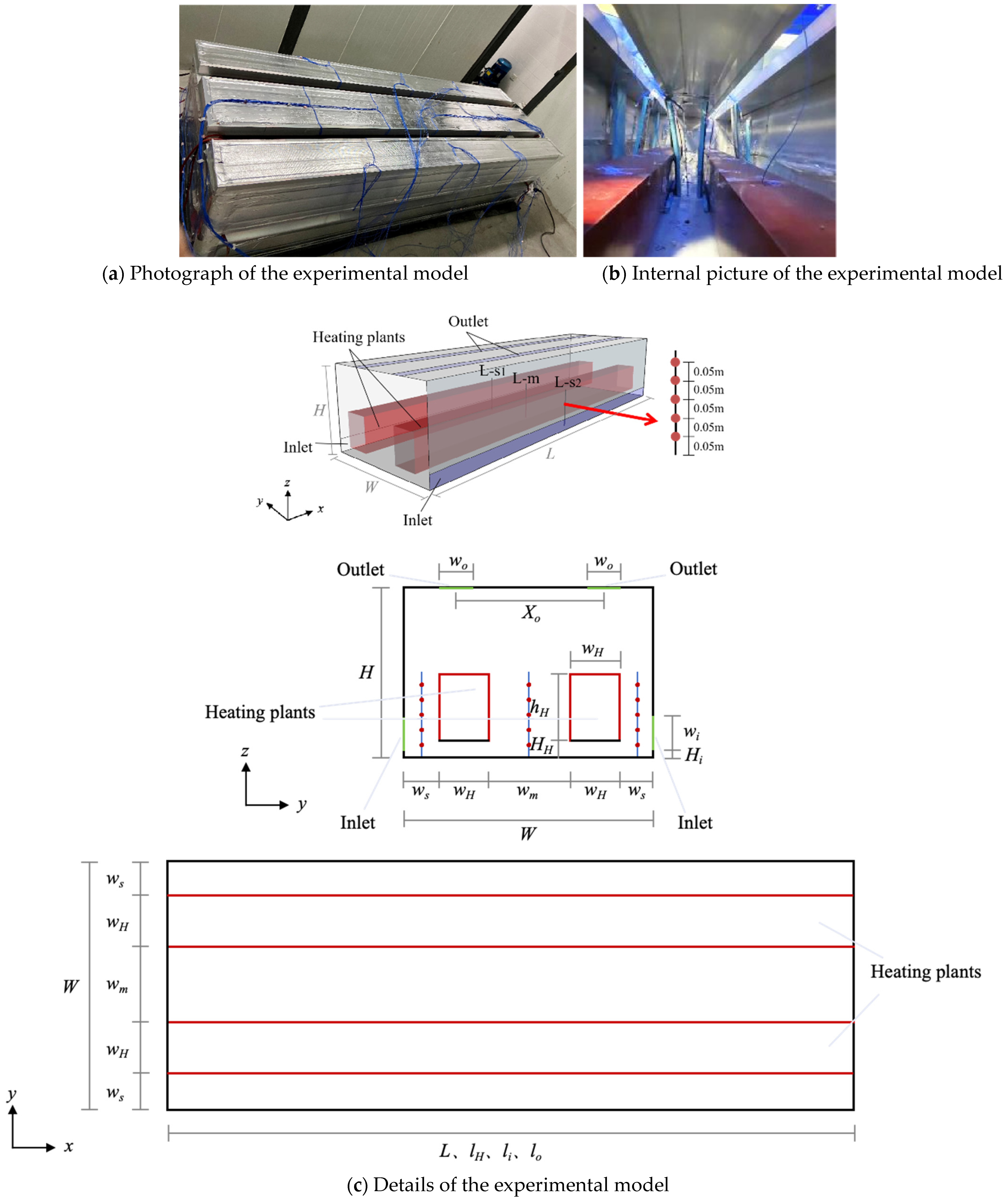
2.1. Scaled Experimental Model for Validation

Compared to conducting full-scale experiments, creating scaled experimental models can offer a flexible solution and save costs and time. For achieving similarity between the scaled model and the full-scale building, three aspects need to be considered: geometric, kinematic, and thermal similarities [32]. Geometric similarity can be easily achieved by uniformly scaling down the linear dimensions of the full-scale building in all three dimensions. In this study, a scaled model with a reduced scale of 1:20 has been developed (as illustrated in Figure 2) based on a naturally ventilated prototype building that was previously investigated in a thermal corridor workshop [21].

To ensure the validity of the results obtained from the scaled experimental model, a similarity analysis between the scaled model and the prototype building must be conducted. According to relevant research [33,34], the Reynolds number (Re) and Archimedes number (Ar) can be used as the similarity criterion. Indeed, achieving complete identity across all criteria besides the Prandtl number (Pr) is widely acknowledged as impractical. The Reynolds and Archimedes numbers are nonquantitative due to the uncertain velocity of free current [35]. Alternatively, the Grashof number (Gr) is an important scaling parameter combining these two numbers and characterizing the ratio of buoyancy to viscous forces; it is commonly used to analyze air flows with non-uniform density [36,37].

$$Gr=\frac{g\beta \Delta T{l}^3}{{\nu }^2}$$

(1)

where ν is the kinematic viscosity, m²·s⁻¹; g is the gravity acceleration, m·s⁻²; β is the thermal expansion coefficient, 1·K⁻¹; ∆T is the air temperature difference, K; and l is the characteristic height, m.

However, in practice, it is almost impossible to achieve an identical Grashof number between the scaled model and the prototype building [38]. Previous pieces of research [39,40] have suggested that the Grashof number’s critical value can be assumed to vary between 10⁶ and 10⁹, taking the room height into consideration as the characteristic height. In this study, with an experimental model height of 0.5 m and a temperature variation of 15 K to 95 K, the Grashof number for the scaled model falls within the range of 2.3 × 10⁸ to 8.3 × 10⁸. Therefore, for the buoyancy-driven ventilation model examined in this study the majority of the flow region can be viewed as Grashof number-independent. As a result, the turbulent viscosity can be utilized as a substitute for the Grashof number since it is proportional to both velocity and height [41].

$${\nu }_t\propto ul$$

(2)

$${\left(Gr\right)}_t\propto \frac{g\beta \Delta Tl}{u^2}$$

(3)

According to Lu et al. [35], the corresponding similarity conditions can be further described as Equation (4):

$$\frac{{\mathsf{\Pi }}_l·{\mathsf{\Pi }}_{\theta }}{{\mathsf{\Pi }}_u^2}=1$$

(4)

where ${\mathsf{\Pi }}_l$, ${\mathsf{\Pi }}_{\theta }$, and ${\mathsf{\Pi }}_u$ represent the contraction ratios for dimension, temperature, and velocity between the model and prototype. In most cases, ${\mathsf{\Pi }}_{\theta }$ = 1, implying T_R = T_F and ∆T_R = ∆T_F, the relationship simplifies to:

$$\frac{{\mathsf{\Pi }}_l}{{\mathsf{\Pi }}_u^2}=1$$

(5)

$$\frac{u_R}{u_F}={\left(\frac{l_R}{l_F}\right)}^{1/2}$$

(6)

where R refers to the reduced-scale model and F refers to the full-scale building; the model was developed with l_R/l_F = 1/20.

Figure 2 depicts the scaled building, and air is used as the working fluid. The enclosure structure comprised a metal sandwich plate; the ground was designed to be approximately adiabatic. The building model had dimensions of 2.5 m × 0.75 m × 0.5 m (length × width × height). There were two air inlets located at floor level along the façades, and two air outlets situated at the roof level. All these openings measured 2.5 m × 0.075 m (length × width). The heating plants were positioned 0.05 m above the floor level. The geometric conditions are summarized in

Table 1. Experimental model geometric parameters.

Name	Details
Dimensions of the experiment scaled-model, L × W × H	2.5 m × 0.75 m × 0.5 m
Dimensions of the heating plants, lH × wH × hH	2.5 m × 0.15 m × 0.2 m
Dimensions of the air openings, li × wi/lo × wo	2.5 m × 0.075 m
Width of the side corridor, ws	0.1 m
Width of the middle corridor, wm	0.25 m
Distance from the heating plants bottom to ground, HH	0.05 m
Distance from the inlet opening bottom to ground, Hi	0 m
Centre spacing of the outlet openings, Xo	0.325 m

.

Temperature measurement of the air was carried out using a K-type thermocouple and an Agilent 34980 data collector (Agilent Technologies, Santa Clara, CA, USA), with a measurement accuracy of ±0.5 °C and a time interval of 5 min. Nine thermal recorders were placed along a vertical axis, each positioned in the middle of the corridors, measuring temperatures within a height range of 0.05 m to 0.25 m, at 0.05 m intervals. The inlet and outlet opening velocities were determined using a Swema 3000 + SWA03 wind-speed probe, with a measurement accuracy of ±0.03 m/s and a time interval of 5 min.

Following the CFD validation, a parametric analysis is conducted to understand the impact of various geometric, heat transfer, and flow parameters on the convective heat transfer of the corridor. The variables considered in this paper include heating plant surface temperature, outdoor air temperature, heating plant sizes, air inlet and outlet sizes, and Rayleigh number. The simulation range for the variables considered is summarized in

Table 2. Variables examined in the CFD simulation.

Parameter	Range
Heating plants surface temperature, Tw	40–120 °C
Outdoor air temperature, T∞	21–31 °C
Air inlet/outlet area, Ai, Ao	0.125–0.2625 m2
Width of the heating plant, wH	0.1–0.3 m
Height of the heating plants, hH	0.05–0.175 m
Rayleigh number, Ra	4 × 106, 4 × 107

.

2.2. Governing Equations

The commercial software ANSYS Fluent (version 17.0) was employed to conduct the CFD simulation. To simplify the calculation process, the CFD simulation assumes three-dimensional, constant fluid properties, fully turbulent, incompressible flow, and steady flow, neglecting viscous dissipation. The equations describing air velocity and temperature in three dimensions under steady-state conditions, assuming constant thermal properties, incompressibility, and non-viscous dissipation, can be expressed as follows [42,43].

Continuity equation:

$$\frac{\partial \left(\rho u_i\right)}{\partial x_i}=0$$

(7)

Momentum equation:

$$\frac{\partial \left(\rho u_i{u}_j\right)}{\partial x_i}=-\frac{\partial \mathsf{\rho }}{\partial x_j}+\frac{\partial }{\partial x_j}\left(\mu \left(\frac{\partial u_i}{\partial x_j}+\frac{\partial u_j}{\partial x_i}\right)-\rho \overline{u_I^{\prime }{u}_J^{\prime }}\right)+\rho \beta \left(T-T_0\right)g_i$$

(8)

Energy equation:

$$\frac{\partial \left(\rho u_{i}T\right)}{\partial x_i}=\frac{1}{c_p}\frac{\partial }{\partial x_j}\left(\lambda \frac{\partial \mathrm{T}}{\partial x_i}\right)+\frac{\partial }{\partial x_j}\left(-\rho \overline{u_J^{\prime }T}\right)$$

(9)

where T₀, $\beta$, and $\overline{u_J^{\prime }T}$ represent the operation temperature, thermal expansion coefficient, and turbulent heat flux, respectively. The constant values for various governing equations can be determined using these expressions [44].

The realizable k-ε model was selected for all sets of simulations in this study for better simulation results under high-temperature buoyant effects conditions [45]. The air is treated as incompressible, with density variation effects addressed through the Boussinesq approximation [46]. Consideration radiation effects, the air was assumed to be transparent to radiation [47]. The surface-to-surface (S2S) radiation model, which relies on the view factor affected by size, distance, and orientation [48], was applied in this study to calculate radiative heat transfer.

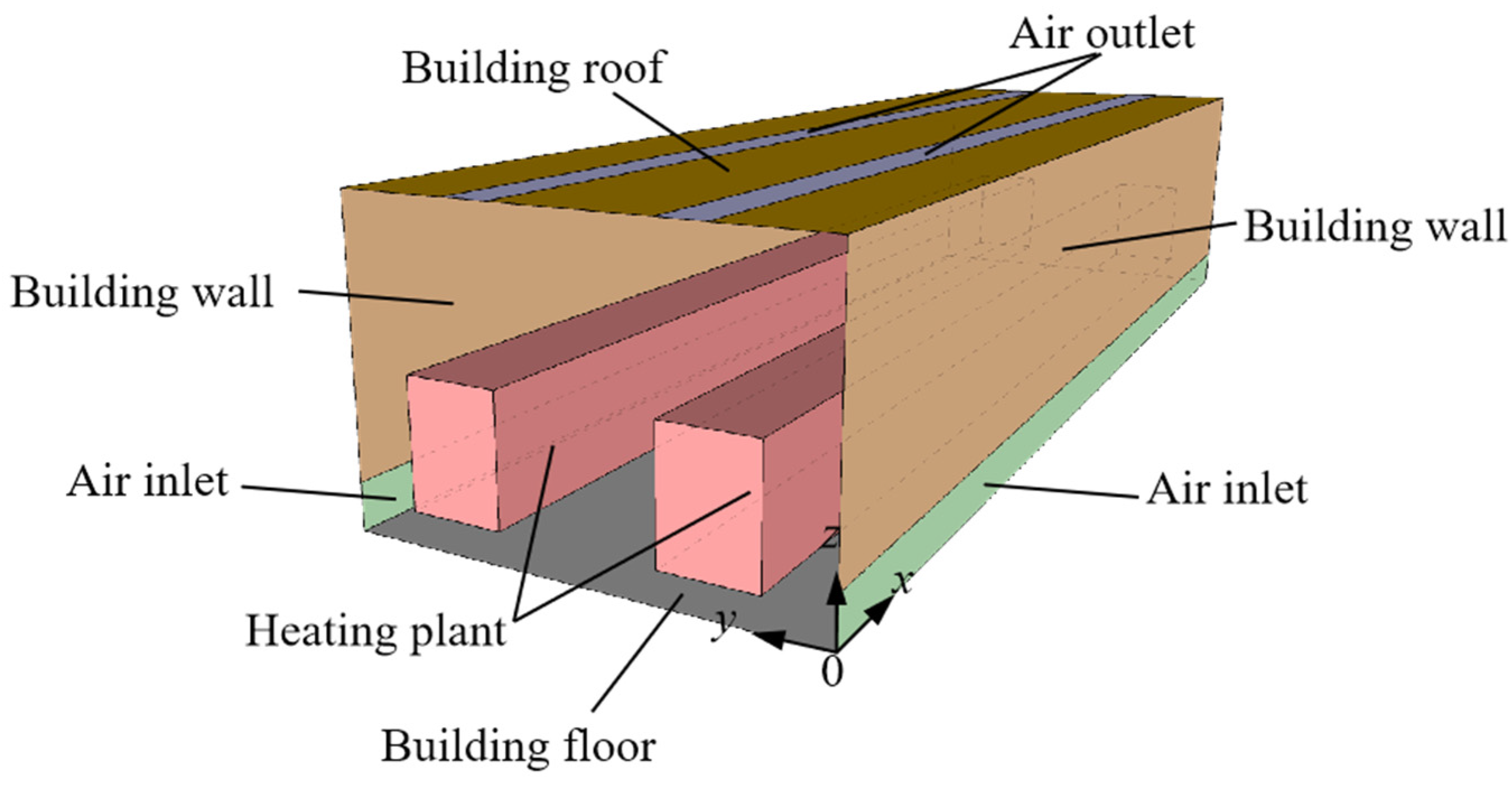
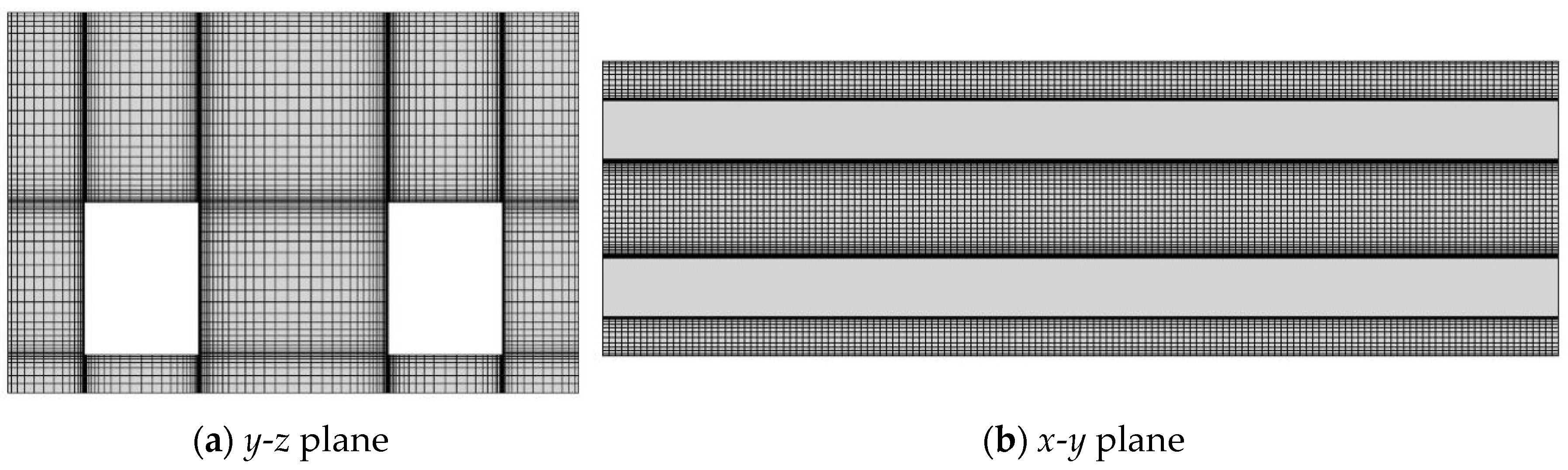
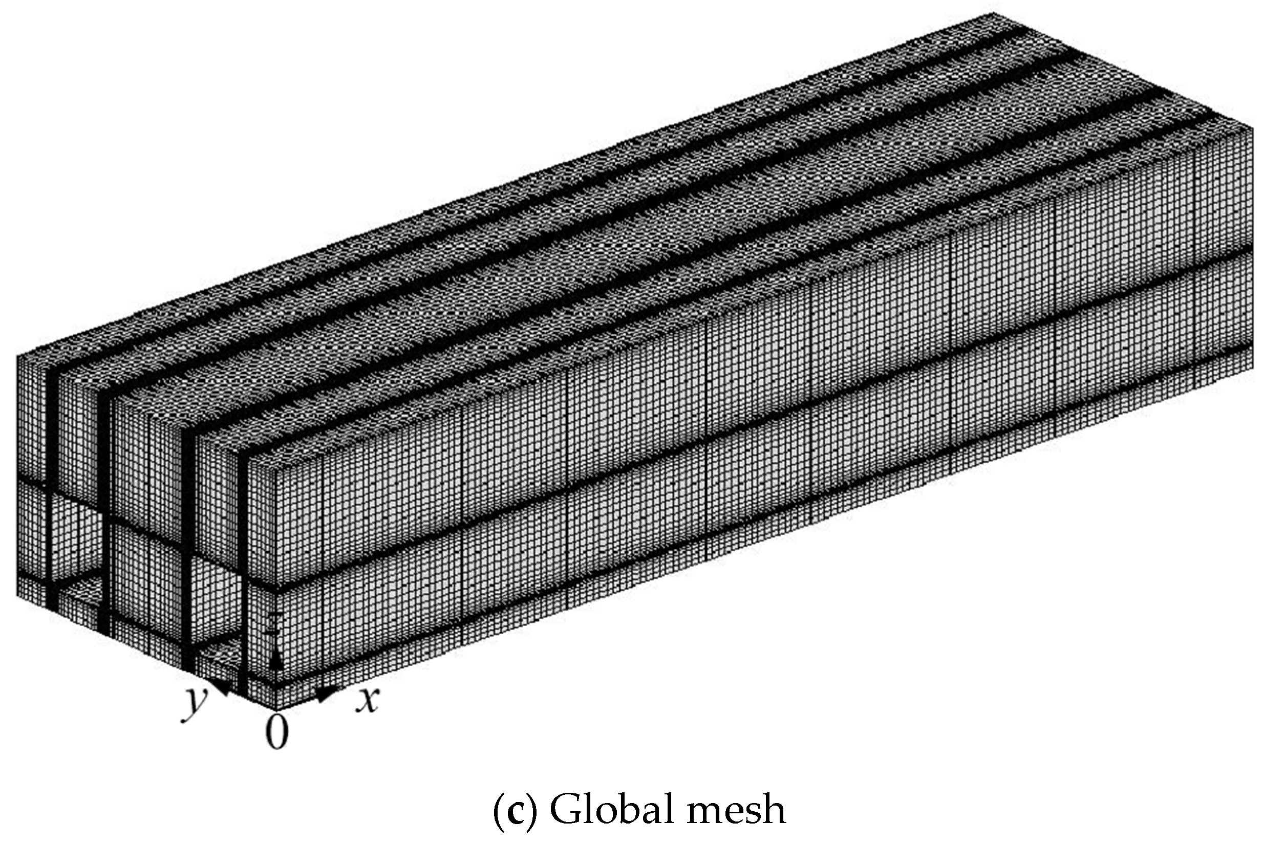
2.3. Computational Grids and Boundary Conditions

Figure 3 displays the computational domain, which corresponds to the experimental model geometry. To precisely depict the natural convection in thermal corridors, an enhanced wall treatment approach, which merges a two-layer model with enhanced wall functions, is utilized. For accurate simulation of the near-wall region, it is important to ensure that the dimensionless wall distance, y+, is close to 1 [49]. To achieve this, a high cell density is required in the near-wall region. The mesh employed for this study was generated using ICEM CFD 15.0 software. Structured mesh elements are employed to discretize the entire computational domain, as depicted in Figure 4. The grid is refined in proximity to the heating plants and air openings to capture significant gradients in this area.

The grid-independent test is crucial in numerical simulations to ensure that the results are not sensitive to changes in mesh size. The test is performed based on the dimensionless axial temperature along the middle corridor by varying grid sizes from 0.42 million to 0.95 million, as shown in Figure 5. The dimensionless temperature is expressed as:

$$\theta =\frac{T-T_{\infty }}{T_w-T_{\infty }}$$

(10)

where T is the measured air temperature of the corridor, °C; T_w is the surface temperature of heating plants, °C; and T_∞ is the outdoor air temperature, °C.

The results demonstrate that as the number of mesh elements increases from 0.42 million to 0.74 million, there is a significant fluctuation in air temperature. The mesh number increases from 0.74 million to 0.95 million, and the percentage error is below 5%. As a result, a mesh comprising 0.74 million elements was preferred for simulation, which can reduce computing time and maintain simulation accuracy. The minimum and maximum grid sizes are 0.9 mm and 17 mm, respectively, with a growth rate not exceeding 1.2. In the near-wall region, the surface-averaged y+ is around 1 and the maximum value is below 3.

Table 3. Boundary conditions.

Description of the Area	Type	Boundary Conditions
Building walls and roof	Wall	Overall heat transfer coefficient: 0.8 W/(m2·K), heat transfer coefficient in the outer surface of the walls: 20.9 W/(m2·K), temperature: 25 °C, emissivity: 0.85
Building floor	Wall	Adiabatic
Heating plant (top and side)	Wall	Temperature: 80 °C, emissivity: 0.85
Air inlet	Pressure inlet	Temperature: 25 °C, pressure: 0 Pa
Air outlet	Pressure outlet	Temperature: 25 °C, pressure: 0 Pa

summarizes the boundary conditions of the CFD model used in the simulation. The solid surfaces were assumed to have a no-slip condition, while the floor of the workshop and the bottom of the heating plants were set to be adiabatic. As for the workshop’s ceiling and side walls, the convection boundary type was utilized along with the heat transfer coefficient and ambient temperature boundary conditions [50]. The overall heat transfer coefficient is 0.8 W/(m²·K), and the heat transfer coefficient on the outer surface of the walls is 20.9 W/(m²·K) [51]. A constant wall temperature was applied to the top and side surfaces of the heating plants. Heat transfer due to radiation was accounted for using a constant emissivity value of 0.85 [46,52,53]. Initially, the outdoor air temperature was set at 25 °C and the heating plant temperature at 80 °C. For modelling the buoyancy-driven flow within the corridor, all inlet and outlet openings were designated as pressure inlet and outlet [54], respectively, with their values set at 0 Pa.

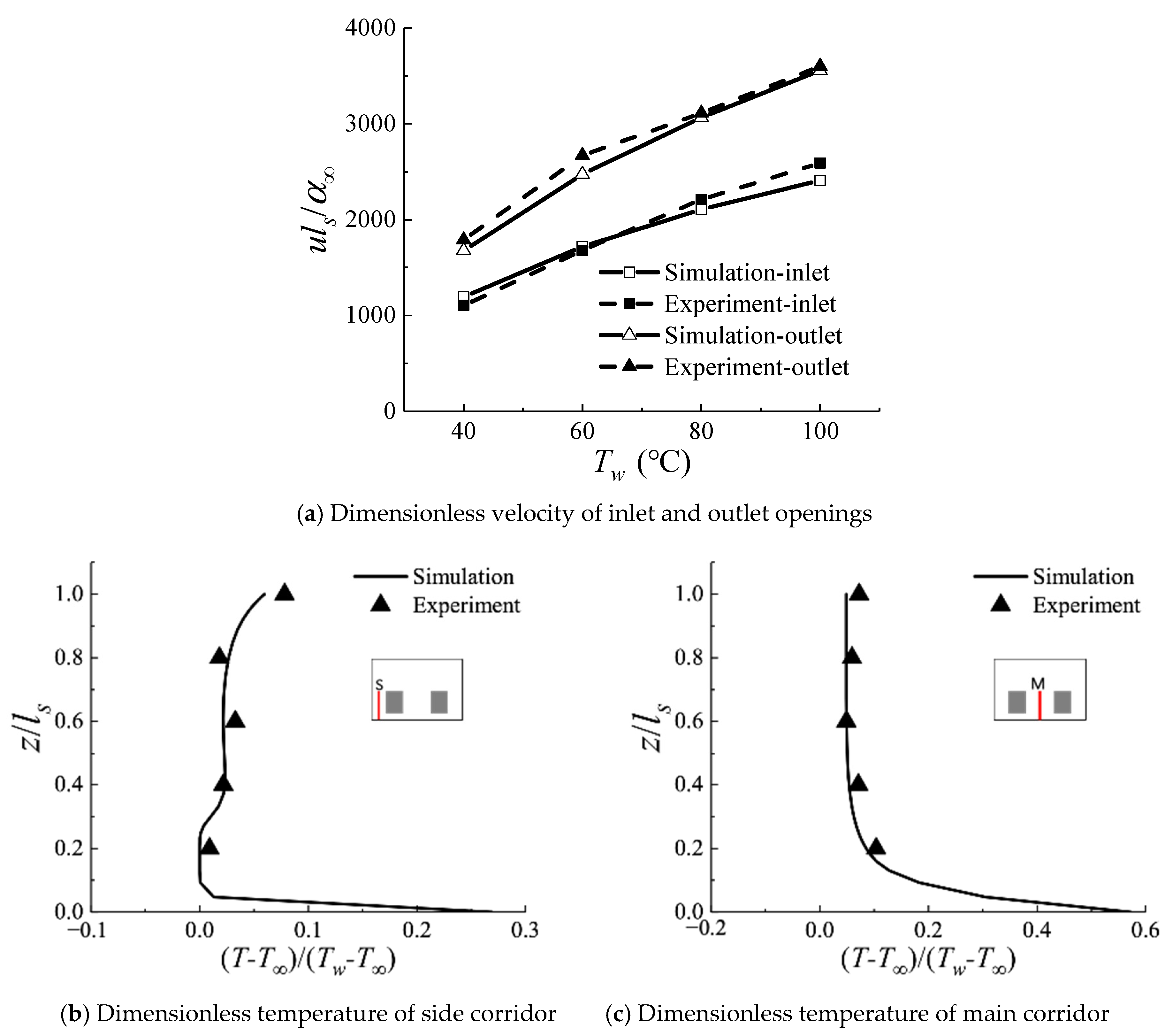
2.4. Solver Schemes and Model Validation

Pressure interpolation was achieved using the QUCK scheme, and the SIMPLE algorithm was employed to handle the velocity–pressure coupling [55]. The energy, momentum, k, and ε equations were all calculated using a second-order upwind scheme [56]. The pressure term was discretized using the Body Force Weighted algorithm. The numerical solutions were considered to be converged when the relative residual of energy was not greater than 10⁻⁶ and the relative residual of the two iterations of variables were lower than 10⁻³ [57].

Simulation results were compared with the experimental data to validate the numerical model using dimensionless velocity and dimensionless temperature (Equation (10)). The dimensionless velocity is expressed as:

$$U=\frac{ul}{{\alpha }_{\infty }}$$

(11)

where u is the measured air velocity, m·s⁻¹; l is the channel height, m; and α_∞ is the thermal diffusivity, m²·s⁻¹.

As illustrated in Figure 6a, increasing the heating plants’ temperature led to an increase in both inlet and outlet dimensionless velocities. Moreover, the dimensionless velocity at the outlet was consistently greater than at the inlet. Figure 6b,c shows the vertical dimensionless temperature of the side corridor fluctuates slightly, with lower temperature at the bottom and higher temperature in the upper area. The vertical dimensionless temperature of the middle corridor is more stable and basically constant. In general, the side corridor temperature is lower than the middle corridor temperature. The maximum relative errors for dimensionless velocity and dimensionless temperature are 8.1% and 4.5%, respectively. The discrepancies may stem from experimental errors, particularly in heat generation [43]. Despite implementing protective measures, thermocouple measurements can be affected by radiative exchanges with the ambient environment when used in high-temperature heat sources, with an error of up to 1% within the temperature range from 20 to 200 °C [58].

In our simulation validation, dimensionless velocity and dimensionless temperature are not directly measured but derived as functions of other directly measured variables. Each measured variable demonstrates random variability, referred to as “uncertainty”, for each device. To assess the uncertainty of the calculated data due to error propagation, we utilized the method introduced by Zhang et al. [59]. The following equation is used to determine the uncertainty of the calculated parameters:

$$U_Y^2={\sum }_i{\left(\frac{\partial Y}{\partial X_i}\right)}^2{U}_{X_i}^2$$

(12)

Here, U_Y is the uncertainty associated with the variable Y and U_Xi are the uncertainties associated with each measured variable X_i. Assuming constant thermophysical properties, the resulting uncertainties associated with dimensionless velocity and dimensionless temperature measurements were ±4.65% and ±3.96%, respectively. Overall, the variance between the measured and simulated values in the corridor is not extremely high and could be deemed acceptable.

3. Results and Discussion

3.1. Temperature and Velocity Distribution Investigations

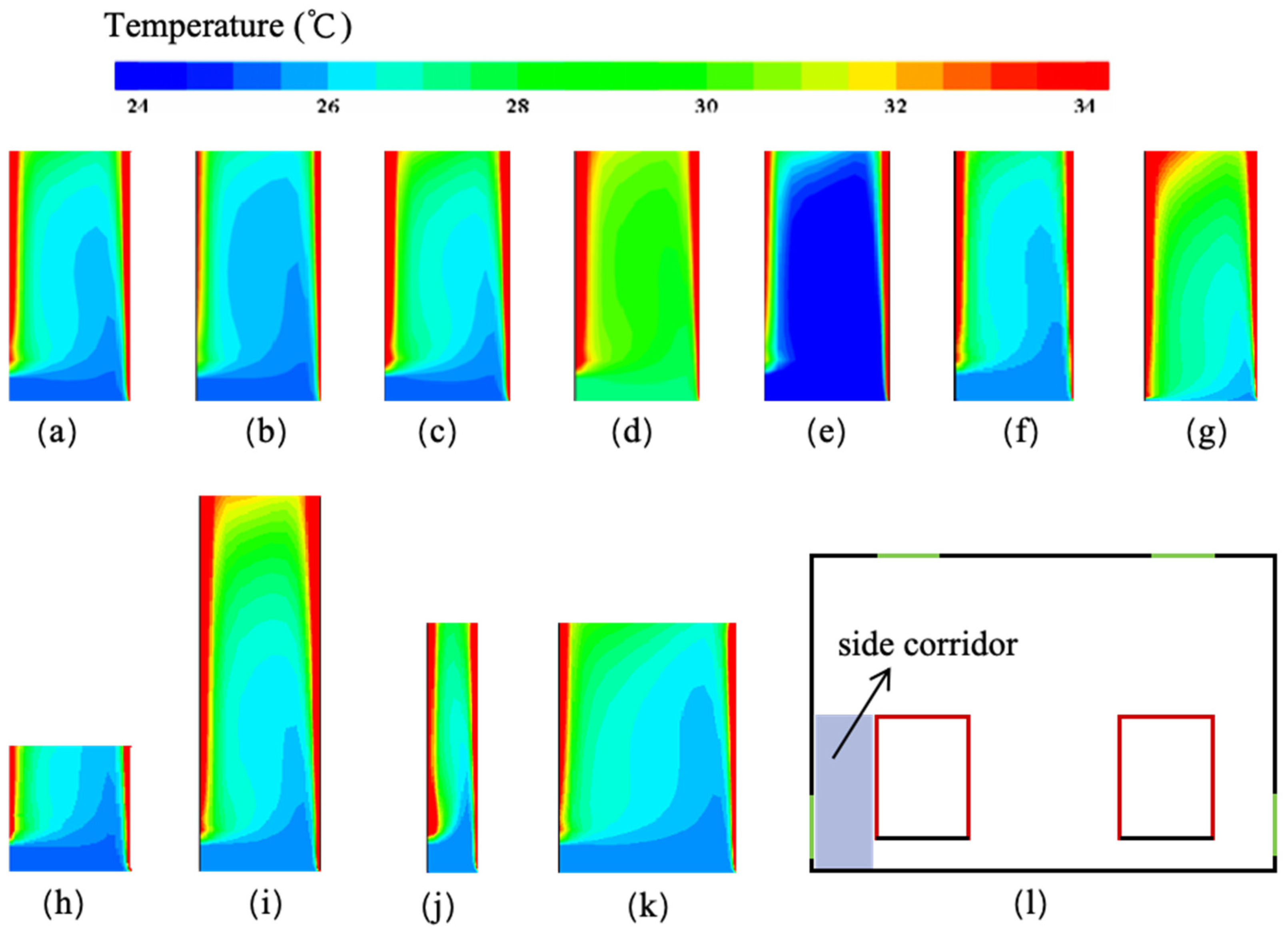
3.1.1. Side Corridor

To visualize the effect of different parameters on thermal fields, Figure 7 shows isotherms plotted at various conditions. Given that indoor temperature control targets for industrial buildings usually do not exceed 35 °C, we have set the temperature legend to this maximum value. Figure 7a–c illustrate the thermal contours inside the corridor for different surface temperatures of the heating plant. It van be observed that the heating plant temperature mainly influences the air temperature in the middle-upper area, while the lower working area remains close to the air inlet. When the surface temperature of the heating plants is increased from 60 to 100 °C, the air temperature in the side corridor increases by approximately 1 °C. In Figure 7a,d,e, the ambient air temperature shows a significant impact on the temperature distribution of the entire corridor. Increasing the ambient air temperature of the inlet from 22 to 28 °C results in a substantial increase in the side corridor temperature, by approximately 6 °C. Figure 7a,f,g compare the geometry of the inlet and outlet, showing that the size of the outlet has less effect on the temperature distribution of the side corridor, with only a 1 °C temperature difference. However, when the outlet size is constant and the inlet size drops by 30%, the air temperature in the side corridor increases by 3 °C. Figure 7a,h–k describe a comparison of the geometry of the heating plants, demonstrating how the waste heat in the corridor changes with the size of the heating plants. Additionally, it can be noted that when the height of the corridor increases, hot air cannot be easily discharged, which can reduce the efficiency of the buoyancy ventilation system.

The velocity patterns obtained with different parameters are presented in Figure 8. The velocity at the location of the inlet and near the wall of the heat source is approximately four times higher than in other locations within the corridor. This indicates localized areas of higher airflow. Figure 8a–c demonstrate that the temperature of the heat source mainly affects the inlet velocity of the side corridor and the airflow velocity near the wall of the heat source. Similarly, the ambient air temperature exhibits a similar trend. With the decrease of inlet size, the velocity of the main flow in the side corridor increases significantly. Figure 8a,h–k imply that reducing the heating plant height weakens the total heat transfer in the corridor, leading to a decrease in flow velocity. As the corridor widens, the descending flow increases, and the flow can be trapped by a return flow and zone of depression. The flow pattern of the side corridor, which can be seen as a heated asymmetric channel, is summarized in Figure 9.

The velocity and temperature profiles within the asymmetric corridor are notably influenced by varying the Rayleigh number (Ra). For this study, two different Rayleigh numbers were investigated using the numerical model, with A_o/A_i = 1 and l_s/w_s = 2, at different sections of the side corridor, z/l_s = 0%, 25%, 50%, 75%, and 100%. Figure 10 and Figure 11 display the dimensionless temperature and velocity at various y/w_s, beginning at y/w_s = 0 for the cold wall and ending at y/w_s = 1 for the heated wall.

With an increase in Rayleigh number, a fully developed heat transfer flow at the export is assumed, and the corridor exit temperature reaches its maximum. The lower Rayleigh number corresponds to lower air temperatures in the side corridor. From the inlet towards the downstream of the corridor, the peak velocity value increases gradually. In the central mainstream area of the side corridor (y/w_s = 0.2–0.85), apparently the lower Raleigh number has the faster flow speed; and under the same Ra circumstances the velocity values decrease with an increase in position height.

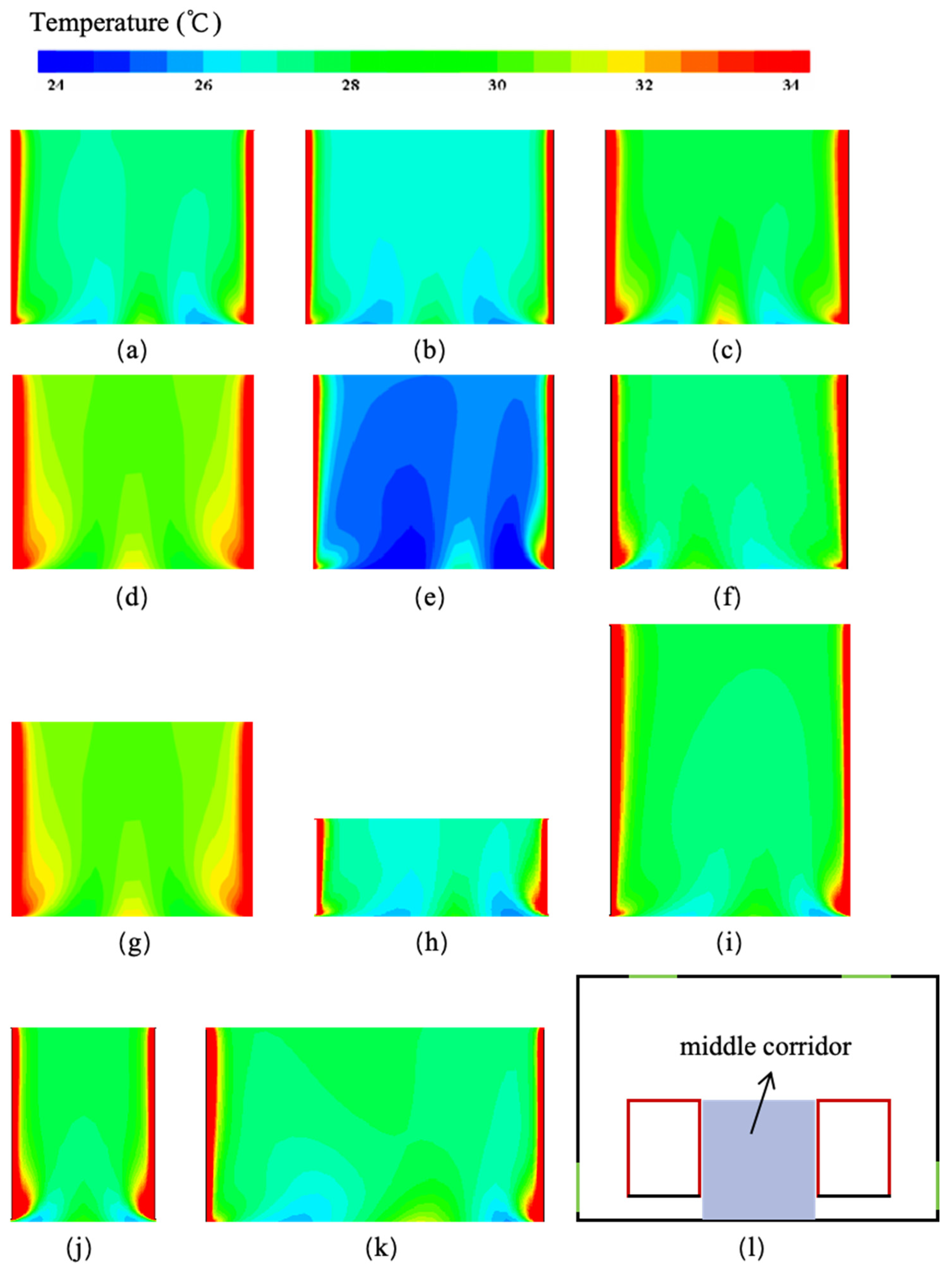
3.1.2. Middle Corridor

Figure 12 presents the temperature distributions in the middle corridor for various parameters, such as temperature, air opening size, and heating plants geometry. The air within the middle corridor exhibits a more stable, elevated temperature relative to that present in the side corridor. As shown in Figure 12a–c, when the surface temperature of the heating plants is increased from 60 to 100 °C, the air temperature in the middle corridor increases by approximately 2 °C. However, when the ambient air temperature of the inlet is increased from 22 to 28 °C, there is a substantial increase in middle corridor temperature, by approximately 7 °C. When the inlet size is kept constant and the outlet size drops by 30%, the air temperature in the middle corridor increases slightly. Conversely, when the outlet size is constant and the inlet size drops by 30%, the air temperature in the middle corridor increases by 3 °C. Comparing the effect of heating plant geometry on corridor temperature, it can be observed that different sizes of heating plants result in a small variation in corridor temperature, with changes of no more than 2 °C.

Figure 13 provides insight into the streamlines and velocity fields under various parameters. Notably, the overall velocity difference in the middle corridor appears smaller compared to that in the side corridors, indicating relatively uniform airflow. The air velocity in the middle corridor seems primarily influenced by outdoor temperature, with other parameters having a lesser impact. Theoretically, the temperature and velocity distributions in the middle corridor should be symmetric under symmetrical parameter arrangements. However, deviations from this expected outcome can occur, particularly when the outdoor temperature is lower. This phenomenon is often observed in steady natural convection flows in a horizontal channel containing isothermal heating rectangular blocks [60,61,62]. When the Rayleigh number (Ra) changes, the flow regime becomes unsteady, characterized by sustained periodic oscillations. An increase in Ra to a certain extent can indeed lead to dissymmetrical flow patterns. Ideally, the flow pattern of the middle corridor, resembling a heated symmetric channel, is succinctly summarized in Figure 14. In configurations with symmetric heating plants, the streamlines remain parallel to the wall, suggesting fully developed flow within the central zone.

The current numerical simulation was conducted for two Raleigh numbers, with A_o/A_i = 1 and l_s/w_s = 2 at different sections of the middle corridor, z/l_s = 0%, 25%, 50%, 75%, and 100%. Temperature and velocity profiles are illustrated in Figure 15 and Figure 16. The temperature profiles become mainly horizontal and reach a minimum value at y/w_m = 0.4–0.6, indicating that the working zone should be set up in this area for better thermal comfort effect. For high Raleigh numbers, the temperature profiles become more uniform, indicating that the flow inside the corridor is stable. Figure 16b indicates the peak velocity for high Raleigh numbers is much higher. The conclusion is consistent with the low Raleigh number case (Ra = 4 × 10⁶), but at high Raleigh numbers (Ra = 4 × 10⁷) the fluid starts to become disturbed and disorderly.

3.2. Correlations for Heat Transfer and Flow Prediction

3.2.1. Side Channel

Based on the results of the simulations, the natural convection characteristics of the side corridor are quite like those of vertical heated channels. As a result, this section presents the semi-empirical correlations for both the average wall heat transfer, ${\overline{Nu}}_s$, and induced mass flow rate, ${\dot{m}}_s$, of the side channel. Figure 17 depicts a schematic of the problem.

The side channel was composed of one exterior wall and one isothermal vertical heating plate, with height, l, spaced at a distance, w_s. Several parameters were considered: the channel size, the inlet vents size, and the characteristic temperature. Since air does not act as an absorptive or emitting medium for the temperature range, radiation loss was calculated separately.

To generate generalizable heat transfer results, the surface-averaged Nusselt number along the heated wall is defined as follows:

$${\overline{Nu}}_s=\frac{h_{s}l}{\lambda }$$

(13)

$$h_s=\frac{q_{cv,s}}{T_w-T_{\infty }}$$

(14)

where q_cv,s is the heat flux of convective heat transfer in the side channel, W·m⁻²; h_s is the convective heat transfer coefficient, W·m⁻²·°C⁻¹; T_w and T_∞ are the heated plates temperature and ambient air temperature, respectively, °C.

In free-convection flow, the buoyant potential is balanced by the buoyant potential expressible as

$$\frac{dP}{dx}{\mid }_{buoy}=\left({\rho }_f-{\rho }_{\infty }\right)g=-\rho \beta g\left(T_f-T_{\infty }\right)$$

(15)

An energy balance is attained when the heat transferred from the isothermal wall is equal to that absorbed in the flow, which can be expressed as follows:

$${\dot{m}}_s{c}_{p}l\left(T_f-T_{\infty }\right)=h_s\left(T_w-T_f\right)$$

(16)

where ${\dot{m}}_s$ is the flow rate in the side channel, kg·(m·s)⁻¹; T_f is the fluid temperature of the side channel, °C.

Previous studies [26,28,30,31,63,64,65] on natural convective characteristics have clarified that the surface-averaged Nusselt number can be expressed using the formula ‘Raⁿ’ + dimensionless. Additionally, formulas for the flow rate can be constructed using the formula ‘Ra^N × Pr^M’ + dimensionless coefficients, as depicted below:

$$Nu=c{\left(Ra\right)}^n$$

(17)

$$\dot{m}=C{\left(Ra\right)}^{N}P{r}^M$$

(18)

where $Ra=Gr·Pr$, $Gr=\frac{g\beta △T{l}^3}{{\upsilon }^2}=\frac{g\beta \left(T_w-T_{\infty }\right)l^3}{{\upsilon }^2}$, $Pr=\frac{v}{\alpha }$.

To evaluate the influence of channel aspect ratio, w_s/l, on the results, for the uniform wall temperature the following Rayleigh number is used:

$${R{a}_s}^{*}=R{a}_s\cdot \left(w_s/l\right)=\frac{g\beta \left(T_w-T_{\infty }\right)l^3\left(w_s/l\right)}{\alpha \nu }$$

(19)

Thus, the empirically correlation of Nusselt number and induced mass flow rate for the side channel can be estimated from

$${\overline{Nu}}_s=a_1{\left(\frac{A_i}{A_o}\right)}^{b_1}{\left(R{a}_s^{*}\right)}^{c_1}$$

(20)

$${\dot{m}}_s=a_2{\left(\frac{A_i}{A_o}\right)}^{b_2}{\left(R{a}_s^{*}\right)}^{c_2}P{r}^{d_2}$$

(21)

In these two equations, the values of a₁, b₁, c₁, a₂, b₂, c₂, and d₂ can be determined by fitting the data extracted from simulation results. Following this idea, it can be proposed for ${\overline{Nu}}_s$ (for 3.6 × 10⁶ ≤ Ra_s* ≤ 3.4 × 10⁷):

$${\overline{Nu}}_s=0.7627{\left(\frac{A_i}{A_o}\right)}^{-0.0383}{\left(R{a}_s^{*}\right)}^{0.25}$$

(22)

For ${\dot{m}}_s$, the following correlations can be proposed:

When A_i/A_o < 1:

$${\dot{m}}_s=0.00356{\left(\frac{A_i}{A_o}\right)}^{0.3397}{\left(R{a}_s^{*}\right)}^{0.2}P{r}^{0.3}$$

(23)

When A_i/A_o > 1:

$${\dot{m}}_s=0.00158{\left(\frac{A_i}{A_o}\right)}^{-0.3126}{\left(R{a}_s^{*}\right)}^{0.25}P{r}^{0.3}$$

(24)

When A_i/A_o = 1:

$$\dot{m_s}=5.2165\times {10}^{-7}{\left({Ra}_s^{*}\right)}^{0.7245}{Pr}^{0.3}$$

(25)

The application scope of the mentioned correlations (Equations (22)–(25)) is limited by the followings: 0.5 ≤ A_i/A_o ≤ 4.0, 3.6 × 10⁶ ≤ Ra_s* ≤ 3.4 × 10⁷. With the same set of parameters, the surface-averaged ${\overline{Nu}}_s$ and induced flow rate, ${\dot{m}}_s$, from correlations together with the simulation data are compared in Figure 18.

Figure 18 compares the surface-averaged and induced mass flow rate from the semi-empirical correlations with the simulation data for the side channel. The comparison shows good agreement, with relative errors from the correlations being less than 5% in most cases and the maximum relative deviation being less than 10%. The maximum relative deviation is 12%. Therefore, these correlations can be reliably used to describe convective exchange in the side channel under their validity conditions.

3.2.2. Middle Channel

Similarly, the semi-empirical correlations for surface-averaged ${\overline{Nu}}_m$ and induced mass flow rate, ${\dot{m}}_m$, of the middle channel are concluded in this section. Figure 19 depicts a schematic of the problem. The middle channel consists of two isothermal vertical heating plates with a height l, situated at a distance of w_m from each other.

Referring to the previous work of the side channel, the energy balance can be expressed as

$${\dot{m}}_m{c}_{p}l\left(T_f-T_{\infty }\right)=2h_m\left(T_w-T_f\right)$$

(26)

where ${\dot{m}}_m$ is the flow rate in the middle channel, kg·(m·s)⁻¹; h_m is convective heat transfer coefficient of middle channel, W·m⁻²·°C⁻¹.

Like side channel, the empirical correlation of Nusselt number and induced flow rate for the middle channel can be estimated from

$${\overline{Nu}}_m=a_3{\left(\frac{A_i}{A_o}\right)}^{b_3}{\left(R{a}_m^{*}\right)}^{c_3}$$

(27)

$${\dot{m}}_m=a_4{\left(\frac{A_i}{A_o}\right)}^{b_4}{\left(R{a}_m^{*}\right)}^{c_4}P{r}^{d_4}$$

(28)

where $R{a}_m^{*}=R{a}_m\cdot \left(w_m/l\right)=\frac{g\beta \left(T_w-T_{\infty }\right)l^3\left(w_m/l\right)}{\alpha \nu }$.

In these two equations, the values of a₃, b₃, c₃, a₄, b₄, c₄, and d₄ can be determined by fitting the data extracted from simulation results. Following this idea, the following can be proposed for ${\overline{Nu}}_m$ (for 3.6 × 10⁶ ≤ Ra_m* ≤ 3.4 × 10⁷):

$${\overline{Nu}}_m=0.4737{\left(\frac{A_i}{A_o}\right)}^{0.0056}{\left(R{a}_m^{*}\right)}^{0.25}$$

(29)

For ${\dot{m}}_m$, the following correlations can be proposed:

When A_i/A_o ≠ 1:

$${\dot{m}}_m=0.00344{\left(\frac{A_i}{A_o}\right)}^{-0.2968}{\left(R{a}_m^{*}\right)}^{0.245}P{r}^{0.3}$$

(30)

When A_i/A_o = 1:

$$\dot{m_m}=0.3702\times {10}^{-9}{\left({Ra}_m^{*}\right)}^{1.1677}{Pr}^{0.3}$$

(31)

The application scope of the mentioned correlations (Equations (29)–(31)) is limited by the followings: 0.5 ≤ A_i/A_o ≤ 4.0, 3.6 × 10⁶ ≤ Ra_m* ≤ 3.4 × 10⁷. Using the same set of parameters, a comparison is conducted between the simulations and correlations.

Figure 20 displays a comparison between the surface-averaged ${\overline{Nu}}_m$ and induced flow rate, ${\dot{m}}_m$, obtained from the semi-empirical correlations and numerical simulation data. The figures demonstrate good agreement between the correlations and the numerical results. In most cases, the relative errors of ${\overline{Nu}}_m$ from semi-empirical correlations are less than 5% and the maximum relative devotion is less than 10%. Additionally, the relative errors of ${\dot{m}}_m$ from semi-empirical correlations are less than 10% and the maximum relative devotion is less than 16%. It can be seen that when A_i/A_o > 1 is greater than 1, the accuracy of flow rate prediction may be compromised due to its strong dependence on the inlet area, particularly when the inlet area significantly exceeds the outlet area. However, over 80% of the predicted results have an error within 15%, which closely aligns with the fitting results of relevant studies [66,67] and is considered acceptable. Therefore, within their validity conditions these correlations can correctly describe the convective exchange in channel.

4. Conclusions

The understanding of flow and heat exchange patterns in natural convection within thermal corridors remains unclear. This paper addresses this gap by investigating the natural convection characteristics of air on vertical plates within industrial building corridors, under both symmetric and asymmetric heating conditions. The goal is to improve the thermal environment within and around these corridors, thereby aiding in the design of industrial buildings equipped with buoyancy-driven ventilation systems.

(1)

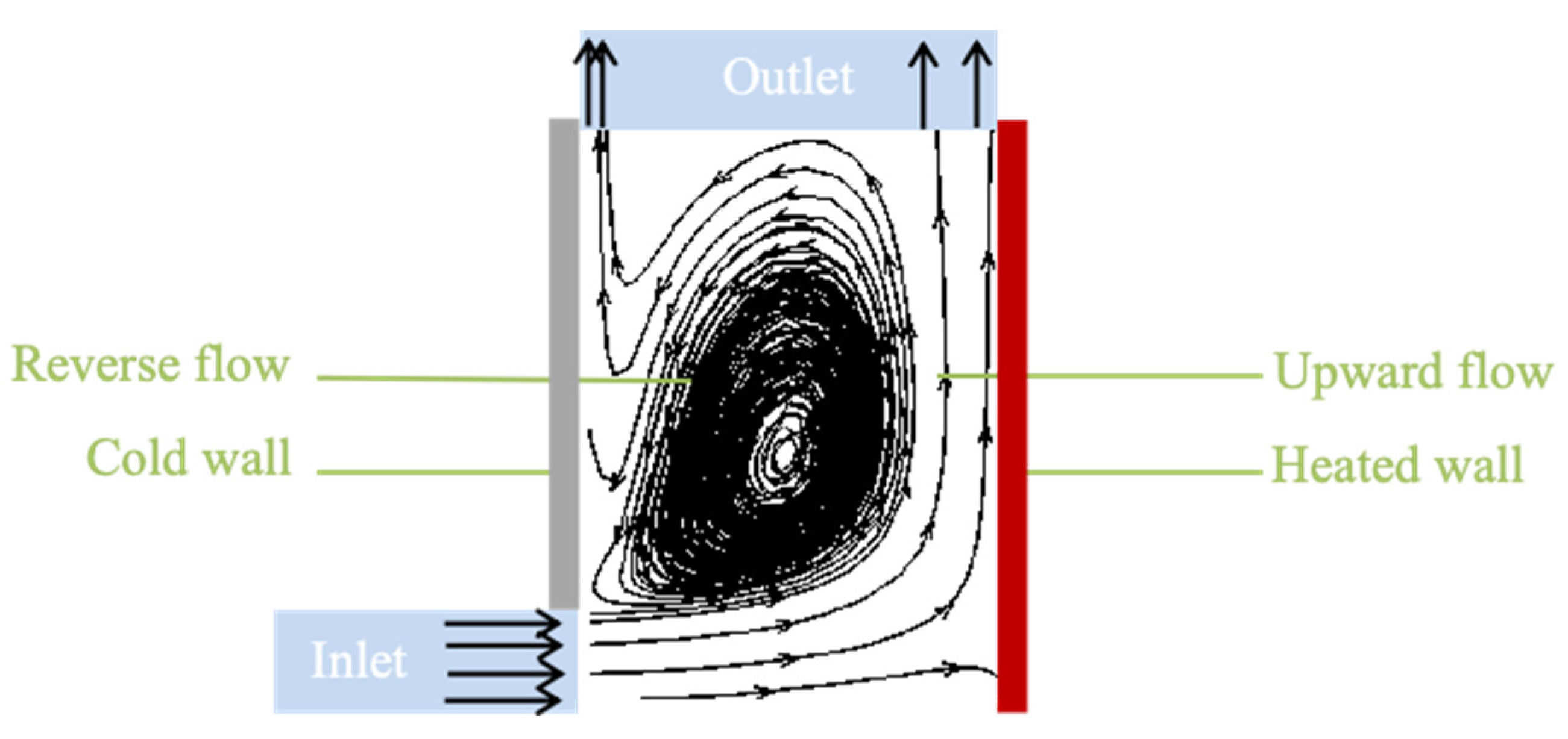
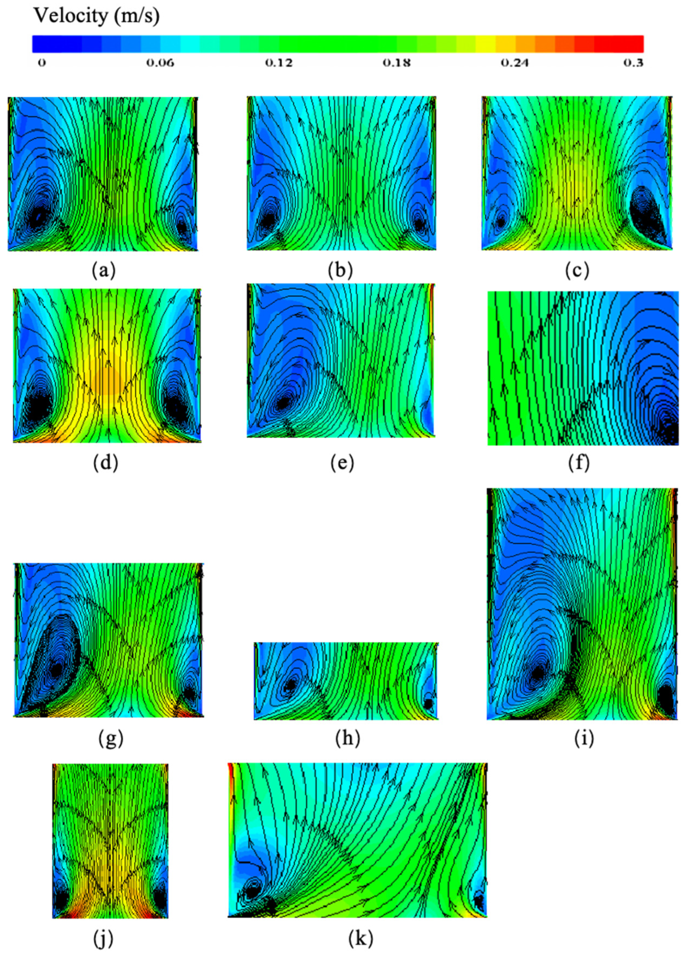
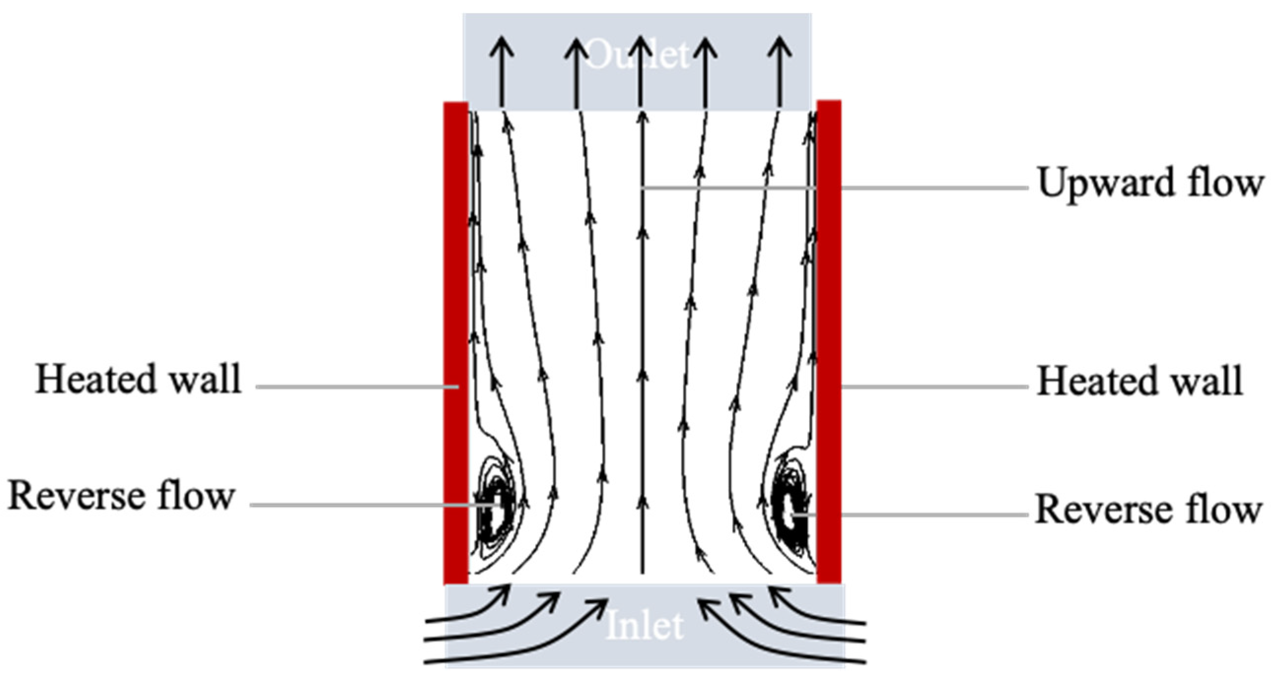
In the side corridor, the prevalence of reverse flow dominates much of the channel, leading to an uncomfortable thermal environment within the working zone. The ambient air temperature significantly influences the temperature distribution throughout the entire corridor. Increasing the ambient air temperature at the inlet from 22 to 28 °C results in a substantial temperature rise in the side corridor, by approximately 6 °C.

(2)

In the middle corridor, the occurrence of reverse flow near the bottom corner is noted, while the air within the middle corridor exhibits a more stable yet elevated air temperature. The ambient air temperature at the inlet plays a significant role in the middle corridor’s thermal environment, while the surface temperature of the heating plants has a lesser impact. When the outlet size remains constant and the inlet size decreases by 30%, the air temperature in the middle corridor increases by 3 °C.

(3)

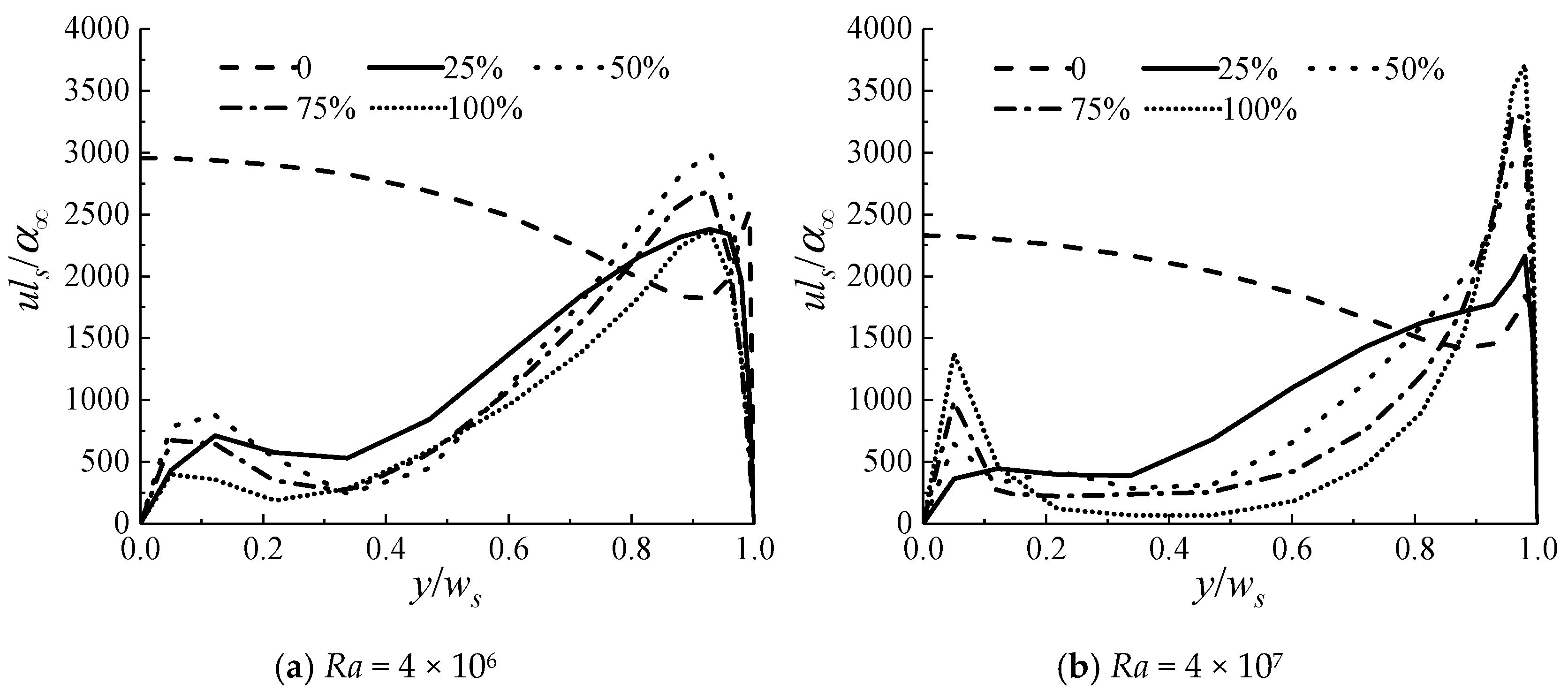
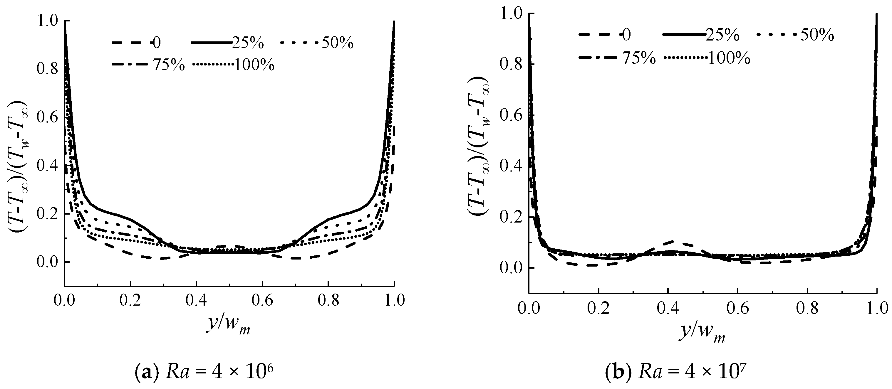
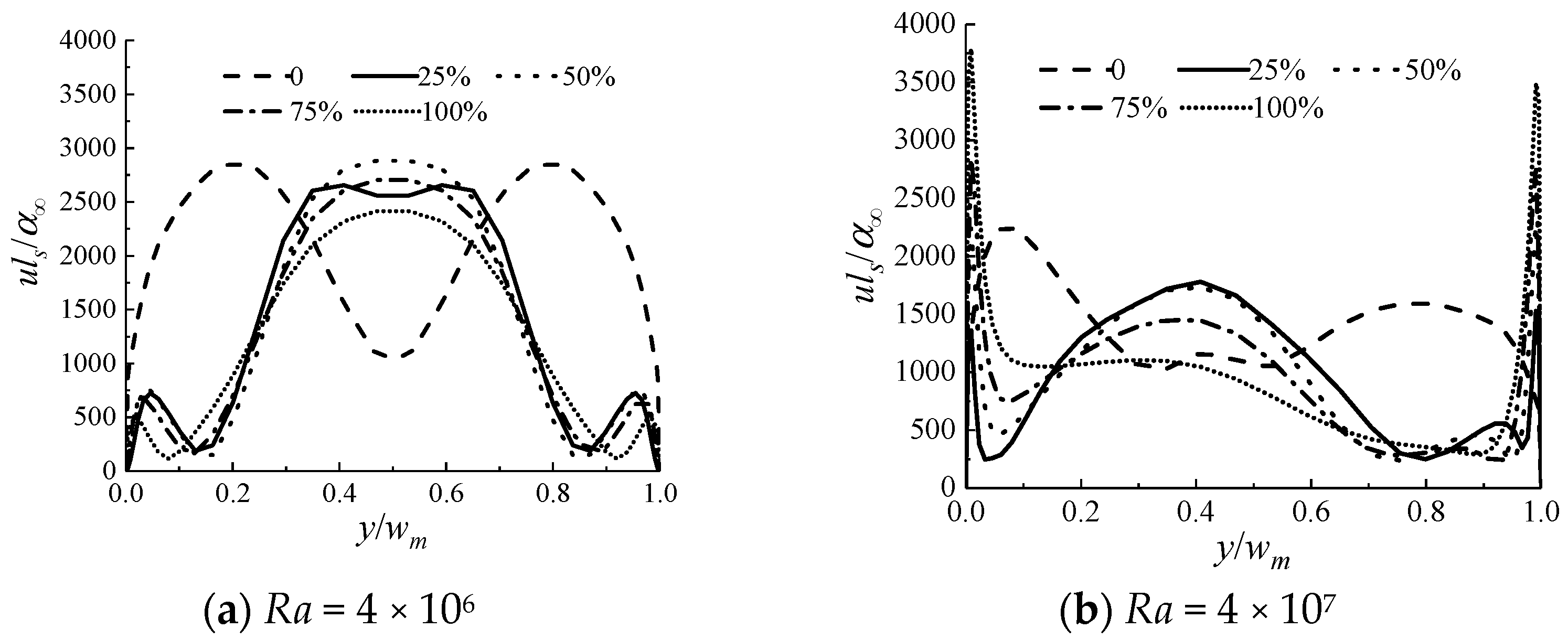
The Rayleigh number significantly affects heat transfer and flow. For high Rayleigh numbers, the steady flows become disturbed and disorderly in the middle corridor. The peak velocity near the heated walls is substantially enhanced for a higher Rayleigh number. As the Rayleigh number increases, the peak sharpens and shifts towards the heated wall, signifying a rapid acceleration of the air in proximity to the heated wall.

(4)

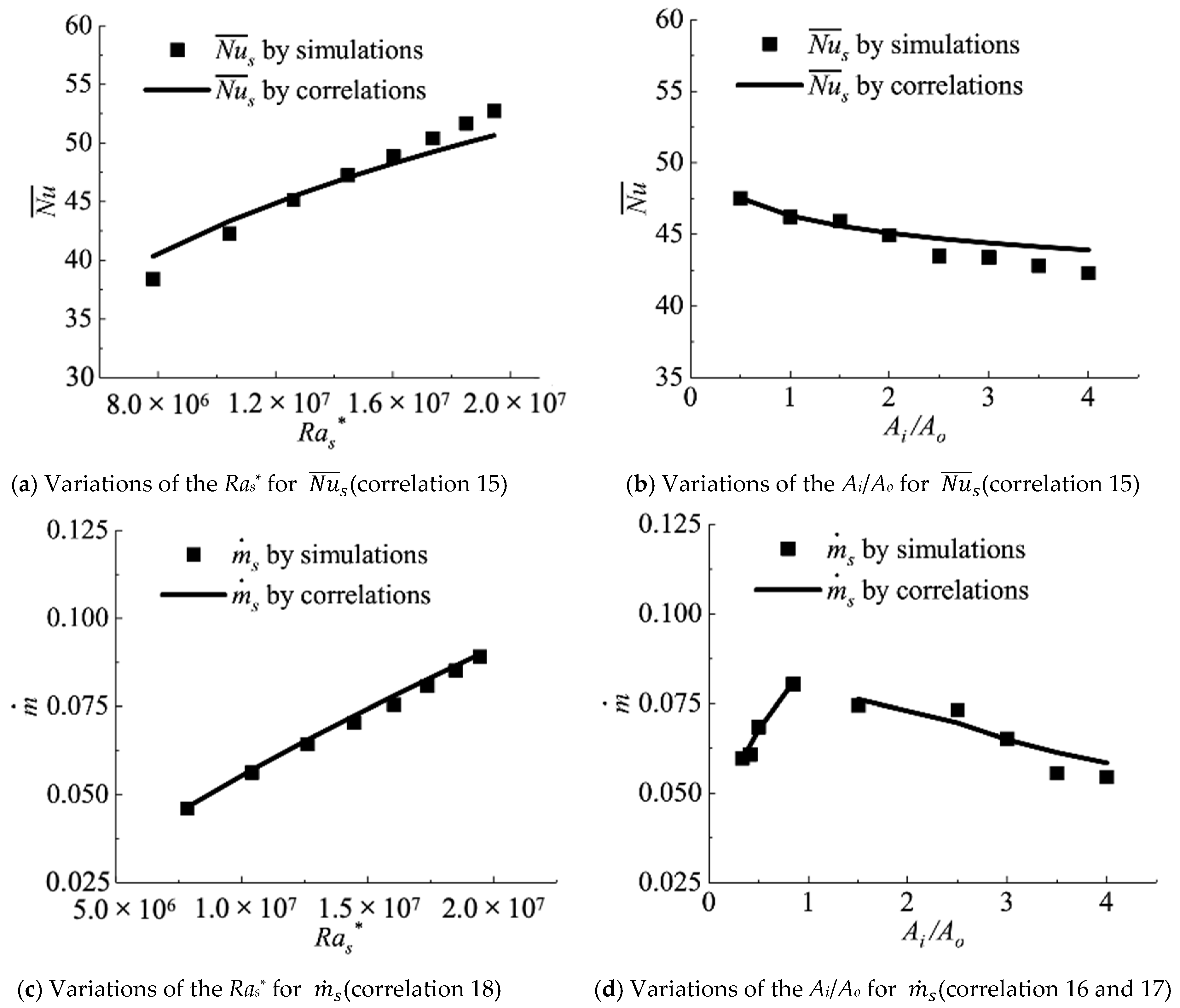
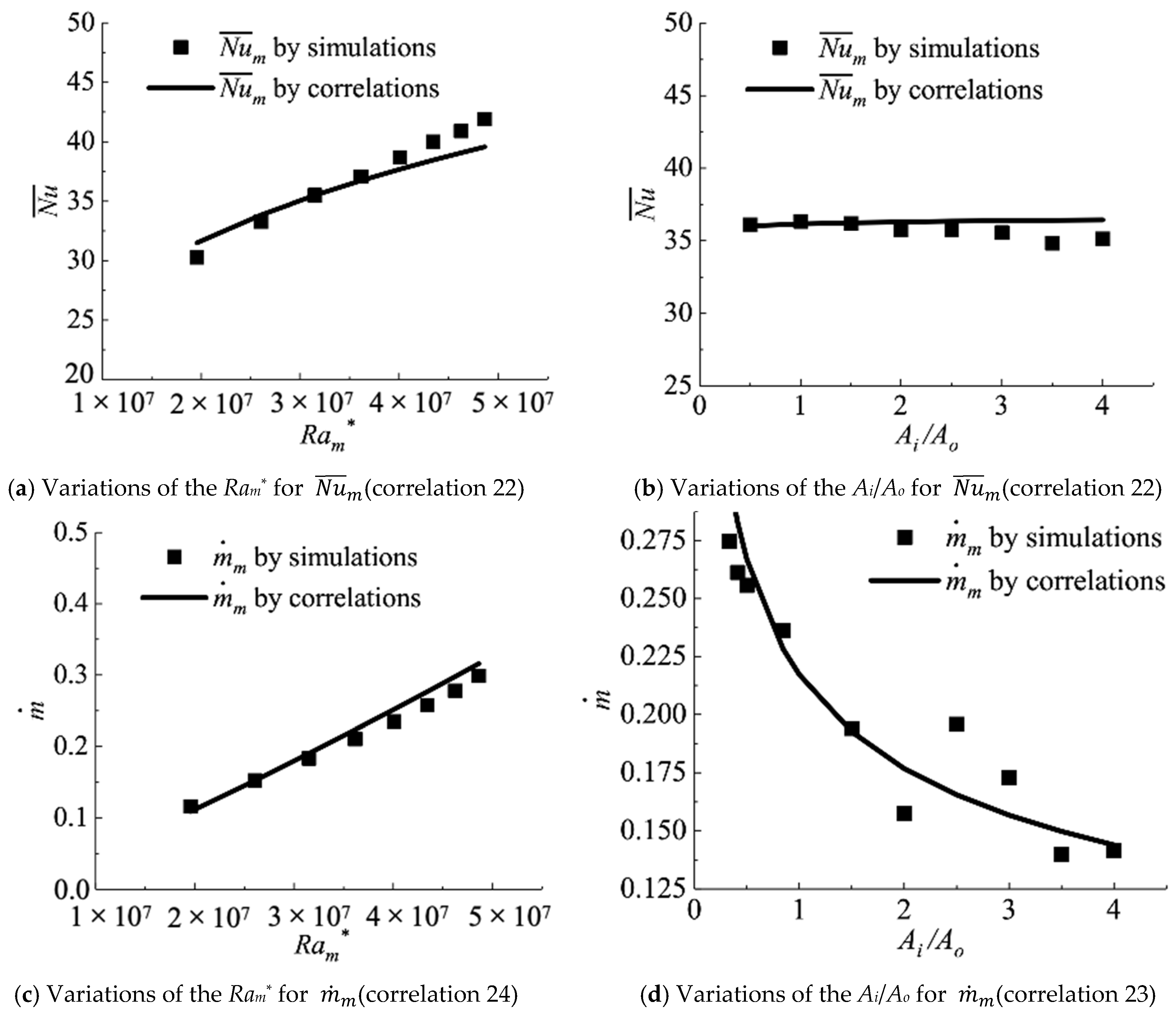
Through theoretical analysis and the fitting of simulation results, semi-empirical correlations have been established to describe the surface-averaged $\overline{Nu}$ of the heated wall as a function of the inlet-to-outlet area ratio and modified Rayleigh number and the induced mass flow rate, ${\dot{m}}_s$, of the channel as a function of the inlet-to-outlet area ratio, modified Rayleigh number, and Prandtl number. These correlations displayed favorable consistency with simulation results, with maximum relative errors of less than 16%.

Notwithstanding, our work is still incomplete and requires further refinement. Future studies will focus on addressing the following: (1) The geometry of the building may influence convective heat exchange within the corridor. Therefore, further investigations need to consider the building’s size, such as its width-to-height ratio or length-to-width ratio. (2) Parameter analysis using a reduced-scale model may yield different results compared to a full-scale building. Future work will entail conducting a study at a full-scale to achieve a better thermal environment within the corridor. (3) The correlations of the air temperature and velocity of the working zone for symmetric or asymmetry heating plants have not been developed. Further studies should investigate these correlations on the convective heat transfer and flow of the channel.

References

1. Wang, H.; Wang, T.; Liu, L.; Long, Z.; Zhang, P. Numerical evaluation of the performances of the ventilation system in a blast furnace casthouse. Environ. Sci. Pollut. Res. 2021, 28, 50668–50682. [Google Scholar] [CrossRef] [PubMed]
2. Liu, F.; Qian, H.; Ma, J.; He, P. A simple model for predicting dispersion characteristics of high-temperature airflow and particle distribution during smelting process in a thermally stratified foundry shop. Energy Build. 2023, 278, 112614. [Google Scholar] [CrossRef]
3. Wang, Y.; Gao, J.; Xing, X.; Liu, Y.; Meng, X. Measurement and evaluation of indoor thermal environment in a naturally ventilated industrial building with high temperature heat sources. Build. Environ. 2016, 96, 35–45. [Google Scholar] [CrossRef]
4. Yi, W.; Chan, A.P. Effects of heat stress on construction labor productivity in Hong Kong: A case study of rebar workers. Int. J. Environ. Res. Public Health 2017, 14, 1055. [Google Scholar] [CrossRef] [PubMed]
5. Wang, Y.; Zhao, T.; Cao, Z.; Zhai, C.; Wu, S.; Zhang, C.; Zhang, Q.; Lv, W. The influence of indoor thermal conditions on ventilation flow and pollutant dispersion in downstream industrial workshop. Build. Environ. 2021, 187, 107400. [Google Scholar] [CrossRef]
6. Rasheed, A.; Lee, J.W.; Kim, H.T.; Lee, H.W. Efficiency of different roof vent designs on natural ventilation of single-span plastic greenhouse. J. Bio-Environ. Control 2019, 28, 225–233. [Google Scholar] [CrossRef]
7. Yang, D.; Dong, S.; Du, T.; Ji, W. Influences of vent location on the removal of gaseous contaminants and indoor thermal environment. J. Build. Eng. 2020, 32, 101679. [Google Scholar] [CrossRef]
8. Aich, W.; Kolsi, L.; Borjini, M.N.; Aissia, H.B.; Öztop, H.; Abu-Hamdeh, N. Three-dimensional CFD Analysis of Buoyancy-driven Natural Ventilation and Entropy Generation in a Prismatic Greenhouse. Therm. Sci. 2016, 52, 1–12. [Google Scholar]
9. Izadyar, N.; Miller, W.; Rismanchi, B.; Garcia-Hansen, V. Impacts of façade openings’ geometry on natural ventilation and occupants’ perception: A review. Build. Environ. 2020, 170, 106613. [Google Scholar] [CrossRef]
10. Bovo, M.; Santolini, E.; Barbaresi, A.; Tassinari, P.; Torreggiani, D. Assessment of geometrical and seasonal effects on the natural ventilation of a pig barn using CFD simulations. Comput. Electron. Agric. 2022, 193, 106652. [Google Scholar] [CrossRef]
11. Yıldız, Ç.; Yıldız, A.E.; Arıcı, M.; Azmi, N.A.; Shahsavar, A. Influence of dome shape on flow structure, natural convection and entropy generation in enclosures at different inclinations: A comparative study. Int. J. Mech. Sci. 2021, 197, 106321. [Google Scholar] [CrossRef]
12. Chati, D.; Bouabdallah, S.; Ghernaout, B.; Tunçbilek, E.; Arıcı, M.; Driss, Z. Turbulent mixed convective heat transfer in a ventilated enclosure with a cylindrical/cubical heat source: A 3D analysis. Energy Sources Part A Recovery Util. Environ. Eff. 2023, 45, 12423–12440. [Google Scholar] [CrossRef]
13. Zhang, W.; Zhao, Y.; Xue, P.; Mizutani, K. Review and development of the contribution ratio of indoor climate (CRI). Energy Built Environ. 2022, 3, 412–423. [Google Scholar] [CrossRef]
14. Tian, G.; Fan, Y.; Wang, H.; Peng, K.; Zhang, X.; Zheng, H. Studies on the thermal environment and natural ventilation in the industrial building spaces enclosed by fabric membranes: A case study. J. Build. Eng. 2020, 32, 101651. [Google Scholar] [CrossRef]
15. Yang, C.; Gao, T.; Li, A.; Gao, X. Buoyancy-driven ventilation of an enclosure containing a convective area heat source. Int. J. Therm. Sci. 2021, 159, 106551. [Google Scholar] [CrossRef]
16. Liu, Q.; Linden, P. The fluid dynamics of an underfloor air distribution system. J. Fluid Mech. 2006, 554, 323–341. [Google Scholar] [CrossRef]
17. Yang, C.; Luo, W.; Li, A.; Gao, X.; Che, L.; Qiao, L.; Gao, T.; Liu, Y. Natural ventilation driven by a restricted heat source elevated to different levels. In Building Simulation; Springer: Berlin/Heidelberg, Germany, 2022; Volume 15, pp. 281–289. [Google Scholar]
18. Tlili, O.; Mhiri, H.; Bournot, P. Empirical correlation derived by CFD simulation on heat source location and ventilation flow rate in a fire room. Energy Build. 2016, 122, 80–88. [Google Scholar] [CrossRef]
19. Park, H.-J.; Holland, D. The effect of location of a convective heat source on displacement ventilation: CFD study. Build. Environ. 2001, 36, 883–889. [Google Scholar] [CrossRef]
20. Su, Y.; Miao, C. The effect of fresh air opening locations on natural ventilation and thermal environment in industrial workshop with heat source. In Proceedings of the 8th International Symposium on Heating, Ventilation and Air Conditioning: Volume 3: Building Simulation and Information Management; Springer: Berlin/Heidelberg, Germany, 2014; pp. 93–100. [Google Scholar]
21. Pu, J.; Yuan, Y.; Jiang, F.; Zheng, K.; Zhao, K. Buoyancy-driven natural ventilation characteristics of thermal corridors in industrial buildings. J. Build. Eng. 2022, 50, 104107. [Google Scholar] [CrossRef]
22. Elenbaas, W. Heat dissipation of parallel plates by free convection. Physica 1942, 9, 1–28. [Google Scholar] [CrossRef]
23. Kihm, K.; Kim, J.; Fletcher, L. Onset of flow reversal and penetration length of natural convective flow between isothermal vertical walls. Trans.-Am. Soc. Mech. Eng. J. Heat Transf. 1995, 117, 776. [Google Scholar] [CrossRef]
24. Habib, M.; Said, S.; Ahmed, S.; Asghar, A. Velocity characteristics of turbulent natural convection in symmetrically and asymmetrically heated vertical channels. Exp. Therm. Fluid Sci. 2002, 26, 77–87. [Google Scholar] [CrossRef]
25. Badr, H.; Habib, M.; Anwar, S.; Ben-Mansour, R.; Said, S. Turbulent natural convection in vertical parallel-plate channels. Heat Mass Transf. 2006, 43, 73–84. [Google Scholar] [CrossRef]
26. Lewandowski, W.M.; Ryms, M.; Denda, H. Natural convection in symmetrically heated vertical channels. Int. J. Therm. Sci. 2018, 134, 530–540. [Google Scholar] [CrossRef]
27. Aung, W.; Worku, G. Developing flow and flow reversal in a vertical channel with asymmetric wall temperatures. J. Heat Transfer. 1986, 108, 299–304. [Google Scholar] [CrossRef]
28. Kim, K.M.; Nguyen, D.H.; Shim, G.H.; Jerng, D.-W.; Ahn, H.S. Experimental study of turbulent air natural convection in open-ended vertical parallel plates under asymmetric heating conditions. Int. J. Heat Mass Transf. 2020, 159, 120135. [Google Scholar] [CrossRef]
29. Cherif, Y.; Sassine, E.; Lassue, S.; Zalewski, L. Experimental and numerical natural convection in an asymmetrically heated double vertical facade. Int. J. Therm. Sci. 2020, 152, 106288. [Google Scholar] [CrossRef]
30. Fedorov, A.G.; Viskanta, R. Turbulent natural convection heat transfer in an asymmetrically heated, vertical parallel-plate channel. Int. J. Heat Mass Transf. 1997, 40, 3849–3860. [Google Scholar] [CrossRef]
31. Yilmaz, T.; Fraser, S.M. Turbulent natural convection in a vertical parallel-plate channel with asymmetric heating. Int. J. Heat Mass Transf. 2007, 50, 2612–2623. [Google Scholar] [CrossRef]
32. Walker, C.; Tan, G.; Glicksman, L. Reduced-scale building model and numerical investigations to buoyancy-driven natural ventilation. Energy Build. 2011, 43, 2404–2413. [Google Scholar] [CrossRef]
33. Wang, M.; Wang, Y.; Liu, L.; Geng, M.; Wang, X.; Qiu, L. Experimental and numerical research of backfill cooling based on similarity theory. J. Build. Eng. 2023, 70, 106380. [Google Scholar] [CrossRef]
34. Pucciarelli, A.; Ambrosini, W. A successful general fluid-to-fluid similarity theory for heat transfer at supercritical pressure. Int. J. Heat Mass Transf. 2020, 159, 120152. [Google Scholar] [CrossRef]
35. Lu, Y.; Dong, J.; Wang, Z.; Wang, Y.; Wu, Q.; Wang, L.; Liu, J. Evaluation of stack ventilation in a large space using zonal simulation and a reduced-scale model experiment with particle image velocimetry. J. Build. Eng. 2021, 34, 101958. [Google Scholar] [CrossRef]
36. Ding, W.; Hasemi, Y.; Yamada, T. Natural ventilation performance of a double-skin façade with a solar chimney. Energy Build. 2005, 37, 411–418. [Google Scholar] [CrossRef]
37. Moosavi, L.; Zandi, M.; Bidi, M.; Behroozizade, E.; Kazemi, I. New design for solar chimney with integrated windcatcher for space cooling and ventilation. Build. Environ. 2020, 181, 106785. [Google Scholar] [CrossRef]
38. Liu, P.-C.; Lin, H.-T.; Chou, J.-H. Evaluation of buoyancy-driven ventilation in atrium buildings using computational fluid dynamics and reduced-scale air model. Build. Environ. 2009, 44, 1970–1979. [Google Scholar] [CrossRef]
39. Etheridge, D.W.; Sandberg, M. Building Ventilation: Theory and Measurement; John Wiley & Sons: Chichester, UK, 1996. [Google Scholar]
40. Walker, C.E. Methodology for the Evaluation of Natural Ventilation in Buildings Using a Reducedscale Air Model. Ph.D. Thesis, Massachusetts Institute of Technology, Cambridge, MA, USA, 2005. [Google Scholar]
41. Shinji, S. Modeling Criteria for the Room Air Motion, Part 1-Practical Similarity Criteria for the Room Air Motion. Pap. Soc. Heat. Air-Cond. Sanit. Eng. Jpn. 1981, 17, 1–10. [Google Scholar]
42. Izadyar, N.; Miller, W.; Rismanchi, B.; Garcia-Hansen, V. A numerical investigation of balcony geometry impact on single-sided natural ventilation and thermal comfort. Build. Environ. 2020, 177, 106847. [Google Scholar] [CrossRef]
43. Farea, T.G.; Ossen, D.R.; Alkaff, S.; Kotani, H. CFD modeling for natural ventilation in a lightwell connected to outdoor through horizontal voids. Energy Build. 2015, 86, 502–513. [Google Scholar] [CrossRef]
44. Liu, J.; Srebric, J.; Yu, N. Numerical simulation of convective heat transfer coefficients at the external surfaces of building arrays immersed in a turbulent boundary layer. Int. J. Heat Mass Transf. 2013, 61, 209–225. [Google Scholar] [CrossRef]
45. Wang, Y.; Cao, L.; Huang, Y.; Cao, Y. Lateral ventilation performance for removal of pulsating buoyant jet under the influence of high-temperature plume. Indoor Built Environ. 2020, 29, 543–557. [Google Scholar] [CrossRef]
46. Zhou, Y.; Wang, M.; Wang, M.; Wang, Y. Predictive accuracy of Boussinesq approximation in opposed mixed convection with a high-temperature heat source inside a building. Build. Environ. 2018, 144, 349–356. [Google Scholar] [CrossRef]
47. Menchaca-Brandan, M.A.; Espinosa, F.A.D.; Glicksman, L.R. The influence of radiation heat transfer on the prediction of air flows in rooms under natural ventilation. Energy Build. 2017, 138, 530–538. [Google Scholar] [CrossRef]
48. Serageldin, A.A.; Ye, M.; Radwan, A.; Sato, H.; Nagano, K. Numerical investigation of the thermal performance of a radiant ceiling cooling panel with segmented concave surfaces. J. Build. Eng. 2021, 42, 102450. [Google Scholar] [CrossRef]
49. Jiang, F.; Yuan, Y.; Li, Z.; Zhao, Q.; Zhao, K. Correlations for the forced convective heat transfer at a windward building façade with exterior louver blinds. Sol. Energy 2020, 209, 709–723. [Google Scholar] [CrossRef]
50. Sevilgen, G.; Kilic, M. Numerical analysis of air flow, heat transfer, moisture transport and thermal comfort in a room heated by two-panel radiators. Energy Build. 2011, 43, 137–146. [Google Scholar] [CrossRef]
51. Zhang, Y.-P.; He, Y.-L.; Liu, Y.-H.; Ma, Y.-X.; Li, Y.-R.; Dou, J.-X. Thermal Effects of Building’s External Surfaces in City—Characteristics of Heat Flux into and out of External Wall Surfaces. Chin. Geogr. Sci. 2004, 14, 343–349. [Google Scholar] [CrossRef]
52. Embaye, M.; Al-Dadah, R.; Mahmoud, S. Numerical evaluation of indoor thermal comfort and energy saving by operating the heating panel radiator at different flow strategies. Energy Build. 2016, 121, 298–308. [Google Scholar] [CrossRef]
53. Yigit, C.; Coskun, G.; Buyukkaya, E.; Durmaz, U.; Güven, H.R. CFD modeling of carbon combustion and electrode radiation in an electric arc furnace. Appl. Therm. Eng. 2015, 90, 831–837. [Google Scholar] [CrossRef]
54. Huang, Y.; Tao, Y.; Shi, L.; Liu, Q.; Wang, Y.; Tu, J.; Gan, X. Numerical study of the performance for a curved double-skin façade in summer. Build. Environ. 2023, 233, 110103. [Google Scholar] [CrossRef]
55. El Ghandouri, I.; El Maakoul, A.; Saadeddine, S.; Meziane, M. Design and numerical investigations of natural convection heat transfer of a new rippling fin shape. Appl. Therm. Eng. 2020, 178, 115670. [Google Scholar] [CrossRef]
56. Liu, M.; Jimenez-Bescos, C.; Calautit, J. CFD investigation of a natural ventilation wind tower system with solid tube banks heat recovery for mild-cold climate. J. Build. Eng. 2022, 45, 103570. [Google Scholar] [CrossRef]
57. Acikgoz, O. A novel evaluation regarding the influence of surface emissivity on radiative and total heat transfer coefficients in radiant heating systems by means of theoretical and numerical methods. Energy Build. 2015, 102, 105–116. [Google Scholar] [CrossRef]
58. Falsetti, C.; Kapulla, R.; Paranjape, S.; Paladino, D. Thermal radiation, its effect on thermocouple measurements in the PANDA facility and how to compensate it. Nucl. Eng. Des. 2021, 375, 111077. [Google Scholar] [CrossRef]
59. Zhang, X.; Ge, Y.; Lang, P. Experimental investigation and CFD modelling analysis of finned-tube PCM heat exchanger for space heating. Appl. Therm. Eng. 2024, 244, 122731. [Google Scholar] [CrossRef]
60. Bakkas, M.; Amahmid, A.; Hasnaoui, M. Steady natural convection in a horizontal channel containing heated rectangular blocks periodically mounted on its lower wall. Energy Conv. Manag. 2006, 47, 509–528. [Google Scholar] [CrossRef]
61. Mouhtadi, D.; Amahmid, A.; Hasnaoui, M.; Bennacer, R. Natural convection in a horizontal channel provided with heat generating blocks: Discussion of the isothermal blocks validity. Energy Conv. Manag. 2012, 53, 45–54. [Google Scholar] [CrossRef]
62. Bakkas, M.; Hasnaoui, M.; Amahmid, A. Natural convective flows in a horizontal channel provided with heating isothermal blocks: Effect of the inter blocks spacing. Energy Conv. Manag. 2010, 51, 296–304. [Google Scholar] [CrossRef]
63. Churchill, S.W.; Chu, H.H. Correlating equations for laminar and turbulent free convection from a vertical plate. Int. J. Heat Mass Transf. 1975, 18, 1323–1329. [Google Scholar] [CrossRef]
64. Olsson, C.-O. Prediction of Nusselt number and flow rate of buoyancy driven flow between vertical parallel plates. J. Heat Transf. 2004, 126, 97–104. [Google Scholar] [CrossRef]
65. Song, C.; Nie, B.; Xu, F. Scaling analysis of natural convection in a vertical channel. Int. Commun. Heat Mass Transf. 2020, 117, 104739. [Google Scholar] [CrossRef]
66. Franco, A.T.; Santos, P.R.; Lugarini, A.; Loyola, L.T.; De Lai, F.C.; Junqueira, S.L.; Nardi, V.G.; Ganzarolli, M.M.; Lage, J.L. The effects of discrete conductive blocks on the natural convection in side-heated open cavities. Appl. Therm. Eng. 2023, 219, 119613. [Google Scholar] [CrossRef]
67. Nghana, B.; Tariku, F.; Bitsuamlak, G. Numerical assessment of the impact of transverse roughness ribs on the turbulent natural convection in a BIPV air channel. Build. Environ. 2022, 217, 109093. [Google Scholar] [CrossRef]
Figure 1. Description of thermal corridors.
Buildings 14 01406 g001
Figure 2. Diagram of scaled experimental model.
Buildings 14 01406 g002
Figure 3. Computational domain.
Buildings 14 01406 g003
Figure 4. Computational grid.
Buildings 14 01406 g004aBuildings 14 01406 g004b
Figure 5. Grid-sensitivity test.
Buildings 14 01406 g005
Figure 6. Comparisons of the CFD simulations and experimental results on opening velocity and corridor vertical temperature.
Buildings 14 01406 g006
Figure 7. Distribution of temperature at x = 1/2L of the side corridor. Simulation settings: (a) standard case: Tw = 80 °C, T = 25 °C, Ao = 0.1875 m2, Ai = 0.1875 m2, ls = 0.2 m, ws = 0.1 m; (b) Tw = 60 °C; (c) Tw = 100 °C; (d) T = 28 °C; (e) T = 22 °C; (f) Ao = 0.125 m2; (g) Ai = 0.125 m2; (h) ls = 0.1 m; (i) ls = 0.3 m; (j) ws = 0.05 m; (k) ws = 0.15 m; (l) sketch of the side corridor.
Buildings 14 01406 g007
Figure 8. Distribution of streamlines at x = 1/2L of the side corridor. Simulation settings: (a) standard case: Tw = 80 °C, T = 25 °C, Ao = 0.1875 m2, Ai = 0.1875 m2, ls = 0.2 m, ws = 0.1 m; (b) Tw = 60 °C; (c) Tw = 100 °C; (d) T = 28 °C; (e) T = 22 °C; (f) Ao = 0.125 m2; (g) Ai = 0.125 m2; (h) ls = 0.1 m; (i) ls = 0.3 m; (j) ws = 0.05 m; (k) ws = 0.15 m.
Buildings 14 01406 g008
Figure 9. Reverse flow on the cold wall from a horizontal inlet under asymmetric heating.
Buildings 14 01406 g009
Figure 10. Temperature profiles along the side corridor at x = 1/2L of different sections.
Buildings 14 01406 g010
Figure 11. Velocity profiles along the side corridor at x = 1/2L of different sections.
Buildings 14 01406 g011
Figure 12. Distribution of temperature at x = 1/2L of the middle corridor. (a) standard case: Tw = 80 °C, T = 25 °C, Ao = 0.1875 m2, Ai = 0.1875 m2, ls = 0.2 m, wm = 0.25 m; (b) Tw = 60 °C; (c) Tw = 100 °C; (d) T = 28 °C; (e) T = 22 °C; (f) Ao = 0.125 m2; (g) Ai = 0.125 m2; (h) ls = 0.1 m; (i) ls = 0.3 m; (j) wm = 0.15 m; (k) wm = 0.35 m; (l) sketch of the middle corridor.
Buildings 14 01406 g012
Figure 13. Distribution of streamlines at x = 1/2L of the middle corridor. (a) standard case: Tw = 80 °C, T = 25 °C, Ao = 0.1875 m2, Ai = 0.1875 m2, ls = 0.2 m, wm = 0.25 m; (b) Tw = 60 °C; (c) Tw = 100 °C; (d) T = 28 °C; (e) T = 22 °C; (f) Ao = 0.125 m2; (g) Ai = 0.125 m2; (h) ls = 0.1 m; (i) ls = 0.3 m; (j) wm = 0.15 m; (k) wm = 0.35 m.
Buildings 14 01406 g013
Figure 14. Reverse flow on the heated walls under symmetric heating.
Buildings 14 01406 g014
Figure 15. Temperature profiles along the middle corridor at x = 1/2L of different sections.
Buildings 14 01406 g015
Figure 16. Velocity profiles along the middle corridor at x = 1/2L of different sections.
Buildings 14 01406 g016
Figure 17. Schematic of flow in the side channel.
Buildings 14 01406 g017
Figure 18. Comparison of surface-averaged N u ¯ s of the heated vertical plate and induced flow rate, m ˙ s , of the side channel between simulations and correlations.
Buildings 14 01406 g018
Figure 19. Schematic of flow in the middle channel.
Buildings 14 01406 g019
Figure 20. Comparison of surface-averaged N u ¯ m of the heated vertical plate and induced flow rate, m ˙ m , of the middle channel between simulations and correlations.
Buildings 14 01406 g020