


Statistical Evaluation of Sleeve Friction to Cone Resistance Ratio in Coarse-Grained Soils


Abstract
1. Introduction
2. Theoretical Basis for the Analysis of Soil Behaviour in Line with Data from the CPT
3. Analysis and Evaluation of Statistical Data
- Clayey fine sand (c f S);
- Silty fine sand (sl f S);
- Fine sand (f S);
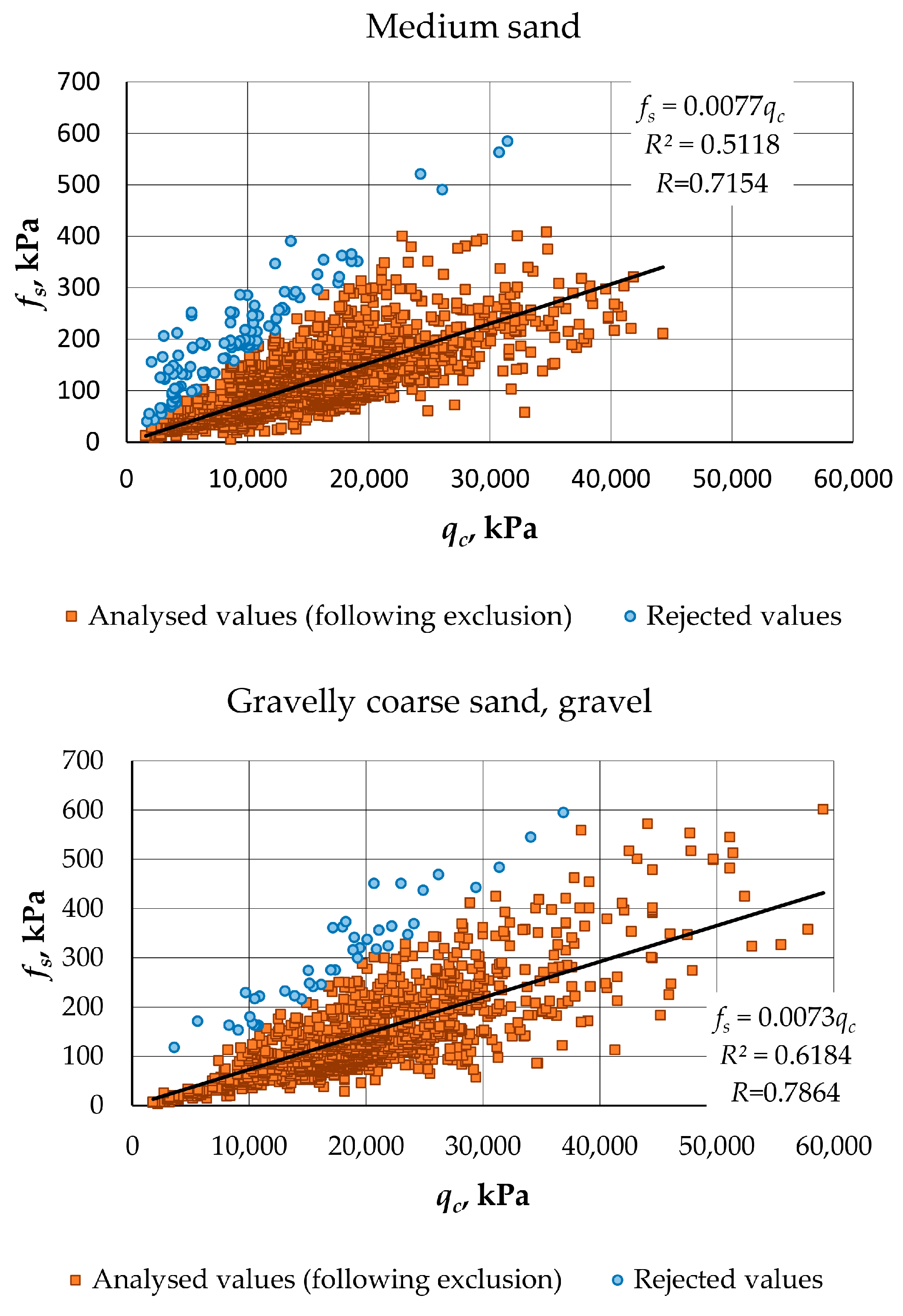
- Medium sand (m S);
- Gravelly coarse sand (g c S);
- Gravel (G).
4. Conclusions and Suggestions
- A statistical analysis of the tested soil showed that the correlational relationship of the tested coarse-grained soil between the sleeve friction and cone resistance in the studied sample (5634 observations) is strong and reaches R = 0.7815. The obtained relationship of the sample is fs = 0.0082qc.
- Regarding the boreholes, six samples of different soils were identified: silty fine sand, clayey fine sand, fine sand, medium sand, gravelly coarse sand and gravel. The difference between the samples of gravelly coarse sand and gravel was found to be statistically insignificant (0.11049). The other samples showed statistically significant differences.
- Statistically different samples like silty fine sand, clayey fine sand, fine sand, medium sand and gravelly coarse sand mixed with gravel were identified. The soils of these isolated groups have a strong correlation between the local sleeve friction and cone resistance (R = 0.7154…0.8510).
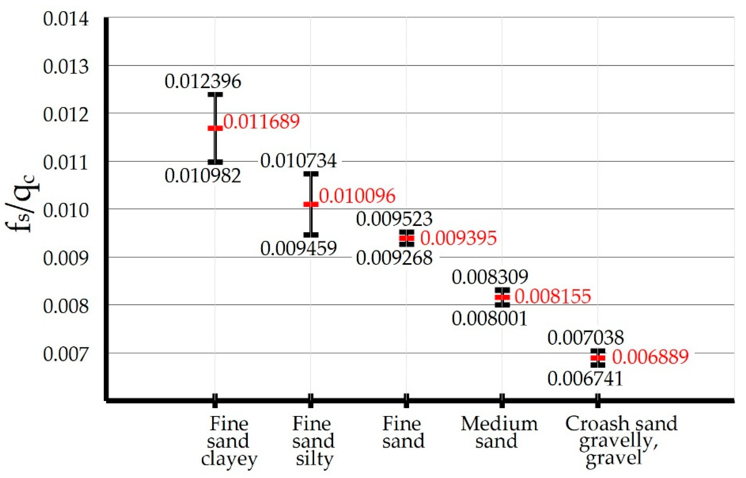
- The statistical analysis of the tested soil showed a confidence level of 95% and determined that the fs/qc ratio is not lower than the ratio calculated for silty fine sand, reaching 0.009459; for clayey fine sand, this ratio is equal to 0.010982, for fine sand, it reaches 0.009268, for medium sand, it is 0.008001 and for gravelly coarse sand and gravel, it is 0.006741. An increase in the particle size of sandy soil leads to a decrease in the ratio between the local sleeve friction and cone resistance.
- The determined fs/qc values are applicable only to the tested types of soil. In order to apply fs/qc ratios to the classification of coarse-grained soils, performing a statistical analysis of CPT data in a specific area is required. The studied relationships between fs and qc in five identified statistically different groups of soil demonstrated a strong relationship between the above-mentioned indicators, thus providing linear equations for the established relationships. The relationships found are valid only for the tested soils. For a broader application, additional research is needed.
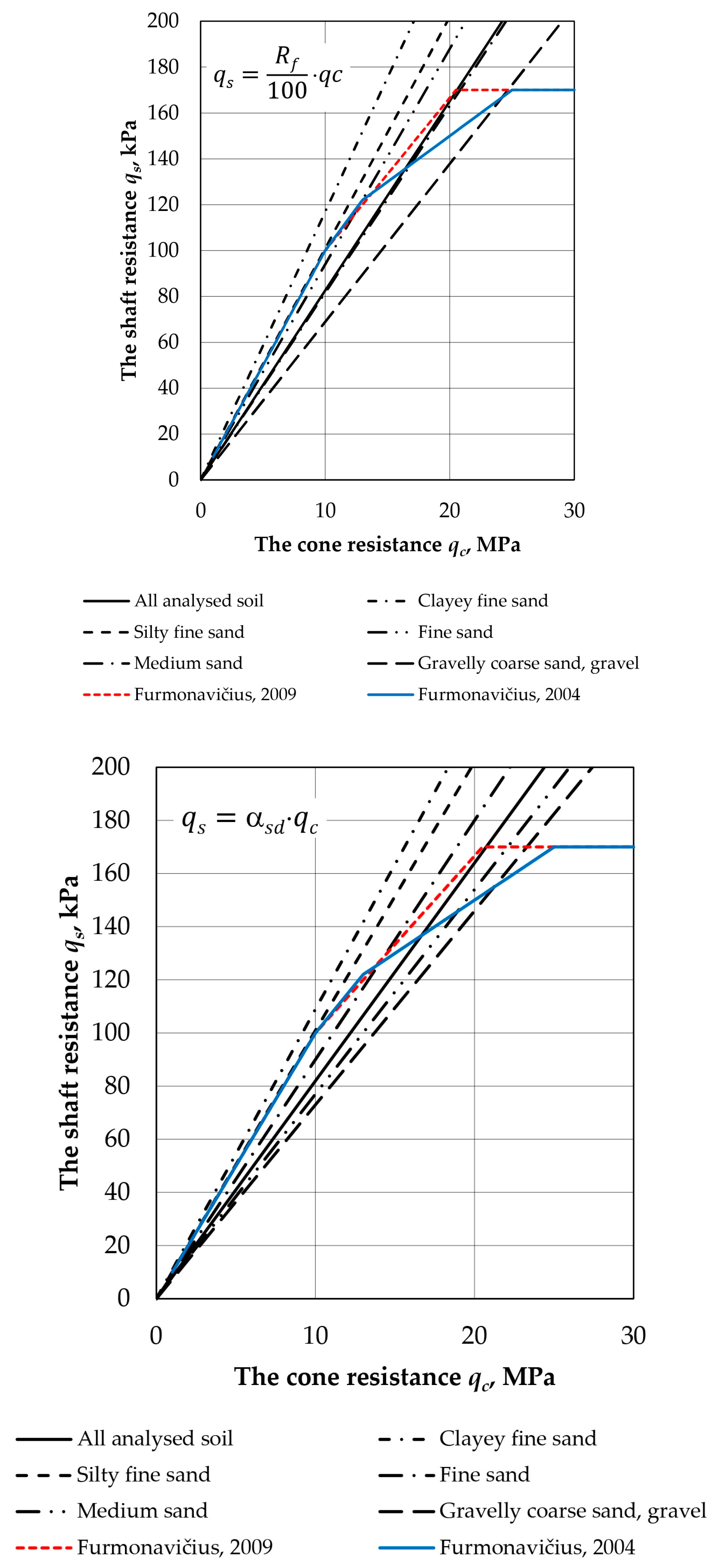
- The study showed that the shaft resistance qs values currently used in pile load-bearing capacity calculations can be more accurately estimated using αsd or Rf/100% for finer coarse-grained soil types, depending on the granulometric composition. However, to determine exact values, more extensive studies are needed, including larger soil samples and evaluating additional properties of the gravel (origin, moisture, etc.).
Author Contributions
Funding
Data Availability Statement
Conflicts of Interest
References
- Yu, X.; Liu, S.; Pei, H. Design of Cone Penetration Test Data Relay Transmission by Magnetic Communication. Sensors 2022, 22, 4777. [Google Scholar] [CrossRef] [PubMed]
- Islam, M.N.; Gnanendran, C.T.; Sivakumar, S.T. Interpretation of Cone Penetration Test Data of an Embankment for Coupled Numerical Modeling. Appl. Mech. 2022, 3, 14–45. [Google Scholar] [CrossRef]
- Guo, Y.; Li, J.; Yu, X. Experimental Study on Load-Carrying Behavior of Large Open-Ended Pipe Pile in Cohesionless Soils. Sustainability 2022, 14, 12223. [Google Scholar] [CrossRef]
- Zwara, Ł.; Bałachowski, L. Prediction of Pile Shaft Capacity in Tension Based on Some Direct CPT Methods—Vistula Marshland Test Site. Materials 2022, 15, 2426. [Google Scholar] [CrossRef] [PubMed]
- Begemann, H.K.S. The friction jacket cone as an aid in determining the soil profile. In Proceedings of the 6th ICSMFE, Montreal, QC, Canada, 8–15 September 1965; Volume 2, pp. 17–20. [Google Scholar]
- Douglas, B.J.; Olsen, R.S. Soil classification using electric cone penetrometer. In Proceedings of the Symposium on Cone Penetration Testing and Experience, Geotechnical Engineering Division, ASCE, St. Louis, MI, USA, October 1981; American Society of Civil Engineers: New York, NY, USA, 1981; pp. 209–227. [Google Scholar]
- Robertson, P.K. In sifu testing and its application to foundation engineering. Can. Geotech. J. 1986, 23, 573–594. [Google Scholar] [CrossRef]
- Robertson, P.K.; Campanella, R.G.; Gillespie, D.; Greig, J. Use of piezometer cone data. In Proceedings of the In-Situ’86 Use of In-Situ Testing in Geotechnical Engineering, ASCE Specialty Conference, Blacksburg, VA, USA, 23–25 June 1986; pp. 1263–1280. [Google Scholar]
- Robertson, P.K. Soil classification using the cone penetration test. Can. Geotech. J. 1990, 27, 151–158. [Google Scholar] [CrossRef]
- Robertson, P.K. Interpretation of cone penetration tests—A unified approach. Can. Geotech. J. 2009, 46, 1337–1355. [Google Scholar] [CrossRef]
- Robertson, P.K. Cone Penetration Test (CPT)-Based Soil Behaviour Type (SBT) Classification System—An Update. Can. Geotech. J. 2016, 53, 1910–1927. [Google Scholar] [CrossRef]
- Vukicevic, M.; Marjanović, M.; Pujevic, V.; Obradović, N. Evaluation of methods for predicting axial capacity of jacked-in and driven piles in cohesive soils. Gradevinar 2018, 70, 685–693. [Google Scholar] [CrossRef]
- Robertson, P.K. Soil behaviour type from the CPT: An update. In Proceedings of the 2nd International Symposium on Cone Penetration Testing, CPT’10, Huntington Beach, CA, USA, 9–11 May 2010. [Google Scholar]
- Cho, S.; Kim, H.-S.; Kim, H. Locally Specified CPT Soil Classification Based on Machine Learning Techniques. Sustainability 2023, 15, 2914. [Google Scholar] [CrossRef]
- New Arc. Handbook for the Building Designer and Builder; New Arc: Kaunas, Lithuania, 2009; 1520p. (In Lithuanian) [Google Scholar]
- Technika. Civil Engineer Handbook; Technika: Vilnius, Lithuania, 2004; 1096p. (In Lithuanian) [Google Scholar]
- EN 1997–1: 2004; Eurocode 7–Geotechnical Design, Part 1: General Rules. The European Union: Maastricht, The Netherlands, 2004.
- Pabedinskaitė, A.; Činčikaitė, R. Quantitative Modeling Methods; Vilnius Gediminas Technical University Publishing House: Vilnius, Lithuania, 2016; (In Lithuanian). [Google Scholar] [CrossRef]


| ξ for n= | 1 | 2 | 3 | 4 | 5 | 7 | 10 |
|---|---|---|---|---|---|---|---|
| ξ3 | 1.40 | 1.35 | 1.33 | 1.31 | 1.29 | 1.27 | 1.25 |
| ξ4 | 1.40 | 1.27 | 1.23 | 1.20 | 1.15 | 1.12 | 1.08 |
| Type of Pile | γR;s | γR;b |
|---|---|---|
| Driven | 1.10 | 1.10 |
| Bored displacement | 1.10 | 1.35 |
| Continuous flight auger (CFA), bored | 2.00 | 1.50 |
| Soil Type | qc, MPa | αs, kPa | αb, MPa | qs;max, kPa | qb;max, MPa |
|---|---|---|---|---|---|
| Clay (moraine) | <5 | 0.050 | 1.0 * | 200 | 6.5 |
| ≥5 | 0.8 * | ||||
| Clay | 0.035 | 1.0 | 150 | ||
| Silt | 0.025 | 0.6 | 150 | ||
| Sand [16] | ≤10 | 0.010 * | 0.5 | 170 | |
| ≥25 | 0.008 * | ||||
| Sand [15] | ≤10 | 0.010 | |||
| >10 | qs = 110 + 4·(qc − 10) |
| Interpretation | Correlation Coefficient R |
|---|---|
| Weak correlational relationship or no correlation | 0 … ±0.3 |
| Moderate correlational relationship | 0.3 … 0.7 −0.3 … −0.7 |
| Strong correlational relationship | 0.7 … 0.9 −0.7 … −0.9 |
| Very strong correlational relationship | 0.9 … 1.0 −0.9 … −1.0 |
| All (Following Exclusion) | All (Prior to Exclusion) | |
|---|---|---|
| Mean | 0.008606 | 0.009320 |
| Standard Error | 4.41 × 10⁻⁵ | 6.48 × 10⁻⁵ |
| Median | 0.008257 | 0.008479 |
| Standard Deviation | 0.00332 | 0.00499 |
| Sample Variance | 1.11 × 10⁻⁵ | 2.49 × 10⁻⁵ |
| Kurtosis | −0.233 | 20.518 |
| Skewness | 0.526 | 3.045 |
| Range | 0.017990 | 0.073704 |
| Minimum | 0.000581 | 0.000581 |
| Maximum | 0.018571 | 0.074286 |
| Count | 5678 | 5934 |
| Confidence Level (95.0%) | 8.6625 × 10⁻⁵ | 1.2698 × 10⁻⁴ |
| Clayey Fine Sand | Silty Fine Sand | Fine Sand | Medium Sand | Gravelly Coarse Sand | Gravel | |
|---|---|---|---|---|---|---|
| Mean | 0.011689 | 0.010096 | 0.009395 | 0.008155 | 0.006940 | 0.006699 |
| Standard Error | 3.57 × 10⁻⁴ | 3.22 × 10⁻⁴ | 6.51 × 10⁻⁵ | 7.85 × 10⁻⁵ | 9.61 × 10⁻⁵ | 1.16 × 10⁻⁴ |
| Median | 0.011897 | 0.009661 | 0.009379 | 0.007697 | 0.006174 | 0.006342 |
| Standard Deviation | 4.09 × 10⁻³ | 4.15 × 10⁻³ | 3.29 × 10⁻³ | 3.13 × 10⁻³ | 2.66 × 10⁻³ | 2.29 × 10⁻³ |
| Sample Variance | 1.67 × 10⁻⁵ | 1.72 × 10⁻⁵ | 1.08 × 10⁻⁵ | 9.82 × 10⁻⁶ | 7.07 × 10⁻⁶ | 5.25 × 10⁻⁶ |
| Kurtosis | −0.825 | 0.685 | −0.106 | −0.099 | −0.115 | −0.295 |
| Skewness | 0.248 | 0.927 | 0.341 | 0.663 | 0.730 | 0.556 |
| Range | 0.019161 | 0.021171 | 0.018405 | 0.016965 | 0.013201 | 0.010998 |
| Minimum | 0.004153 | 0.001446 | 0.000811 | 0.000581 | 0.001593 | 0.001973 |
| Maximum | 0.023314 | 0.022617 | 0.019216 | 0.017546 | 0.014795 | 0.012971 |
| Count | 131 | 165 | 2550 | 1593 | 765 | 388 |
| Confidence Level (95.0%) | 0.000707 | 0.000637 | 0.000128 | 0.000154 | 0.000189 | 0.000229 |
| Clayey Fine Sand | Silty Fine Sand | Fine Sand | Medium Sand | Gravelly Coarse Sand | Gravel | |
|---|---|---|---|---|---|---|
| Clayey fine sand | 1.00 × 100 | 1.06 × 10⁻³ | 3.42 × 10⁻⁹ | 1069 × 10−17 | 7.00 × 10⁻²⁶ | 1.59 × 10⁻²⁷ |
| Silty fine sand | 1.00 × 100 | 3.46 × 10⁻² | 2.27 × 10⁻⁸ | 1.86 × 10⁻¹⁷ | 3.46 × 10⁻¹⁹ | |
| Fine sand | 1.00 × 100 | 2.50 × 10⁻³³ | 2.68 × 10−87 | 4.23 × 10−71 | ||
| Medium sand | 1.00 × 100 | 4.43 × 10⁻²² | 1.02 × 10⁻²³ | |||
| Gravelly coarse sand | 1.00 × 100 | 1.11 × 10⁻¹ | ||||
| Gravel | 1.00 × 100 |
| Clayey Fine Sand | Silty Fine Sand | Fine Sand | Medium Sand | Gravelly Coarse Sand + Gravel | |
|---|---|---|---|---|---|
| Mean | 0.011689 | 0.010096 | 0.009395 | 0.008155 | 0.006889 |
| Standard Error | 3.57 × 10⁻⁴ | 3.22 × 10⁻⁴ | 6.51 × 10⁻⁵ | 7.85 × 10⁻⁵ | 7.58 × 10⁻⁵ |
| Median | 0.011897 | 0.009661 | 0.009379 | 0.007697 | 0.006290 |
| Standard Deviation | 4.09 × 10⁻³ | 4.15 × 10⁻³ | 3.29 × 10⁻³ | 3.13 × 10⁻³ | 2.58 × 10⁻³ |
| Sample Variance | 1.67 × 10⁻⁵ | 1.72 × 10⁻⁵ | 1.08 × 10⁻⁵ | 9.82 × 10⁻⁶ | 6.65 × 10⁻⁶ |
| Kurtosis | −0.825 | 0.685 | −0.106 | −0.099 | −0.041 |
| Skewness | 0.248 | 0.927 | 0.341 | 0.663 | 0.727 |
| Range | 0.019161 | 0.021171 | 0.018405 | 0.016965 | 0.013026 |
| Minimum | 0.004153 | 0.001446 | 0.000811 | 0.000581 | 0.001593 |
| Maximum | 0.023314 | 0.022617 | 0.019216 | 0.017546 | 0.014519 |
| Count | 131 | 165 | 2550 | 1593 | 1158 |
| Confidence Level (95.0%) | 0.000707 | 0.000637 | 0.000128 | 0.000154 | 0.000149 |
| Clayey Fine Sand | Silty Fine Sand | Fine Sand | Medium Sand | Gravelly Coarse Sand + Gravel | |
|---|---|---|---|---|---|
| Clayey fine sand | 1.00 × 100 | 1.06 × 10⁻³ | 3.42 × 10⁻⁹ | 2.69 × 10⁻¹⁷ | 2.64 × 10⁻²⁶ |
| Silty fine sand | 1.00 × 100 | 3.46 × 10⁻² | 2.27 × 10⁻⁸ | 3.93 × 10⁻¹⁸ | |
| Fine sand | 1.00 × 100 | 2.50 × 10⁻³³ | 1.96 × 10−125 | ||
| Medium sand | 1.00 × 100 | 2.06 × 10⁻³⁰ | |||
| Gravelly coarse sand + gravel | 1.00 × 100 |
| Clayey Fine Sand (c f S) | Silty Fine Sand (st f S) | Fine Sand (f S) | Medium Sand (m S) | Gravelly Coarse Sand, Gravel (c g S + G) | All (Following Exclusion) | |
|---|---|---|---|---|---|---|
| Parameters for linear equations | ||||||
| αsd | 0.0109 | 0.0101 | 0.0090 | 0.0077 | 0.0073 | 0.0082 |
| R2 | 0.6928 | 0.5605 | 0.7242 | 0.5118 | 0.6184 | 0.6108 |
| R | 0.8323 | 0.7487 | 0.8510 | 0.7154 | 0.7863 | 0.7815 |
| Mean values of Rf/100% = fs/qc with a confidence level of 95% | ||||||
| fs/qc | 0.011689 | 0.010096 | 0.009395 | 0.008155 | 0.006889 | 0.008258 |
| Mean values of fs/qc with a confidence level of 95% | ||||||
| from | 0.010982 | 0.009459 | 0.009268 | 0.008001 | 0.006741 | 0.007740 |
| to | 0.012396 | 0.010734 | 0.009523 | 0.008309 | 0.007038 | 0.009472 |
Disclaimer/Publisher’s Note: The statements, opinions and data contained in all publications are solely those of the individual author(s) and contributor(s) and not of MDPI and/or the editor(s). MDPI and/or the editor(s) disclaim responsibility for any injury to people or property resulting from any ideas, methods, instructions or products referred to in the content. |
© 2024 by the authors. Licensee MDPI, Basel, Switzerland. This article is an open access article distributed under the terms and conditions of the Creative Commons Attribution (CC BY) license (https://creativecommons.org/licenses/by/4.0/).
Share and Cite
Sližytė, D.; Šalna, R.; Urbonas, K. Statistical Evaluation of Sleeve Friction to Cone Resistance Ratio in Coarse-Grained Soils. Buildings 2024, 14, 745. https://doi.org/10.3390/buildings14030745
Sližytė D, Šalna R, Urbonas K. Statistical Evaluation of Sleeve Friction to Cone Resistance Ratio in Coarse-Grained Soils. Buildings. 2024; 14(3):745. https://doi.org/10.3390/buildings14030745
Chicago/Turabian StyleSližytė, Danutė, Remigijus Šalna, and Kęstutis Urbonas. 2024. "Statistical Evaluation of Sleeve Friction to Cone Resistance Ratio in Coarse-Grained Soils" Buildings 14, no. 3: 745. https://doi.org/10.3390/buildings14030745
APA StyleSližytė, D., Šalna, R., & Urbonas, K. (2024). Statistical Evaluation of Sleeve Friction to Cone Resistance Ratio in Coarse-Grained Soils. Buildings, 14(3), 745. https://doi.org/10.3390/buildings14030745