Abstract
This study proposes a seismic performance evaluation method for structures using the base shear index to calculate the collapse probability. After non-proportional damping was applied to the three-dimensional bar system model, the structural dynamic response was computed through large-scale finite element analysis. A three-dimensional matrix element for calculating viscous dampers was established in this study. The viscous unified elastoplastic (VUEL) damper element program was compiled using the Fortran language into the ABAQUS 6.14 software. An incremental dynamic analysis (IDA) routine was developed using Python 3.0 within the environment of ABAQUS. The uncontrolled structure was designed using the forced decoupling response spectrum method (FD-RSM), while the damped structure was designed using the complex modal response spectrum method (CM-RSM). Seismic fragility analysis was conducted on both uncontrolled and damped structures using the recommended far-field and near-field earthquake records from ATC-63 FEMAP-695. The shear-based fragility index and collapse probability were investigated to comprehensively assess the seismic performance of the uncontrolled and damped structures. The analysis results indicated that the ratios of the limit performance states for moderate damage (IO), severe damage (LS), and complete damage (CP) in the structure were 1:1.6:2.6. Compared with the various limit performance states of the uncontrolled structures, the increments in the moderate, severe, and complete damage limit performance states of the damped structures were 12.79%, 14.86%, and 16.97%, respectively.
1. Introduction
With advances in engineering technology, the seismic design of high-rise buildings and structures has become a critical issue for ensuring structural safety and enhancing seismic performance. A fragility analysis is an important method for assessing the potential damage and fragility of structures subjected to seismic actions. Seismic fragility analysis primarily predicts the probability of structures reaching or exceeding various damage levels under different types of ground motion excitations, such as different impact velocities, structural frequencies, near-fault and far-field earthquakes [1], and dynamic and static loads [2,3,4]. A fragility curve is regarded as a graphical representation of seismic hazard [5,6]. Fragility can be used to predict the probability of damage to a population of structures under earthquake-induced ground motions. In recent years, as a statistical method to evaluate the structural damage caused by various natural disasters, seismic vulnerability analysis and parameter estimation analysis have been carried out using drift index and strain index, respectively. The research on vulnerability has attracted more and more attention from scholars at home and abroad [7,8,9].
A seismic fragility analysis aims to predict the potential damage and fragility of structures subjected to seismic actions. By conducting incremental dynamic analysis (IDA) to establish fragility curves, which serve as graphical representations of seismic hazards, the cumulative damage and collapse probability of structures under earthquake-induced ground motions can be assessed [10,11]. Fragility curves can provide information on the probability of structural damage at different seismic intensities, thereby offering important references for the seismic design and risk assessment of structures [12]. The group effect of structures can enhance the collapse reserve coefficient [13].
In seismic fragility analysis, factors such as damping and negative stiffness play critical roles. Damping devices have been applied to various structures, including cultural heritage buildings and retrofitted old houses, tunnels, and bridges [14,15,16,17,18,19,20]. Particle system random matrix theory has been utilized to quantify damping models [21,22], and optimal damping and corresponding damping parameters have been identified [23,24,25,26]. The introduction of damping devices into structures can absorb and dissipate seismic energy, reduce the structural response [27], and improve the structural comfort [28], with the hysteresis curve used to reflect the relationship between the characteristic parameters of dampers and the main structural response [29,30]. Negative stiffness can change the stiffness characteristics of structures without impairing their functionality [31,32], thus further improving the seismic performance of structures and reducing the non-linear response [33,34]. Therefore, accurately assessing the impact of damping devices and negative stiffness on the seismic performance of structures is of great significance for guiding the seismic design and optimizing the seismic performance of structures.
Over the past few decades, extensive research has been conducted on seismic fragility. However, with the emergence of complex structures and multi-degree-of-freedom systems, traditional modal analysis methods have been unable to accurately assess complex structures. The difference between the real modes in practical modal theory and the complex modes in complex modal theory lies in the magnitude of the phase differences at the peak points. An enhanced truncation method for nonclassical damping systems in a complex modal analysis was proposed. Therefore, the introduction of complex modal analysis methods has become an effective approach for addressing this issue. This provides a theoretical basis for the finite element numerical analysis of non-classical damping structures. Scholars have developed user subroutines for damped bearings [35] and conducted relevant research on extending the finite element method [36,37]. Furthermore, simplified connection elements were used to simulate the dampers, and there were relatively few programs for viscous dampers applied to three-dimensional structures, which limited the seismic performance analysis of the non-proportional damping structure.
The aforementioned scholars conducted relevant research on the theory of non-proportional damping structures and seismic performance. When analyzing the structural seismic performance, they used particle system models or 2D simplified models without considering the spatial characteristics of the structure, the uneven distribution of mass and stiffness, and the coupling effect of the structure when subjected to 3D seismic input. This study proposes an evaluation method for structural seismic performance that utilizes the structural shear fragility index to calculate the collapse probability. After non-proportional damping was applied to the three-dimensional bar system model, the structural dynamic response is computed through large-scale finite element analysis. This study establishes a 3D matrix element for calculating the viscous dampers. The universal viscous damper unit is compiled into the VUEL subroutine of ABAQUS 6.14 software in Fortran programming language. Additionally, a fragility program is developed for ABAQUS software using Python 3.0. This paper applies the developed ABAQUS damper element to a three-dimensional damped structure, deriving shear-based vulnerability indices for various performance points. The seismic record sets recommended by ATC-63 in FEMAP-695, including far-field and near-field earthquake records, are utilized. A numerical comparative analysis between uncontrolled structures and damped structures is conducted using ABAQUS software through incremental dynamic analysis (IDA). Shear-based vulnerability indices of different performance points are proposed to further determine whether the underlying structure has brittle failure so as to comprehensively evaluate the seismic performance of the structure.
2. The Complex Mode Superposition Method for 3D Structures
The present study extended the non-proportional damping approach to the vibration analysis of three-dimensional structures. This study applied the complex mode superposition response spectrum method to conduct the spectral analysis and design of the non-proportionally damped structures and then carried out the vulnerability analysis of the structures. The aim was to describe the dynamic response and energy dissipation characteristics of structures during the vibration process more accurately. This provided a more precise and reliable method of vibration analysis in the field of structural engineering.
For a structure equipped with viscous dampers (viscous dampers and supports), the motion equations of the structure can be written as follows [38]:
where , , and are the mass, damping, and stiffness matrices of the structure without the damper, respectively. represents the external load.
where and represent the mass and rotational inertia of the -th layer, respectively. The rotational inertia is obtained by combining the rotational inertia of the floor and the vertical lateral force-resisting element. Generally, the rotational inertia of the vertical, lateral force-resisting element is much smaller than that of the floor and can be ignored.
where and represent the equivalent length and width of the -th floor slab. For unidirectional earthquake excitation, and ( represents the seismic acceleration vector). For triaxial earthquake excitation, , where and represent the translational displacement in the and directions, respectively, and represents the rotational displacement of the structure.
where , , and represent the seismic acceleration in the , , and directions, respectively. represents a position vector, which denotes the position of the structure in space; .
is the matrix representing the restoring forces of the linear damper.
where is the sum of damping of all dampers in the layer:
By substituting Equation (7) into the motion equation of the structure, we obtain the following:
where is the position matrix of the dampers.
where is the angle between the energy dissipation direction of the damping device on the -th layer and the horizontal plane.
In structural dynamic analysis, two common forms of damping are typically utilized: Rayleigh damping and Cauchy damping. Rayleigh damping is commonly employed to describe the damping characteristics of structures within the low-frequency vibration range. Its expression is as follows:
The Raleigh damping coefficient and are calculated based on the circular frequency and damping ratio corresponding to the first two modes of vibration of the non-classical damping structure.
For classical damping structures, the damping ratio for concrete structures is taken as 0.05, and for steel structures, it is taken as 0.02. The Raleigh damping coefficients and are calculated based on the circular frequency and damping ratio corresponding to the first two modes of vibration.
Caughey damping is typically used to describe the damping characteristics of structures in the high-frequency vibration range, especially when the dominant mechanism of damping occurs within the material. The Cauchy damping calculation usually involves consideration of the non-linear behavior of materials and the dynamic response characteristics of the structure. Its expression is as follows:
In general, Rayleigh damping and Cauchy damping are two different damping models, and the choice of which model to use depends on the characteristics of the structure, the frequency range of vibration, and the physical mechanism of damping behavior.
Under earthquake action, the motion equation of a linear viscously damped system with N degrees of freedom in the system is as follows [38]:
where , , and represent the N × N order structural mass, non-classically damped matrix, and stiffness matrix, respectively, and represents a position vector. To decouple the foregoing equation of motion, it must be transformed into a 2N first-order differential equation of motion, as follows:
In Equation (12),
Matrices and are both symmetric non-positive definite matrices. Typically, the eigenvalue, , corresponding to Equation (12), appears as conjugate pairs. The eigenvector, , has the form (where is the ith vibration deformation mode (i.e., shape mode)). The eigenvalue, , of the non-classically damped system can be expressed as (); and and are the ith order natural frequency and mode damping ratio of the structure, respectively. The damped natural frequency corresponding to can be obtained by the following:
where and represent the real and imaginary parts of a complex number, respectively. Using the mode shape,
where the superscript (“”) indicates conjugation.
In solving the total response of the structure according to the principle of complex vibration type superposition, the displacement vector, , can be expanded as follows:
where is the complex vibration type coordinate matrix. N is the number of modes. This matrix is obtained from the following decoupled complex vibration-type equation of motion (Equation (17)):
where is the participation coefficient of the i-th mode shape. To facilitate the solution, it is converted into the standard single-degree-of-freedom expression:
By considering the derivative form of the Duhamel integral, can be represented by and as follows:
By substituting Equation (19) into Equation (16), the following is derived:
where and . The modal responses and can be solved via typical numerical approaches, such as the Newmark-β method. Compared with Equation (16), the coefficient vector (, ) and unknown quantity () in the foregoing equation are all in the form of real numbers, which are convenient to use in actual calculations. Moreover, the form of the foregoing expression is easy to combine with the response spectrum theory such that the maximum seismic action effect on the structure can be obtained.
In engineering vibration analysis, the structural response quantities of interest typically include inter-story displacements and inter-story drifts, as well as shear forces, bending moments, and so on. These response quantities are associated with displacements. Thus, any seismic response quantity , where is the response transformation vector related to the geometric and physical properties of the structure. Utilizing Equation (20), can be further represented as follows:
where and .
Assuming the seismic acceleration time history is a zero-mean Gaussian stationary process, the peak response coefficients of each mode are equal to the total response peak coefficient. Utilizing the method of contour integration, we can derive the expression for the maximum value of as a combination of peak responses for each mode; accordingly, the maximum response of the structure is
where and correspond to and , representing the velocity spectral value and displacement spectral value of the -th order vibration mode, respectively. For convenience, velocity spectra are typically replaced by pseudo-velocity spectra. , , and represent the mode correlation coefficients for velocity–velocity, velocity–displacement, and displacement–displacement, respectively, and they have the following expressions: , , and are the crest factor ratios ( denotes the crest factor of response g, and and represent the shape responses and of the mode, respectively).
Equation (22) denotes the method of complex mode decomposition response spectrum under three-dimensional seismic action.
During the structural grid partitioning, the floor slabs were divided according to a 1.5 m × 1.5 m grid, and the frame beams and columns were divided based on a length of 1.5 m (Figure 1c,d). All degrees of freedom at the base of the structural frame columns were constrained, and a uniform seismic excitation method was used (see Figure 1).
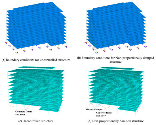
Figure 1.
Three-dimensional finite element models for structures.
3. Viscous Damper Element in ABAQUS
Dampers (Figure 2) were applied to the three-dimensional structure (Figure 1d) while also considering the influence of support connections on the structure. It is necessary to transform the elemental property matrix established in the local coordinate system of the element into the overall coordinate system of the system (Equation (26)). The process of ABAQUS subroutine development is shown in Figure 3. The process of program development using ABAQUS started with defining the initial conditions, followed by initiating the analysis step and the increment step. During the increment step, integral point values were calculated from node values, and the iteration began. The program calculated the strain increment and the stress increment, updated the stress, defined the loads, and solved the system. Finally, the program evaluated the convergence of results. If the evaluation indicated convergence, the process continued accordingly. The transformation matrix from the local to global coordinates is given by the following equation:
where and represent the forces or displacements of the element in the global coordinate system and local coordinate system, respectively. The transformation matrix of dimension (12 × 12) was composed of a matrix of dimension (3 × 3).
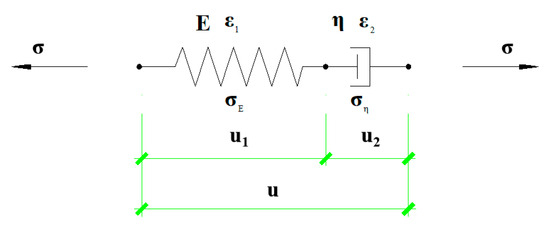
Figure 2.
MAXWELL model.
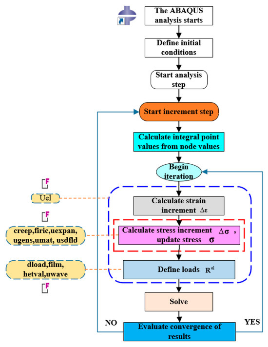
Figure 3.
The process of ABAQUS subroutine development.
In this matrix, is the direction cosine matrix.
where , , and represent the cosines of the angles between the axis and the , , and axes of the coordinate system. Similarly, , , and represent the cosine values of the angles between the axis and the , , and axes, respectively. The , , and axes correspond to the axis. The direction cosines and matrix can be obtained from the coordinates of Points 1, 2, and 3, as follows:
similarly, let us denote as the unit vector along the -axis.
The unit vector along the axis is given by the following equation, where is the distance between Points 1 and 3:
The cross product of two vectors is given by the following determinant:
Finally, we can obtain the direction cosines of the axis.
The forces at the two ends of the node in the global coordinate system [39,40,41] are as follows:
If stiffness is not considered, . When an and are present, indicating a linear segment, Equation (35) can be transformed into a linear segment according to
which results in
The overall stiffness matrix for a linear viscous damping element is
where denotes a specific variable or parameter. is the HHT integration damping constant, which typically ranges from −0.5 to 0. In ABAQUS, the value of is commonly set to −0.05.
The residual vector for each degree of freedom at the node is given by
When , is present and the segment is non-linear, Equation (25) can be transformed into
where
The calculation method for the energy dissipation increment of the damper proposed in reference [42] was used.
The energy dissipation increment of the damper at the time step can be obtained through numerical integration using the trapezoidal rule.
Therefore, the overall stiffness matrix for a non-linear viscous damping unit is defined as
4. Fragility Analysis for Structural Shear
4.1. Seismic Probabilistic Demand Analysis
In the seismic probabilistic demand model, it is assumed that under the seismic intensity , the seismic demand D follows a log-normal distribution [43]. The probabilistic seismic demand model can be written as follows [44]:
where represents the median value of the conditional seismic demand , and denotes the logarithmic standard deviation.
The regression relationship between the median value of the seismic demand and seismic intensity typically follows a power law function.
Taking the logarithm of both sides of Equation (47):
where and . Equation (47) can be linearly fitted with coefficients and based on the results of IDA.
4.2. Structural Seismic Fragility Analytical Function
Seismic fragility is a critical indicator in earthquake risk assessment and is used to assess the seismic resistance and fragility of structures during earthquakes. The seismic fragility function, denoted as , can be obtained by convolving the seismic demand and probabilistic seismic capacity models.
where is the median value of the conditional seismic demand D, and is the logarithmic standard deviation. Substituting into Equation (48):
where
According to the solution based on the average and standard deviation of the probability distribution, the response parameters of the structures (displacement, stress, damage index, etc.) under seismic action follow a log-normal distribution and can be expressed as follows:
The probability density function is
The fragility curve of the structure is represented as follows:
in which
where represents a function that follows a standard normal distribution, and and denote the median value and logarithmic standard deviation required for the structure to achieve a certain performance level, respectively.
4.3. Shear Ratio Coefficients for Different Limit State Performance Points
The shear index for each performance point was derived from the drift index, and the correlation coefficients were obtained using a data fitting method as per the requirements of academic papers. Based on the results of seismic probability demands [44], the following Equation (58) was derived through data fitting:
where represents the shear force at the bottom of the structure, and represents the structural drift index. and represent the IDA curves for the structural shear force, and and are the coefficients obtained from the seismic probability demand curves. In power function relationships, a and b represent the scale and exponent parameters, respectively, and they have different effects on uncontrolled and damped structures. The influence of the scale parameter a is as follows. For uncontrolled structures, the magnitude of the scale parameter a reflects the maximum shear force level that the structure sustains under seismic action. A larger-scale parameter implies that the structure experiences greater forces during earthquakes and can therefore be used to evaluate the seismic performance and safety margin of the structure. In damped structures, scale parameter a reflects the maximum shear force sustained by the structure under seismic action. However, compared with uncontrolled structures, owing to the effect of damping measures, the scale parameter a of the damped structure is relatively reduced, indicating that the seismic forces sustained by the structure under the same seismic action may be lower, thus reducing the risk of structural damage. The influence of the exponent parameter b is as follows. For uncontrolled structures, the exponent parameter b reflects the dynamic characteristics of the structure, including the stiffness and energy dissipation capacity. A smaller b usually indicates that the structure has a greater deformation and energy dissipation capacity, but this may also mean that the structure is more sensitive to seismic actions. In damped structures, the exponent b is influenced by the damping devices. Well-designed damping devices can alter the stiffness and damping characteristics of the structure, thereby affecting the value of the exponent parameter b. Through an appropriate design of damping devices, the exponent parameter b of the damped structure can be adjusted to enhance its seismic performance:
The combination of structural bottom shear forces corresponding to different performance points is calculated as follows:
disregarding vertical seismic motion:
where , , and represent the shear forces in , , and , respectively. The shear ratio coefficients for different limit state performance points were determined.
where denotes the structural shear force calculated using the CCQC superposition method for complex vibrations, which was combined by shear components in three directions.
5. Case Study Analysis
5.1. Structural Design Information
A performance-based seismic design method was employed to analyze a 10-story benchmark reinforced concrete structure (Figure 4a,b). The design reference period for the structure is set at 50 years. The seismic defense level of the structure was classified as B with a design ground motion intensity of 8 (0.20 g), and the site was categorized as Class I. The seismic design belongs to the first group, with a safety level of II and a characteristic period of 0.20 s. The damping ratio of the ordinary reinforced concrete frame structure was 0.05 [38], whereas that of the seismic-resistant structure was 0.18. The ground roughness was classified as Grade B with a basic wind pressure of 0.5 kN/m2. The structure consists of 10 stories, with a total height of 33.0 m. The dead load was 2.5 kN/m2, and the live load was 2.0 kN/m2. The dimensions of the frame beam and the secondary beam are 400 × 800 mm and 250 × 600 mm, respectively. The dimensions of the frame columns were 900 mm × 1050 mm, 850 mm × 950 mm, and 650 mm × 650 mm. The floor slab thicknesses were 100 and 120 mm. The parameters of the damping device (Figure 5) are listed in Table 1. Dampers were arranged on the first to ninth floors of spans 2 and 5 on the front and rear façades (Figure 4c) and on the first to third floors of span 2, the first to third floors of span 4, and the first to ninth floors of span 3 on the left and right façades (Figure 4d).
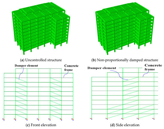
Figure 4.
Finite element structural model in ABAQUS.
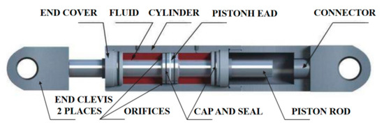
Figure 5.
Viscous damper.

Table 1.
Velocity damper parameters.
Based on the material stress–strain relationship of fiber element models, using the B32 element type, and considering structural geometric non-linearity and material non-linearity, the beam and column models are established, with rebars standardized through steel beam elements with an equal cross-sectional area, and floor slabs are simulated using shell elements. In the structural dynamic analysis, the damping form used is Rayleigh damping.
5.2. Selection of Ground Motions
Strong ground motion records were required to perform reasonable IDA on uncontrolled and damped structures. In this study, the recommended earthquake motion record set is from FEMA P-695 in ATC-63 [45]. Ground motion records were selected from the Earthquake Motion Database of the Pacific Earthquake Engineering Research Center. The selected records included 22 far-field and 28 near-field records (Figure 6). Among the near-field records, there were 14 sets with pulse-like characteristics and 14 sets without pulses.
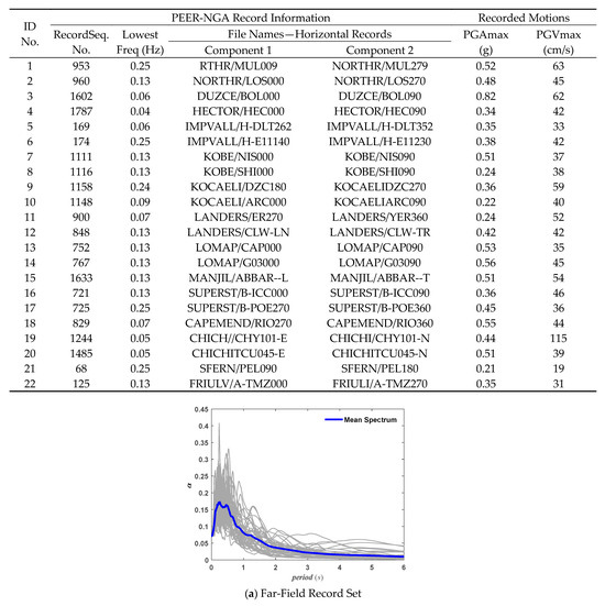
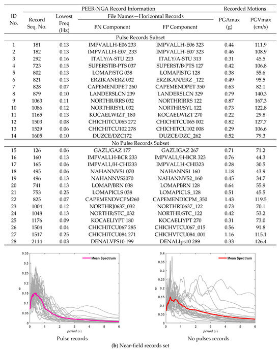
Figure 6.
Seismic records set for FEMA P-695 in ATC-63.
5.3. Complex Modal Analysis
From Figure 7, it can be observed that the first two vibration modes of the non-proportional damping structure are translational, while the third mode is torsional. The corresponding natural periods are T1 = 0.9072 s, T2 = 0.8776 s, and T3 = 0.6812 s, with the ratio of T3 to T1 being 0.75, which is less than 0.9, meeting the requirement of the structure’s stiffness. Compared to the lumped mass model, the three-dimensional structure considers the effects of both translational and torsional deformation.
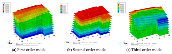
Figure 7.
Complex modal analysis.
5.4. Earthquake Probability Demand Analysis
Performing non-linear IDA on both uncontrolled structures and damped structures, with peak ground acceleration (PGA) ranging from 0.1 g to 1.0 g, the data samples of seismic motion at different levels and the corresponding base shear of the structures are calculated. Power function fitting was then conducted on the data samples to obtain the relationship between the seismic motions.
By fitting the sample data points of uncontrolled and damped structures, as shown in Figure 8, the relationships between X-direction PGA and structural shear force are, respectively, obtained as and , while the relationships between Y-direction PGA and structural shear force are obtained as and . At lower PGA levels, the PGA–shear force curves for uncontrolled structures and damped structures are relatively close. As the PGA increases, the differences between the PGA–shear force curves of the two structures become increasingly pronounced. This occurs because under small seismic actions, the effect of the base isolation devices is relatively minor, and the structural response is primarily determined by the linear stiffness characteristics of the structure itself. As the PGA increases, the non-linear characteristics of the damping devices become more significant during strong seismic actions, effectively suppressing the dynamic response of the structure and leading to a greater disparity in seismic responses between the damped structure and the uncontrolled structure. The PGA-shear force curve of the damped structure typically exhibits a smaller slope compared to that of the uncontrolled structure. This is due to the fact that the damped structure reduces the transmission of seismic forces by increasing the overall stiffness and energy dissipation of the system, thereby achieving optimal energy absorption and dissipation, which results in a relatively mild increase in bottom shear forces. At the same PGA level, the shear force of the damped structure is generally less than that of the uncontrolled structure as the damping devices effectively absorb and dissipate seismic energy, thereby reducing the seismic forces acting on the base of the structure and enhancing its seismic performance. Comparative analysis indicates that the damped structure effectively reduces bottom shear forces under equivalent seismic actions, thereby improving the overall seismic performance of the structure, primarily due to the energy dissipation and stiffness adjustment functions of the damping devices.
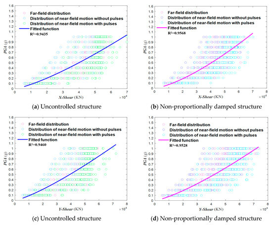
Figure 8.
IDA curve of structural shear force.
By fitting the sample data points of the uncontrolled and damped structures (Figure 9), it can be observed that compared to the uncontrolled structures, the slope of the fitted line for the shear seismic demand in the X-direction of the damped structures decreased by 12.78%, while the slope of the fitted line for the shear seismic demand in the Y-direction of the damped structures decreased by 4.08%. Moreover, compared to the uncontrolled structures, the intercept of the fitted line for the shear seismic demand in the X-direction of the damped structures decreased by 0.31%, whereas the intercept of the fitted line for the shear seismic demand in the Y-direction of the damped structures increased by 0.71%.
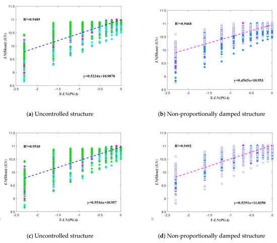
Figure 9.
Seismic probability demand of structural base shear.
By fitting the sample data points of the uncontrolled and damped structures (Figure 10), compared to the uncontrolled structures, the slope of the fitting line for the drift seismic demand of the X-direction damped structures decreased by 0.17%, whereas the slope of the fitted line for the drift seismic demand of the Y-direction damped structures increased by 4.71%. Compared to the uncontrolled structures, the intercept of the fitting line for the drift seismic demand of the X-direction damped structures increased by 8.47%, whereas the intercept of the fitting line for the drift seismic demand of the Y-direction damped structures increased by 3.34%.
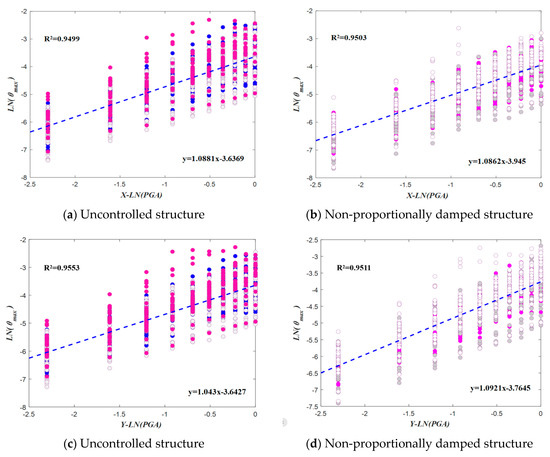
Figure 10.
Seismic probability demand of structural drift.
The three-dimensional analytical model considered the effects of the spatial stiffness and mass distribution of the structure. Under strong earthquake actions, the seismic demands on the inter-story drift and base shear in different directions exhibited significant coupling and interactive effects. By comparing the slopes of the seismic demand fitting lines for the shear demand (Figure 9) and drift demand (Figure 10), it can be observed that the seismic response of the structure to changes in shear demand at the bottom was high, indicating the shear index demonstrates significant sensitivity to seismic demands.
5.5. Fragility Analysis
Based on the analysis of the data, as shown in Figure 11, the shear damage probability curves for the different performance levels of the structures were obtained based on the data analysis. When PGA = 0.4 g, the probability of slight damage in the X-direction for the uncontrolled structure was 47.14%, the probability of exceeding life safety was 3.56%, and the probability of collapse was 0.02%. Therefore, the probabilities of slight damage to the structure, safety of life, and collapse prevention were 52.86%, 43.58%, and 3.58%, respectively. The structure does not collapse or come close to collapse. The probabilities of slight damage in the Y-direction for the uncontrolled structure, exceeding life safety and collapse, were 48.54%, 3.84%, and 0.02%, respectively. Therefore, the probabilities of slight damage to the structure, safety of life, and collapse prevention were 51.46%, 44.72%, and 3.82%, respectively. The structure does not collapse or come close to collapse. When PGA = 0.4 g, the probability of slight damage in the X-direction for the damped structure was 20.54%, the probability of exceeding life safety was 0.53%, and the probability of collapse was 0%. Therefore, the probabilities of slight damage to the structure, safety of life, and collapse prevention were 79.46%, 20.01%, and 0.53%, respectively. The structure does not collapse or come close to collapse. The probability of slight damage in the Y-direction for the damped structure was 20.83%, the probability of exceeding the life safety was 1.05%, and probability of collapse was 0%. Therefore, the probabilities of slight damage to the structure, safety of life, and collapse prevention were 71.69%, 27.25%, and 1.05%, respectively. The structure does not collapse or come close to collapse. Compared with the uncontrolled structure, the probability of exceeding the life safety of the damped structure was reduced by 85.11% in the X-direction and 72.65% in the Y-direction. The structure does not collapse or come close to collapse.
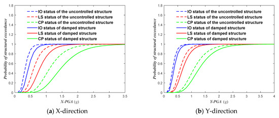
Figure 11.
Fragility curves of structural drift index at different peak ground accelerations (PGAs).
Based on the data analysis, Figure 12 presents the shear damage probability curves for structures with different performance levels. When PGA = 0.4 g, the probability of slight damage in the X-direction for the uncontrolled structure was 55.40%, the probability of exceeding life safety was 13.85%, and the probability of collapse was 1.04%. Therefore, the probabilities of slight damage to the structure, safety of life, and prevention of collapse were 44.60%, 41.55%, and 12.81%, respectively. The structure does not collapse or come close to collapse. The probabilities of slight damage in the Y-direction for the uncontrolled structure, exceeding life safety, and collapse were 53.77%, 13.89%, and 1.17%, respectively. Therefore, the probabilities of slight damage to the structure, safety of life, and prevention of collapse were 46.23%, 39.88%, and 12.72%, respectively. The structure does not collapse or come close to collapse. When PGA = 0.4 g, the probability of slight damage in the X-direction for the damped structure is 38.50%, the probability of exceeding life safety is 5.93%, and the probability of collapse is 0.23%. Therefore, the probabilities of slight damage to the structure, safety of life, and collapse prevention were 61.50%, 32.57%, and 5.7%, respectively. The structure does not collapse or come close to collapse. The probability of slight damage in the Y-direction for the damped structure was 40.45%, the probability of exceeding the life safety was 7.13%, and the probability of collapse was 0.36%. Therefore, the probabilities of slight damage to the structure, safety of life, and collapse prevention were 59.55%, 33.32%, and 6.77%, respectively. The structure does not collapse or come close to collapse. Compared to the uncontrolled structure, the probability of collapse for the damped structure was reduced by 77.88% in the X-direction and 69.23% in the Y-direction.
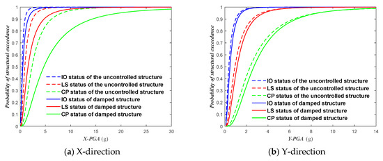
Figure 12.
Fragility curves of base shear index for different peak ground accelerations (PGA) in structures.
The probability of experiencing moderate or high damage to structures during frequent earthquakes (PGA > 0.07 g) is very low. However, the probability of experiencing moderate or high damage gradually increases during rare earthquakes (PGA > 0.4 g). Based on the structural response under different PGAs, it can be observed that the seismic capacity of typical reinforced concrete structures is significantly improved when passive energy dissipation measures are implemented, especially in the X-axis seismic direction, where the damage probability is greatly reduced after adopting energy dissipation measures. At the same PGA level, the fragility curve of ordinary reinforced concrete frame structures is typically steeper. This is because ordinary reinforced concrete structures have limited seismic resistance, and when the PGA reaches a certain level, the structure is prone to severe damage. Damped structures, on the other hand, incorporate devices such as dampers to effectively reduce the impact of earthquakes on the structure. The fragility curve of the damped structures is relatively flatter, allowing the structure to maintain relatively good seismic performance, even at higher PGA levels.
According to the ACT-63 standard [45], there is a recommendation for a collapse probability of 10% as the threshold for evaluating the structural collapse resistance. As shown in Figure 13, when PGA = 0.9 g, the probability of collapse or near-collapse in the X-direction for uncontrolled structures is 10.59%, and in the Y-direction, it is 10.97%. For the damped structures, the probabilities of collapse or near-collapse in the X- and Y-directions were 2.89% and 6.12%, respectively. Compared with uncontrolled structures, the life-safety surpass probability of damped structures was reduced by 72.71% in the X-direction and 44.21% in the Y-direction. As shown in Figure 14, when PGA = 1.0 g, the probability of collapse or near-collapse in the X-direction for uncontrolled structures is 14.80%, and in the Y-direction, it is 14.27%. For the damped structures, the probabilities of collapse or near-collapse in the X- and Y-directions were 4.28% and 7.50%, respectively. Compared with uncontrolled structures, the life-safety surpass probability of damped structures was reduced by 71.08% in the X-direction and 47.44% in the Y-direction.
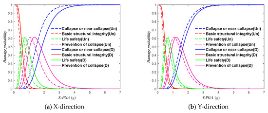
Figure 13.
Damage probability of structural drift index under different performance levels.
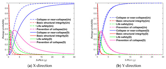
Figure 14.
Damage probability of structural base shear index under different performance levels.
Under rare seismic events, the collapse probability of uncontrolled and damped structures decreases with the increase in seismic intensity. When considering structural drift as an indicator, the life-safety surpass probability for uncontrolled structures was 0.02%, whereas for damped structures, it was 0. When considering base shear as an indicator under rare seismic events, the life-safety surpass probability for uncontrolled structures ranges from 1.04% to 1.17%, whereas that for damped structures, it ranges from 0.23% to 0.36%. These probabilities are all lower than the threshold value set in ACT-63, which suggests the use of a collapse probability of less than 10% as an evaluation criterion for structural collapse resistance under rare seismic events [46]. This indicates that the collapse resistance capacity of damped structures in the 8-degree designated seismic zone is adequate, and there is no need to take measures to enhance their collapse resistance capacity.
5.6. Different Limit State Performance Points
The bottom shear limit of a structure corresponding to different limit states can be obtained by fitting the data according to the drifts corresponding to the different limit states.
From Table 2, the ratios of severe damage LS, complete collapse CP, and moderate damage IO in the limit state fragility analysis based on structural shear force are 1.6 and 2.6, respectively. In comparison, there were differences in the ratios of severe damage, complete collapse, and moderate damage in the limit state fragility analysis based on the structural drift index, which were 2.0 and 4.0. This is because the indicators used in the fragility analyses based on structural shear force and structural drift are different. Fragility analysis based on the structural shear force mainly focuses on the magnitude of the shear force, which is the internal force of the structure. A fragility analysis based on structural drift focuses on the overall degree of deformation of the structure, which is the angular displacement of the structure. The results of the shear force fragility analysis often show higher levels of severe damage or complete damage and lower levels of moderate damage, resulting in smaller ratios. In shear force fragility analysis, factors such as the shear resistance, stiffness, and strength of the structure are mainly considered in relation to structural damage. Drift fragility analysis, on the other hand, places more emphasis on factors such as flexibility, deformation capacity, and the seismic performance of the structure. The results of the drift fragility analysis usually show higher levels of moderate displacement, resulting in smaller ratios compared with severe damage or complete damage levels. This difference does not mean that one analysis method is more accurate than the other; rather, the evaluation indicators focused on by the two methods differ and are applicable to different engineering requirements and objectives. In practical applications, multiple fragility indicators are commonly considered to comprehensively evaluate the seismic performance of a structure.
Table 2.
Comparison of shear force ratio coefficients for different performance points.
From the different analysis states, the ratios of the shear force to the multi-seismic shear force of the uncontrolled structure in the X-direction at the limit states of moderate damage, severe damage, and complete damage were 8.78, 14.31, and 23.35, respectively, with a multi-seismic shear force of 3912.70 KN. The corresponding ratios in the Y-direction (with a shear force of 3912.70 KN) were 8.83, 14.16, and 22.70, respectively. In the X-direction, the ratios of the shear force to the multi-seismic shear force of the damped structure at the limit states of moderate damage, severe damage, and complete damage were 10.22, 16.98, and 28.19, respectively, with a multi-seismic shear force of 4110.30 KN. The corresponding ratios In the Y-direction (with a shear force of 4110.30 KN) were 9.64, 15.73, and 25.67, respectively. Specifically, the ratios of shear force to multi-seismic shear force at the limit states of moderate, severe, and complete damage for the uncontrolled structure were 8.80, 14.24, and 23.02, respectively. For the damped structure, the corresponding ratios are 9.93, 16.35, and 26.93. Compared with the various limit states of the uncontrolled structure, the damped structure exhibited improvement percentages of 12.79%, 14.86%, and 16.97% for the limit states of moderate, severe, and complete damage, respectively.
Table 2 shows that the incorporation of dampers into the structure led to varying degrees of enhancement in the limit states. In the X-direction, the ratios of the corresponding states of moderate damage, severe damage, and complete damage to the uncontrolled structures for the dampened structure based on shear fragility analysis were 1.22, 1.25, and 1.27, respectively. In the Y-direction, the ratios of the corresponding states of moderate damage, severe damage, and complete damage to the non-controlled structures for the dampened structure based on shear fragility analysis were 1.15, 1.17, and 1.19, respectively.
5.7. Median and Logarithmic Standard Deviation of Fragility Functions
The median values of the fragility functions for the uncontrolled and damped structures in terms of immediate occupancy (IO), life safety (LS), and collapse prevention (CP) exhibited an increasing trend with higher limit states. The median shear values are consistently higher for uncontrolled structures than for damped structures. As shown in Figure 15, uncontrolled structures have lower stiffness than damped structures, resulting in larger deformations and shear responses under seismic actions. Damped structures, on the other hand, incorporate seismic devices or techniques that effectively reduce structural deformations and mitigate seismic responses, thus resulting in relatively smaller median shear values. Damped structures typically possess a better energy dissipation capacity, enabling them to absorb more energy during earthquakes and reduce shear responses. By contrast, ordinary reinforced concrete frame structures exhibit relatively weaker performances and are susceptible to direct impacts from seismic forces, leading to larger median shear values. The smaller median shear values for ordinary reinforced concrete frame structures compared with damped structures in the fragility functions may be attributed to differences in structural stiffness, energy dissipation capacity, and design concepts.
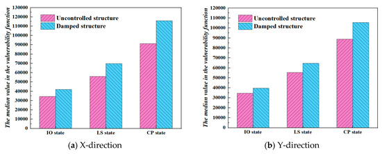
Figure 15.
Comparison of median values of fragility functions for different structural shear forces.
A statistical analysis was performed on the data, as shown in Figure 16. For the ordinary reinforced concrete frame structure, the logarithmic standard deviations of the seismic shear demands at the immediate occupancy (IO) and life safety (LS) performance levels were higher than those of the non-proportionally damped structure. However, at the collapse prevention (CP) performance level, the shear standard deviation of the ordinary frame was lower than that of the non-proportionally damped structure. This indicated that the non-proportional damping structure exhibited greater response variability and dispersion at the CP performance level, suggesting higher uncertainty in the structural behavior when approaching the limit state. In contrast, the ordinary frame structure showed higher dispersion at the lower damage states (IO and LS) but more reliable and stable performance at the CP limit state. Specifically, the non-proportional damping structure incorporated viscous dampers to enhance its seismic energy dissipation capacity. At the CP performance level, corresponding to structural responses near collapse, the activation of the non-linear damping mechanism in the structure under large displacements, along with the potential involvement of higher-mode effects and other non-linear deformation modes, introduced increased uncertainty in the structural response of the non-proportional damping system at the CP level. This high degree of response scatter was reflected in the significantly increased logarithmic standard deviations observed in the statistical data.
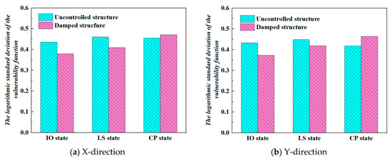
Figure 16.
Comparison of standard deviations of fragility functions for different structural shear forces.
6. Conclusions
In this study, non-proportional damping was extended to a three-dimensional non-proportional damping structure, and the dynamic response of the three-dimensional structure was analyzed through large-scale general finite element analysis. A structural seismic performance evaluation method that utilizes the structural shear fragility index to calculate the collapse probability was proposed. The limit performance states of the structure were determined based on the ratio of the bottom shear force, and the corresponding shear values were predicted for the moderate damage (IO), severe damage (LS), and complete damage (CP) states; this index was used to further determine whether the underlying structure has brittle failure.
By establishing a three-dimensional matrix element for viscous dampers and utilizing the Fortran language for the secondary development of the ABAQUS software, a VUEL damper element subroutine for dynamic explicit elastoplastic calculations of viscous dampers was developed. The VUEL program accurately calculated the forces, displacements, and energy dissipations of the dampers. This study provided an analytical tool for evaluating the performance of structures equipped with viscous dampers under dynamic loading conditions. This offers an effective approach for assessing the seismic differences between uncontrolled and damped structures. In this study, an analysis tool was developed to analyze the structural performance of structures equipped with viscous dampers under dynamic loading conditions. This approach was also used in this study to effectively evaluate the seismic differences between uncontrolled and damped structures.
Using Python programs, an IDA analysis program was developed for ABAQUS software. The recommended far-field and near-field earthquake record sets from FEMAP-695 in ATC-63 were utilized to perform numerical fragility analyses of both the uncontrolled and seismically damped structures. The ratios of the limit performance states for moderate damage (IO), severe damage (LS), and complete damage (CP) in the uncontrolled structure were 1:1.6:2.6. The seismic performance improvement of the damped structures compared to the various limit performance states of the uncontrolled structures was found to be 12.79%, 14.86%, and 16.97% for the moderate, severe, and complete damage limit states, respectively.
The shear-to-frequent earthquake shear ratios for the limit states of moderate damage (IO), severe damage, and complete damage (CP) in the uncontrolled structures were 8.80, 14.24, and 23.02, respectively. For the damped structures, the corresponding ratios are 9.93, 16.35, and 26.93. The median values of the fragility functions for moderate damage (IO), severe damage, and complete damage (CP) in both uncontrolled and damped structures increased with an increase in the limit states. For the uncontrolled structures, the logarithmic standard deviation of shear was higher for the IO and LS than for the damped structures. However, during the complete damage (CP) stage, the shear standard deviation of the uncontrolled structures was lower than that of the damped structures. Based on the results of the shear fragility analysis, the ratios of severe and complete damage to moderate damage were lower than those obtained from the drift fragility analysis. In addition, a hysteresis phenomenon was observed in the fragility curves of the bottom shear force. These two analytical methods focus on different evaluation indicators and are applicable to different engineering requirements and objectives.
Author Contributions
Conceptualization, J.W., T.H., X.H. and F.Z.; Methodology, J.W., T.H. and X.H.; Software, J.W., T.H. and X.H.; Validation, J.W., T.H. and X.H.; Writing—original draft, J.W., T.H. and X.H.; Writing—review & editing, J.W., T.H. and X.H.; Supervision, P.T. All authors have read and agreed to the published version of the manuscript.
Funding
Thanks to the following funding projects: the National Key Research and Development Program (2021YFC3100701), the National Natural Science Foundation of China Project (52378292), and the Research Project of Baoshan University (Grant No. 22BYZY03).
Data Availability Statement
The data presented in this study are available in the article.
Conflicts of Interest
The authors declare no conflicts of interest.
References
- Zuo, H.; Zhu, S. Bistable track nonlinear energy sinks with nonlinear viscous damping for impulsive and seismic control of frame structures. Eng. Struct. 2022, 272, 114982. [Google Scholar] [CrossRef]
- Fathizadeh, S.F.; Dehghani, S.; Yang, T.Y.; Noroozinejad Farsangi, E.; Vosoughi, A.R.; Hajirasouliha, I.; Takewaki, I.; Malaga-Chuquitaype, C.; Varum, H. Trade-off Pareto optimum design of an innovative curved damper truss moment frame considering structural and non-structural objectives. Structures 2020, 28, 1338–1353. [Google Scholar] [CrossRef]
- Zhang, C.; Li, Z.; Huang, W.; Deng, X.; Gao, J. Seismic performance of semi-rigid steel frame infilled with prefabricated damping wall panels. J. Constr. Steel Res. 2021, 184, 106797. [Google Scholar] [CrossRef]
- Zhou, L.; Li, X.; Yan, Q.; Li, S. Blast test and probabilistic vulnerability assessment of a shallow buried RC tunnel considering uncertainty. Int. J. Impact Eng. 2023, 180, 104717. [Google Scholar] [CrossRef]
- Sonda, D.; Pollini, A.V. SISMO-Fast: Energy-based method for rapid seismic vulnerability assessment of industrial precast RC buildings. Procedia Struct. Integr. 2023, 44, 115–122. [Google Scholar] [CrossRef]
- Wu, Y.; Meng, B.; Wang, L.; Qin, G. Seismic vulnerability analysis of buried polyethylene pipeline based on finite element method. Int. J. Press. Vessel. Pip. 2020, 187, 104167. [Google Scholar] [CrossRef]
- Ouyang, X.; Zhang, Y.; Ou, X.; Shi, Y.; Liu, S.; Fan, J. Seismic fragility analysis of buckling-restrained brace-strengthened reinforced concrete frames using a performance-based plastic design method. Structures 2022, 43, 338–350. [Google Scholar] [CrossRef]
- Fontenele, A.; Campos, V.; Matos, A.M.; Mesquita, E. A vulnerability index formulation for historic facades assessment. J. Build. Eng. 2023, 64, 105552. [Google Scholar] [CrossRef]
- Alothman, A.; Mangalathu, S.; Hashemi, J.; Al-Mosawe, A.; Alam, M.D.M.; Allawi, A. The effect of ground motion characteristics on the fragility analysis of reinforced concrete frame buildings in Australia. Structures 2021, 34, 3583–3595. [Google Scholar] [CrossRef]
- Zhang, Z.; Zhan, Y.; Shen, H.; Qian, H.; Sheng, P. Seismic performance of self-centering braced rocking frame with novel self-centering friction dampers characterized by low-secondary stiffness. Structures 2023, 57, 105225. [Google Scholar] [CrossRef]
- Barbagallo, F.; Bosco, M.; Ghersi, A.; Marino, E.M. An over-damped multimodal adaptive nonlinear static analysis for seismic assessment of infilled RC buildings. Eng. Struct. 2021, 229, 111622. [Google Scholar] [CrossRef]
- Khanmohammadi, M.; Eshraghi, M.; Ghafarian Mashhadinezhad, M.; Sayadi, S.; Zafarani, H. Post-earthquake seismic assessment of residential buildings following Sarpol-e Zahab (Iran) earthquake (Mw7.3)—Part 2: Seismic vulnerability curves using quantitative damage index. Soil. Dyn. Earthq. Eng. 2023, 173, 108120. [Google Scholar] [CrossRef]
- Hou, J.; Lu, J.; Chen, S.; Li, N. Study of seismic vulnerability of steel frame structures on soft ground considering group effect. Structures 2023, 56, 104934. [Google Scholar] [CrossRef]
- Liu, G.; Geng, P.; Wang, T.; Meng, Q.; Huo, F.; Wang, X.; Wang, J. Seismic vulnerability of shield tunnels in interbedded soil deposits: Case study of submarine tunnel in Shantou Bay. Ocean Eng. 2023, 286, 115500. [Google Scholar] [CrossRef]
- Wang, Y.; Yang, F.; Yang, J.-S.; Tong, L.-L.; Li, S.; Liu, Q.; Hou, G.-L.; Sun, P.-D.; Xing, M.; Zheng, G. Study on vibration damping performance of a petal-shaped seismic metamaterial. Structures 2023, 56, 104898. [Google Scholar] [CrossRef]
- Kim, J.; Lorenzoni, F.; Salvalaggio, M.; Valluzzi, M.R. Seismic vulnerability assessment of free-standing massive masonry columns by the 3D Discrete Element Method. Eng. Struct. 2021, 246, 113004. [Google Scholar] [CrossRef]
- Mazza, F. Displacement-based seismic design of hysteretic damped braces for retrofitting in-plan irregular r.c. framed structures. Soil Dyn. Earthq. Eng. 2014, 66, 231–240. [Google Scholar] [CrossRef]
- Moon, K.H.; Han, S.W.; Lee, C.S. Seismic retrofit design method using friction damping systems for old low- and mid-rise regular reinforced concrete buildings. Eng. Struct. 2017, 146, 105–117. [Google Scholar] [CrossRef]
- Di, F.; Sun, L.; Chen, L.; Zou, Y.; Qin, L.; Huang, Z. Frequency and damping of hybrid cable networks with cross-ties and external dampers: Full-scale experiments. Mech. Syst. Signal Process. 2023, 197, 110397. [Google Scholar] [CrossRef]
- Guo, L.; Wang, J.; Wang, W.; Wang, H. Performance-based seismic design and vulnerability assessment of concrete frame retrofitted by metallic dampers. Structures 2023, 57, 105073. [Google Scholar] [CrossRef]
- Adhikari, S. On the quantification of damping model uncertainty. J. Sound Vib. 2007, 306, 153–171. [Google Scholar] [CrossRef]
- Nia, E.M.; Ling, L.; Awang, M.; Emamian, S.S. (Eds.) Advances in Civil Engineering Materials. In Proceedings of the Selected Articles from the 6th International Conference on Architecture and Civil Engineering (ICACE 2022), Kuala Lumpur, Malaysia, 18–20 August 2022; Springer Nature Singapore: Singapore, 2023; Volume 310. [Google Scholar] [CrossRef]
- Lemos, J.V.; Sarhosis, V. Dynamic analysis of masonry arches using Maxwell damping. Structures 2023, 49, 583–592. [Google Scholar] [CrossRef]
- Sun, L.; Sun, J.; Nagarajaiah, S.; Chen, L. Inerter dampers with linear hysteretic damping for cable vibration control. Eng. Struct. 2021, 247, 113069. [Google Scholar] [CrossRef]
- Jin, Y.; Zhao, Z.; Yang, T. Dynamics of nonlinear energy sink with a polynomial damped frequency converter. Int. J. Non-Linear Mech. 2024, 158, 104565. [Google Scholar] [CrossRef]
- Meng, J.; Sun, D. Research on the Multilayer Free Damping Structure Design. Shock. Vib. 2018, 2018, 6529571. [Google Scholar] [CrossRef]
- Hu, X.; Fang, G.; Ge, Y. Uncertainty propagation of flutter derivatives and structural damping in buffeting fragility analysis of long-span bridges using surrogate models. Struct. Saf. 2024, 106, 102410. [Google Scholar] [CrossRef]
- He, H.; Tan, P.; Hao, L.; Xu, K.; Xiang, Y. Optimal design of tuned viscous mass dampers based on effective damping ratio enhancement effect. J. Sound Vib. 2022, 534, 117018. [Google Scholar] [CrossRef]
- Mourlas, C.; Khabele, N.; Bark, H.A.; Karamitros, D.; Taddei, F.; Markou, G.; Papadrakakis, M. Effect of Soil–Structure Interaction on Nonlinear Dynamic Response of Reinforced Concrete Structures. Int. J. Struct. Stab. Dyn. 2020, 20, 2041013. [Google Scholar] [CrossRef]
- Vanshaj, K.; Shukla, A.K.; Shukla, M. Seismic Response on Soil–Structure Interaction of Asymmetric Plan Buildings with Active Tuned Mass Dampers. Int. J. Struct. Stab. Dyn. 2022, 22, 2250102. [Google Scholar] [CrossRef]
- Zhao, Z.; Hu, X.; Chen, Q.; Yang, K.; Liao, C.; Zhang, R. Negative stiffness-enhanced seismic damping technology for an over-track complex with concrete-encased steel columns. J. Build. Eng. 2023, 73, 106722. [Google Scholar] [CrossRef]
- Chen, L.; Liu, Z.; Zou, Y.; Wang, M.; Nagarajaiah, S.; Sun, F.; Sun, L. Practical negative stiffness device with viscoelastic damper in parallel or series configuration for cable damping improvement. J. Sound Vib. 2023, 560, 117757. [Google Scholar] [CrossRef]
- Karthik Reddy, K.S.K.; Veggalam, S.; Somala, S.N. Spatial variation of structural fragility due to supershear earthquakes. Structures 2022, 44, 389–403. [Google Scholar] [CrossRef]
- Wang, M.; Du, X.-L.; Sun, F.-F.; Nagarajaiah, S.; Li, Y.-W. Fragility analysis and inelastic seismic performance of steel braced-core-tube frame outrigger tall buildings with passive adaptive negative stiffness damped outrigger. J. Build. Eng. 2022, 52, 104428. [Google Scholar] [CrossRef]
- Habieb, A.B.; Valente, M.; Milani, G. Effectiveness of different base isolation systems for seismic protection: Numerical insights into an existing masonry bell tower. Soil Dyn. Earthq. Eng. 2019, 125, 105752. [Google Scholar] [CrossRef]
- Tian, H.; Li, S.; Cui, X. Development of element model subroutines for implicit and explicit analysis considering large deformations. Adv. Eng. Softw. 2020, 148, 102805. [Google Scholar] [CrossRef]
- Giner, E.; Sukumar, N.; Tarancón, J.E.; Fuenmayor, F.J. An Abaqus implementation of the extended finite element method. Eng. Fract. Mech. 2009, 76, 347–368. [Google Scholar] [CrossRef]
- Chopra, A.K. Dynamics of Structures: Theory and Applications to Earthquake Engineering, 5th ed.; Pearson: Hoboken, NJ, USA, 2017. [Google Scholar]
- ABAQUS Inc. Abaqus Analysis User’s Guide; ABAQUS 6.14 HTML Documentation; ABAQUS Inc.: Palo Alto, CA, USA, 2014. [Google Scholar]
- ABAQUS Inc. Abaqus User Subroutines Reference Guide; ABAQUS 6.14 HTML Documentation; ABAQUS Inc.: Palo Alto, CA, USA, 2014. [Google Scholar]
- ABAQUS Inc. Abaqus Theory Guide; ABAQUS 6.14 HTML Documentation; ABAQUS Inc.: Palo Alto, CA, USA, 2014. [Google Scholar]
- Filiatrault, A.; Léger, P.; Tinawi, R. On the computation of seismic energy in inelastic structures. Eng. Struct. 1994, 16, 425–436. [Google Scholar] [CrossRef]
- Dagang, L.V.; Xiaohui, Y.U. Theoretical study of probabilistic seismic risk assessment based on analytical functions of seismic fragility. J. Build. Struct. 2013, 34, 41–48. [Google Scholar]
- Yu, X.-H. Probabilistic Seimic Fragility and Risk Analysis of Reinforced Concrete Frame Structures. Ph.D. Thesis, Harbin Institute of Technology, Harbin, China, 2012. [Google Scholar]
- FEMA 273; Guidelines to the Seismic Rehabilitation of Existing Buildings. Federal Emergency Management Agency: Washington, DC, USA, 1997.
- Applied Technology Council. Quantification of Building Seismic Performance Factors; US Department of Homeland Security: Washington, DC, USA, 2009.
Disclaimer/Publisher’s Note: The statements, opinions and data contained in all publications are solely those of the individual author(s) and contributor(s) and not of MDPI and/or the editor(s). MDPI and/or the editor(s) disclaim responsibility for any injury to people or property resulting from any ideas, methods, instructions or products referred to in the content. |
© 2024 by the authors. Licensee MDPI, Basel, Switzerland. This article is an open access article distributed under the terms and conditions of the Creative Commons Attribution (CC BY) license (https://creativecommons.org/licenses/by/4.0/).