
Influence of Boundary Conditions on the Estimation of Thermal Properties in Insulated Building Walls


Abstract
1. Introduction
2. Experimental Facility and Boundary Conditions
2.1. Case Study

2.2. Experimental Setup
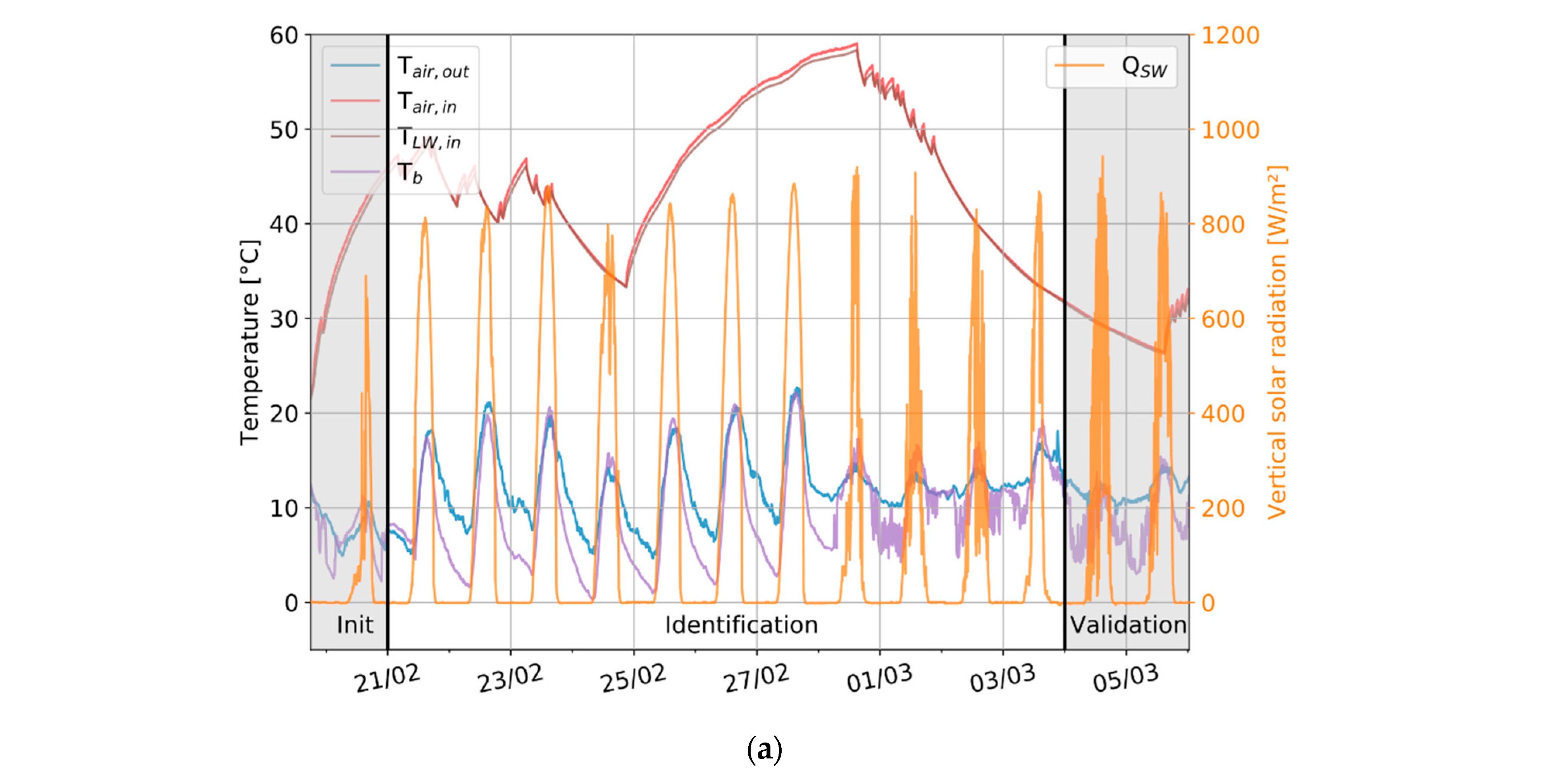
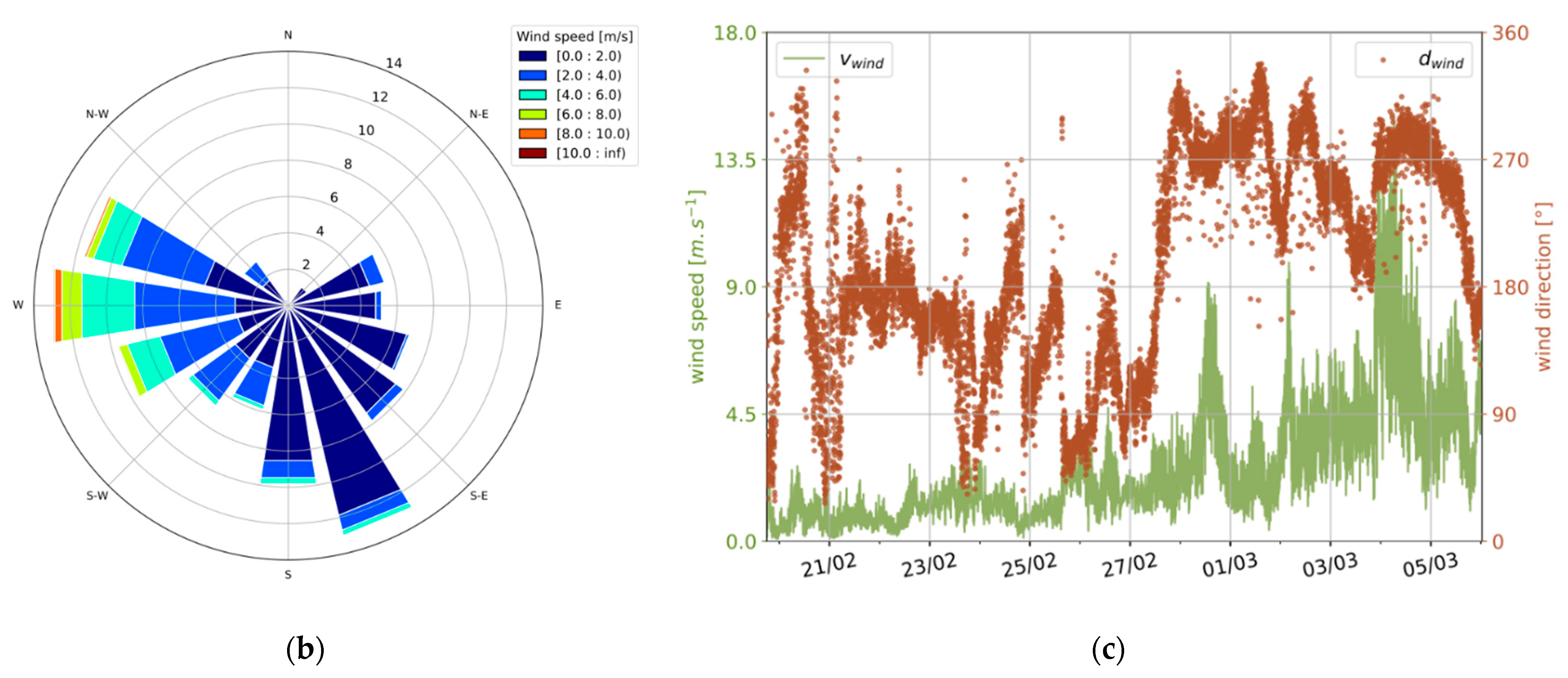
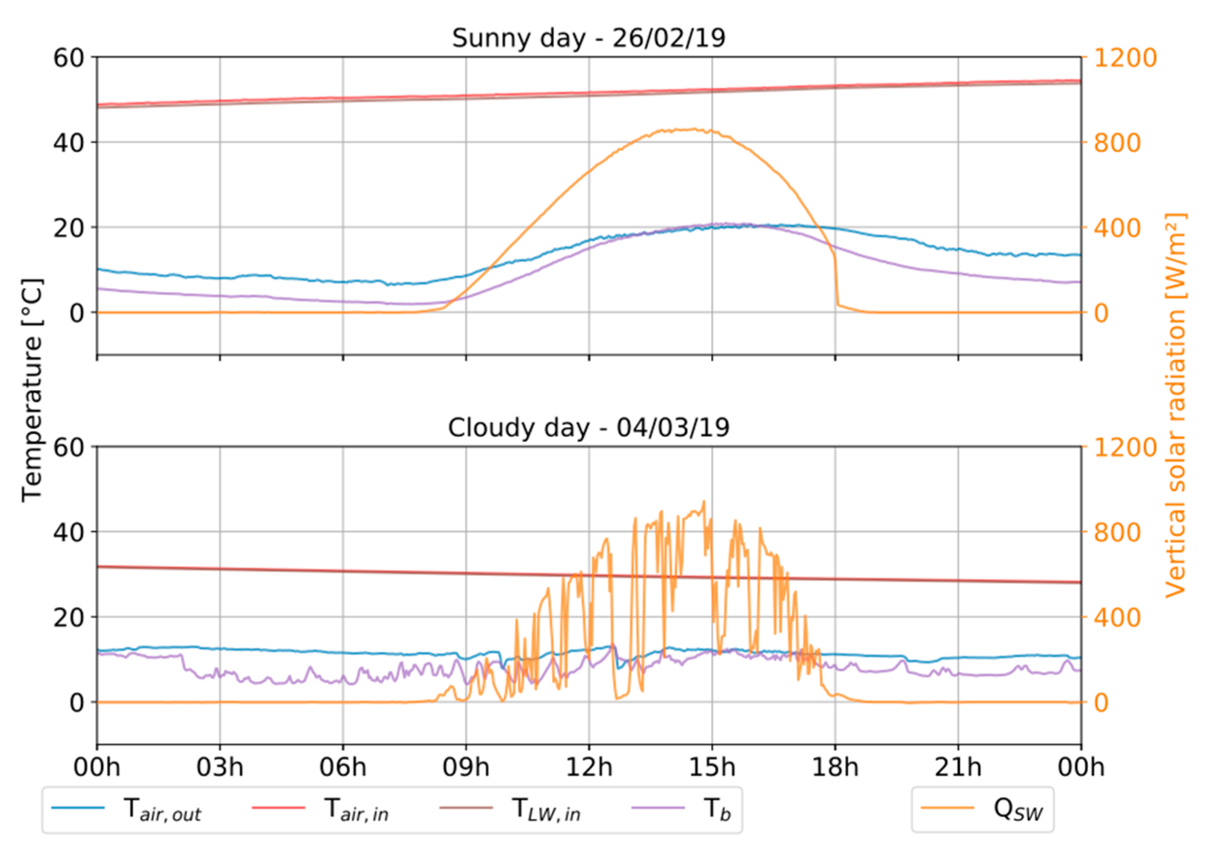
2.3. Experimental Boundary Conditions Measurement
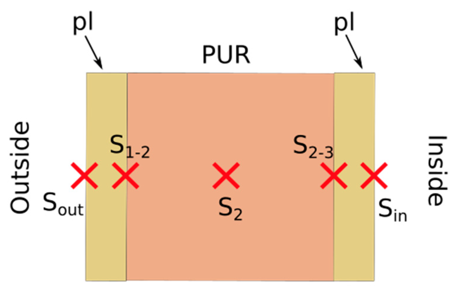
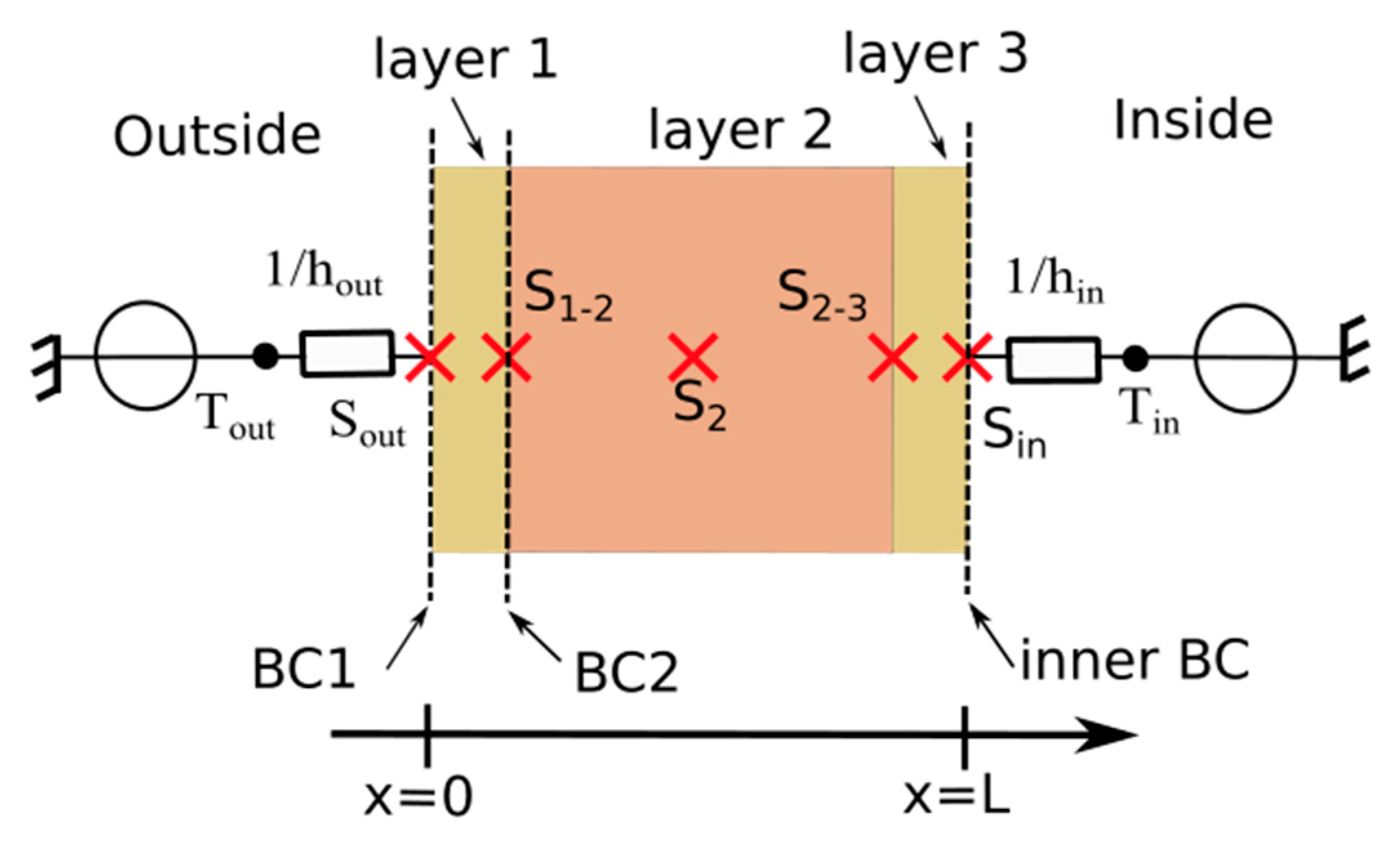
2.4. Exact Location of Sensors Inside the Wall
3. Modelling
3.1. Boundary Conditions
3.2. Heat Transfer Coefficients
3.3. The Reference Model
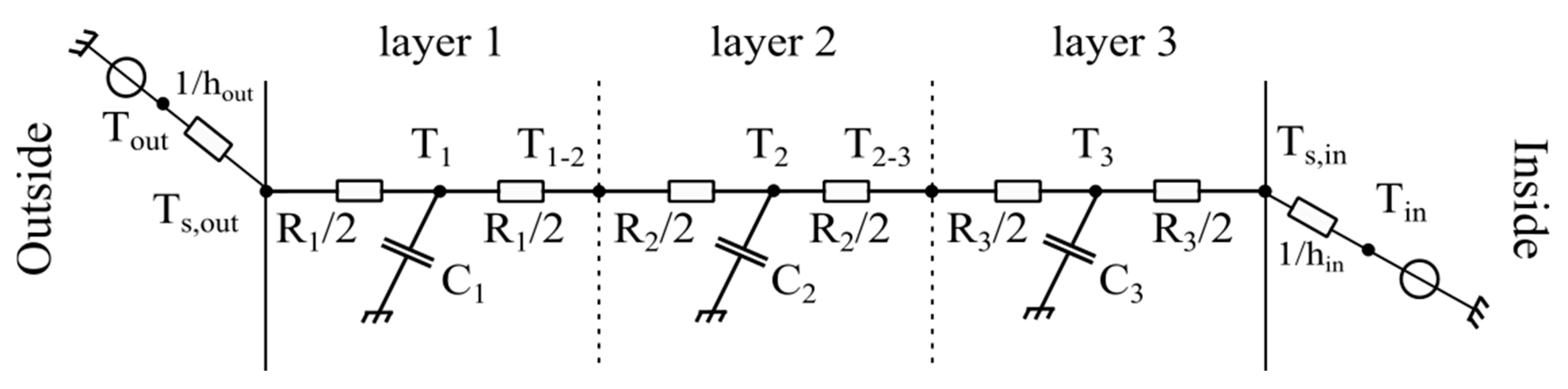
3.4. The Resistance–Capacitance Model
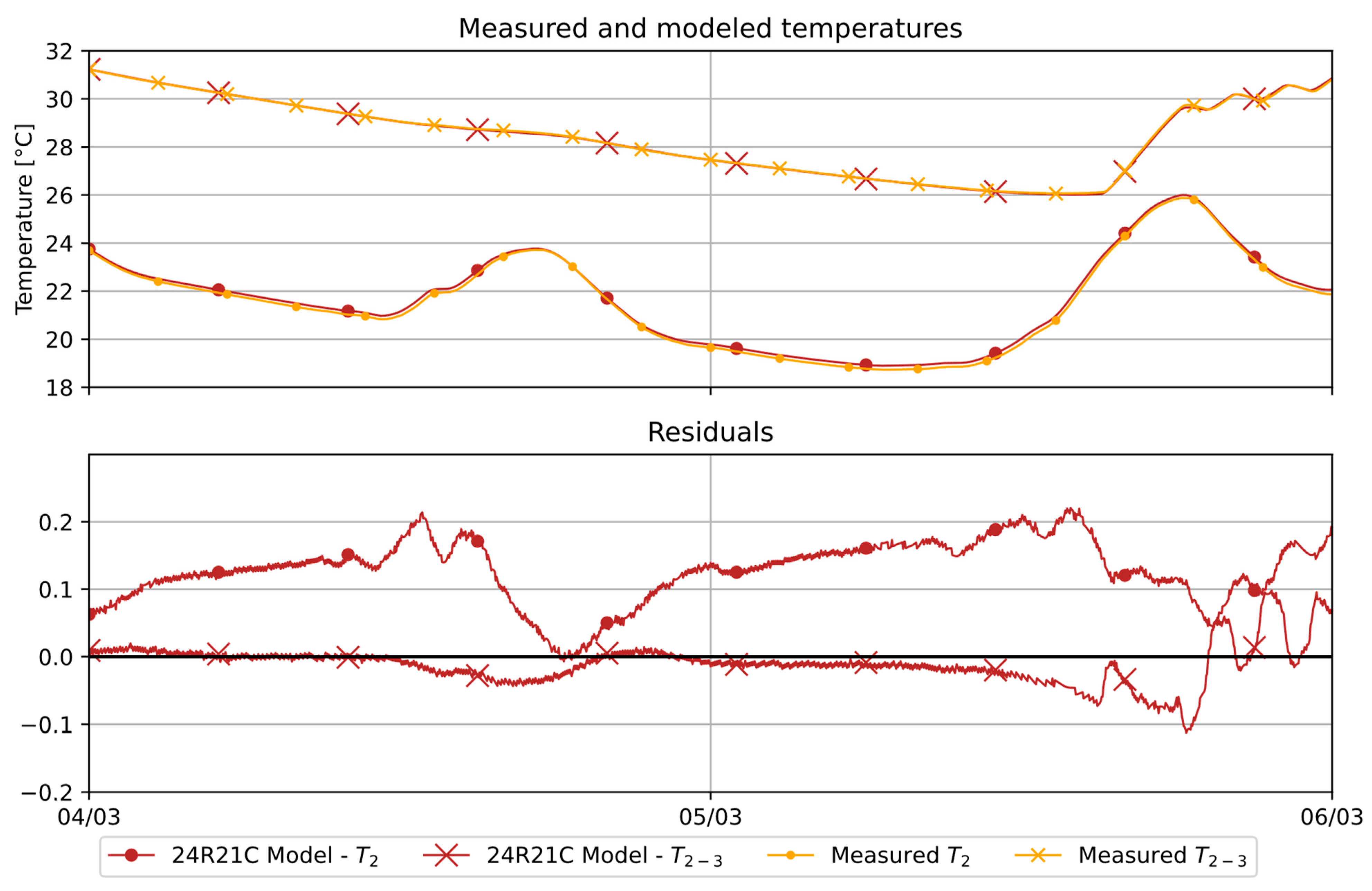
3.5. Model Validation
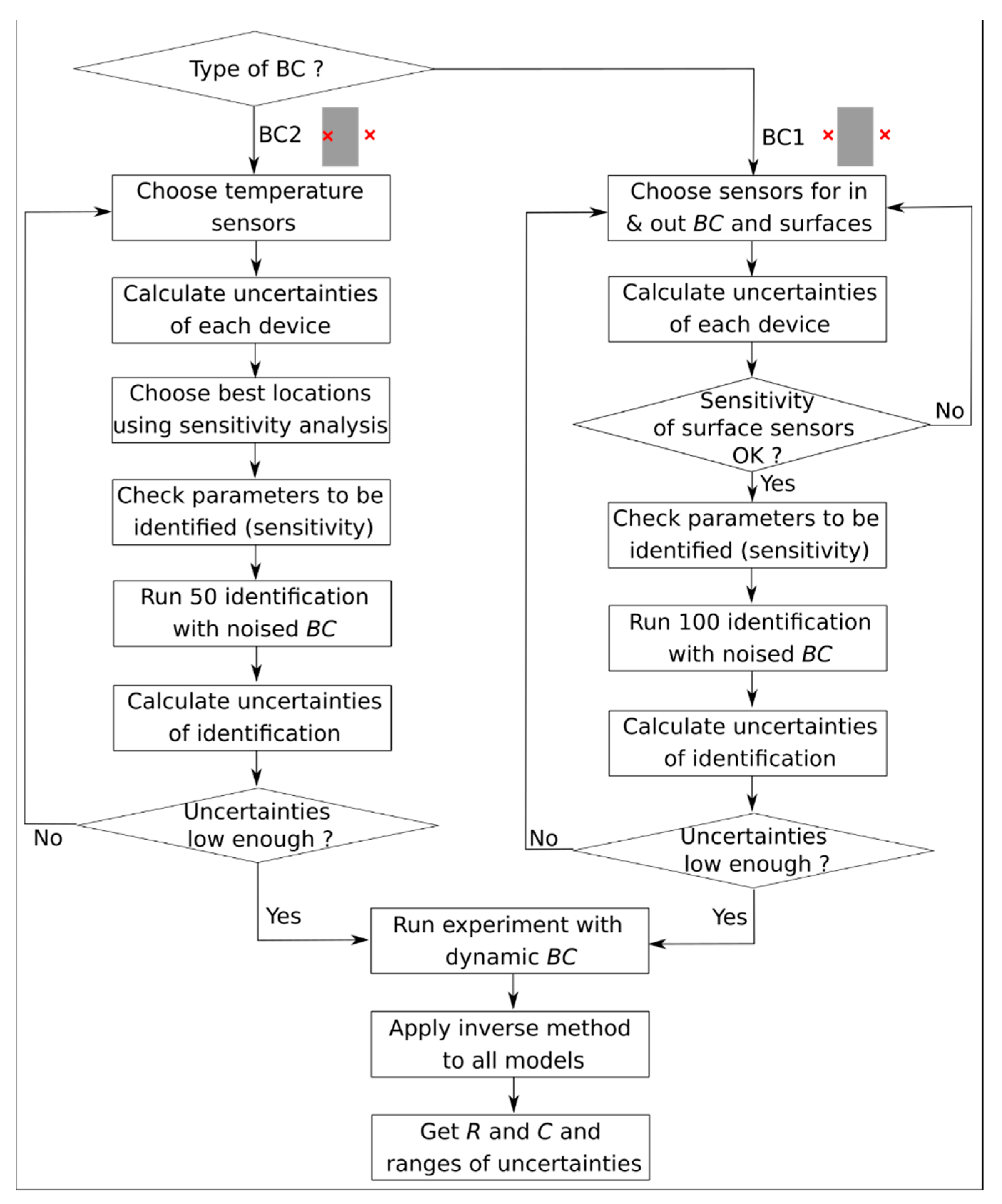
4. Identification Technique
4.1. Principle of the Inverse Method
4.2. Calculation of Uncertainties
5. Results
5.1. Application to Synthetic Data
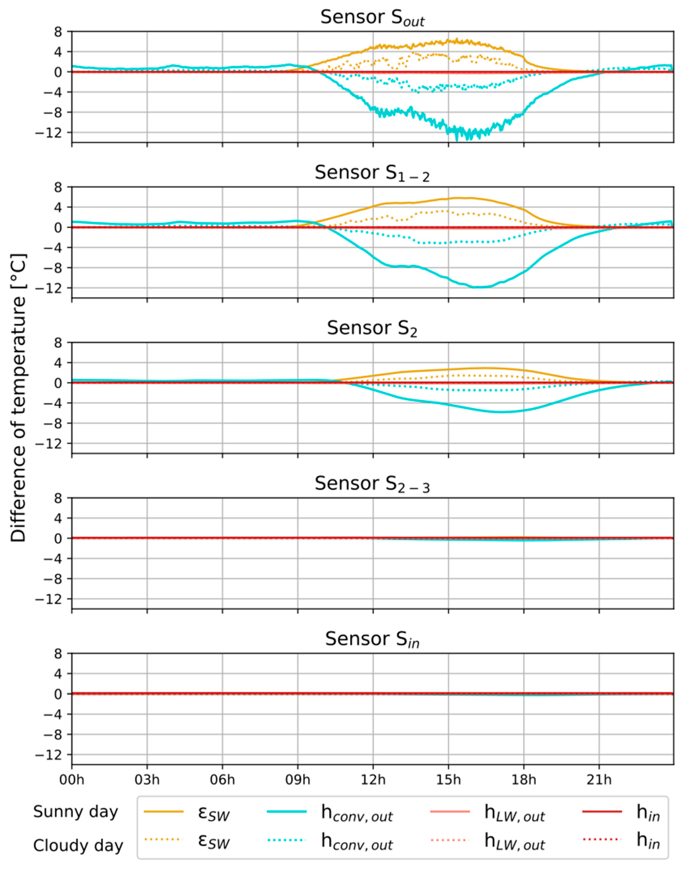
5.1.1. Influence of the Heat Transfer Coefficients and Absorptivity
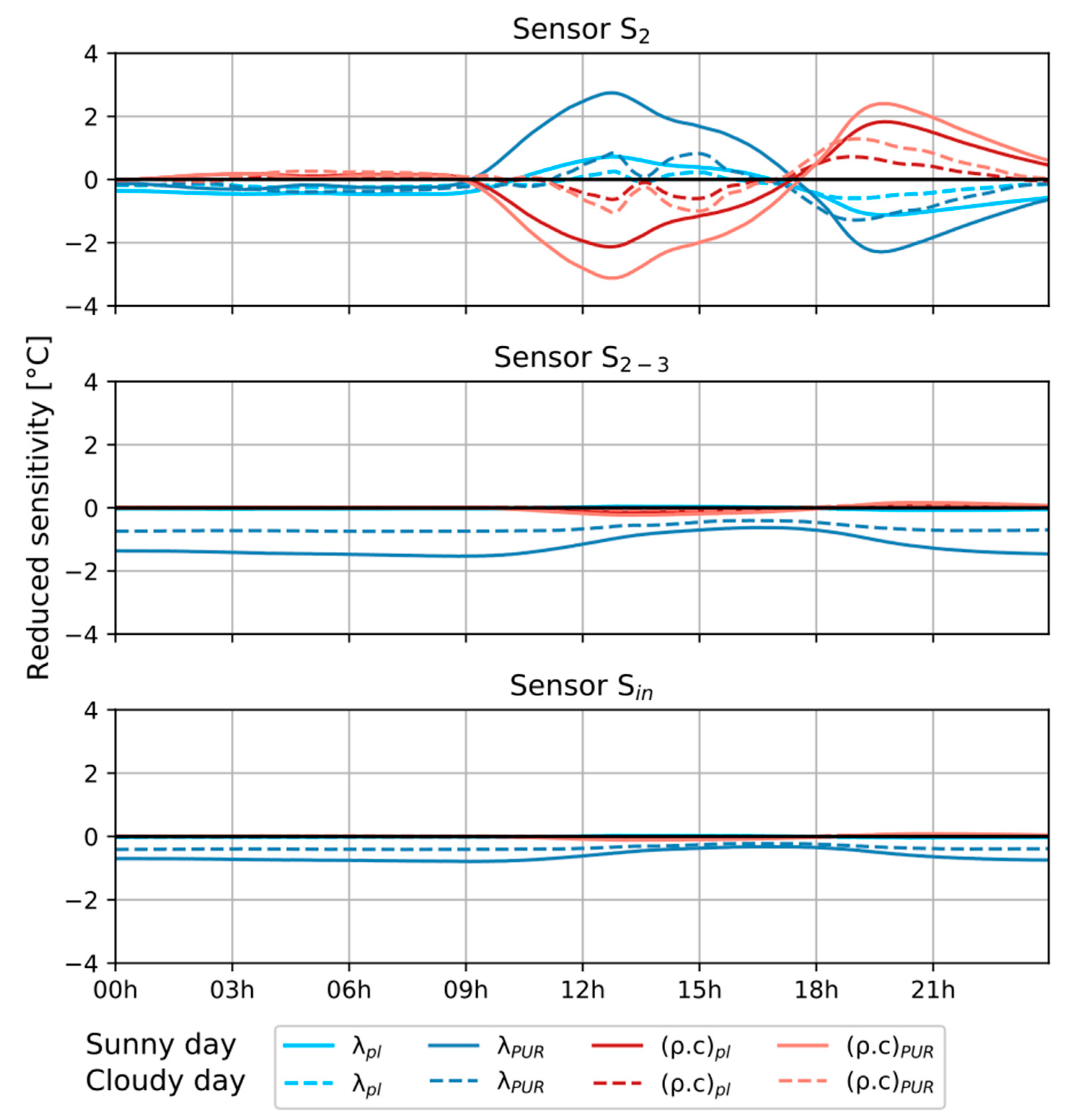
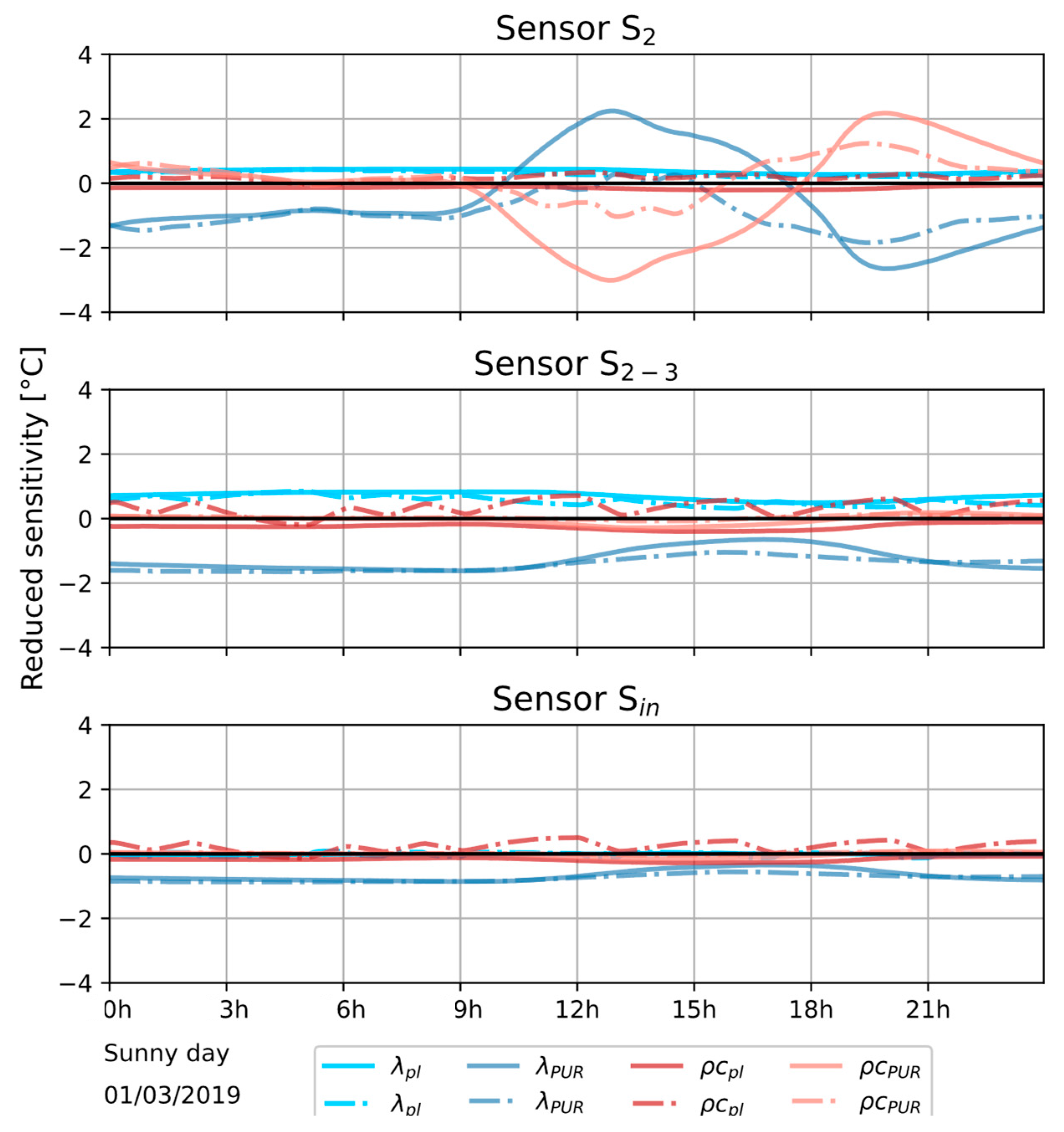
5.1.2. Sensitivity According to Parameters to Be Identified
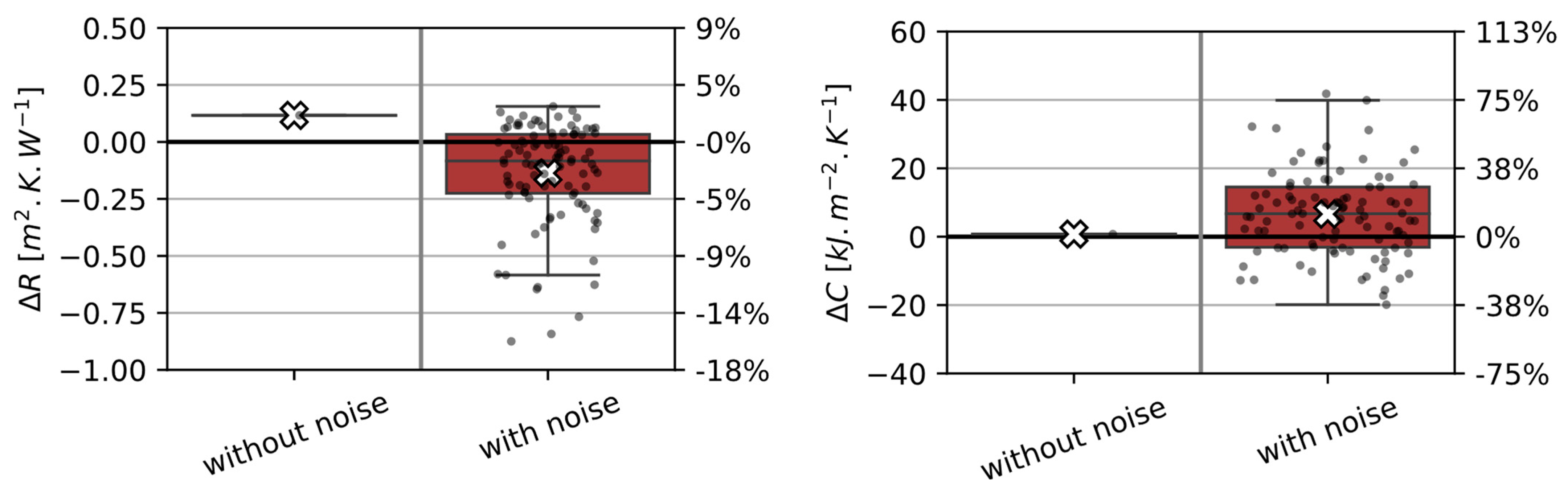
5.1.3. Identification Results with Synthetic Data and Boundary Conditions BC1
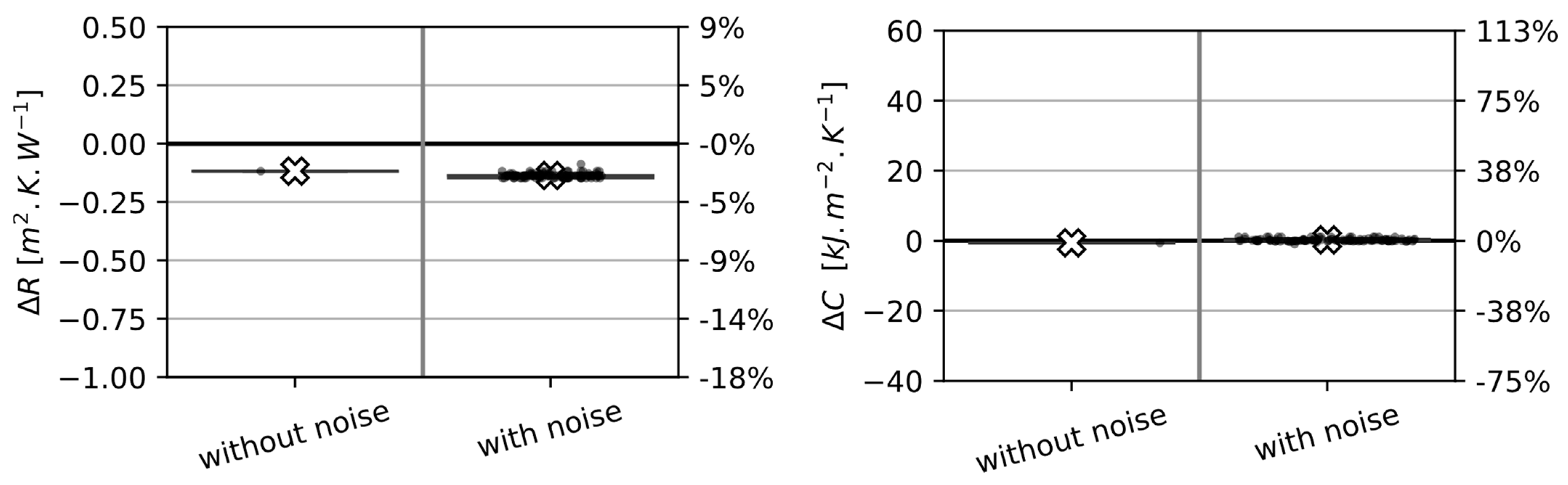
5.1.4. Application to Synthetic Data with Boundary Conditions BC2
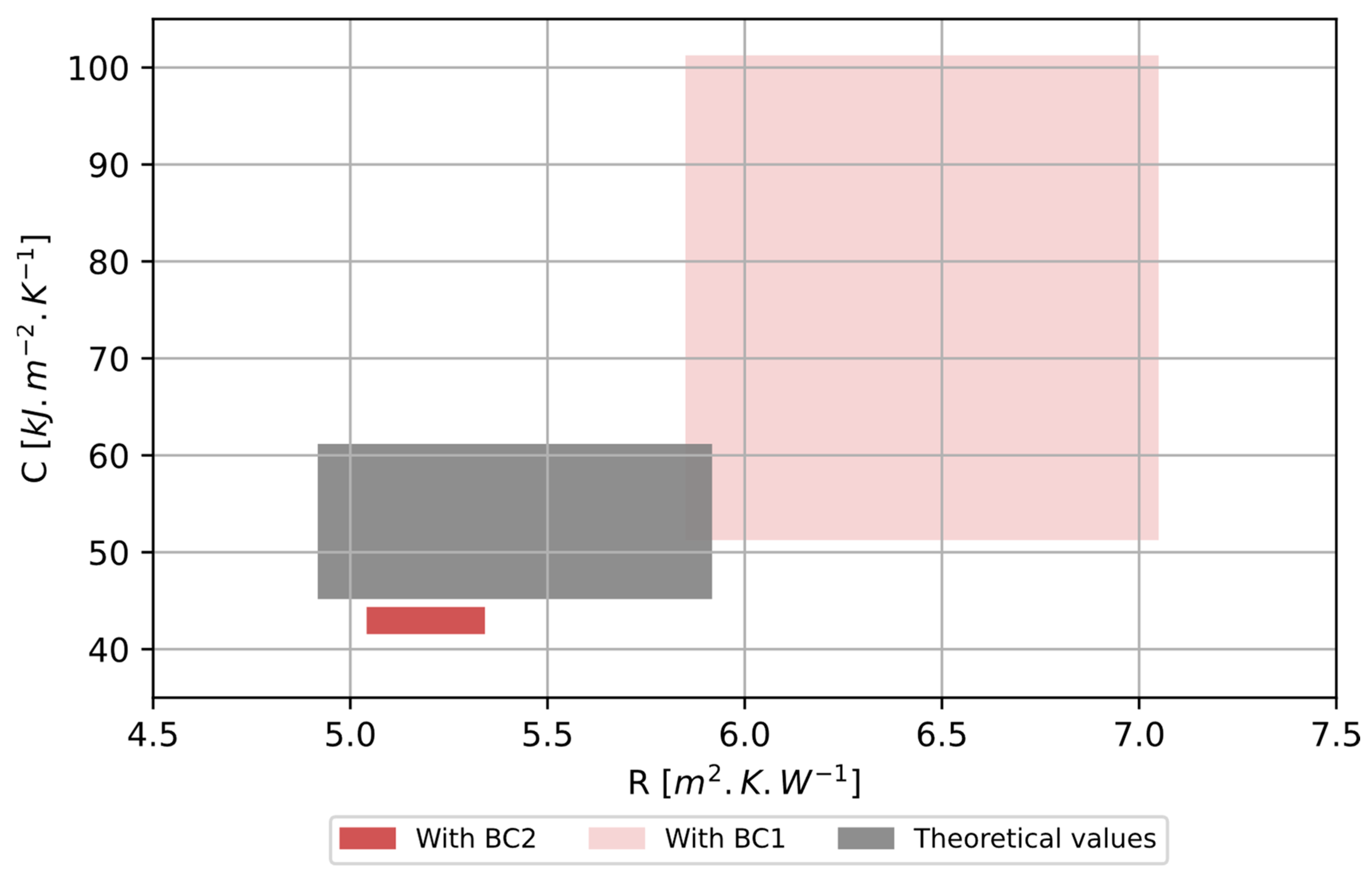
5.2. Application to Measured Experimental Data
6. Discussions
7. Conclusions
Author Contributions
Funding
Data Availability Statement
Acknowledgments
Conflicts of Interest
Nomenclature
| c | Specific heat capacity, J.kg−1.K−1 | Q | Heat flux density, W.m−2 |
| C | Total thermal mass, J.m−2.K−1 | R | Thermal resistance, m2.K.W−1 |
| d | Wind direction, ° | S | Sensor |
| e | Thickness of a layer, m | t | Time, s |
| h | Heat transfer coefficient, W.m−2.K−1 | T | Temperature, °C or K |
| L | Thickness of wall, m | v | Velocity, m.s−1 |
| MAD | Mean absolute deviation, °C | x | Space variable, m |
| Greek symbols | |||
| α | Absorptivity, - | λ | Thermal conductivity, W.m−1.K−1 |
| β | List of parameters to be estimated | ρ | Density, kg.m−3 |
| ε | Emissivity, - | σ | Stefan-Boltzmann constant, W.m−2.K−4 |
| Index and Exponent | |||
| →| | Received by device | PUR | Polyurethane |
| b | Brightness | pyrgeo | Pyrgeometer |
| conv | Convection | out | Outdoor |
| in | Indoor | S | Surface |
| LW | Longwave radiation | SW | Shortwave radiation |
| pl | Plywood | ||
References
- Meiss, A.; Feijó-Muñoz, J. The energy impact of infiltration: A study on buildings located in north central Spain. Energy Effic. 2015, 8, 51–64. [Google Scholar] [CrossRef]
- Eleftheriadis, G.; Hamdy, M. Impact of building envelope and mechanical component degradation on the whole building performance: A review paper. Energy Procedia 2017, 132, 321–326. [Google Scholar] [CrossRef]
- Asan, H.; Sancaktar, Y. Effects of Wall’s thermophysical properties on time lag and decrement factor. Energy Build. 1998, 28, 159–166. [Google Scholar] [CrossRef]
- NF EN 12939; Thermal Performance of Building Materials and products—Determination of Thermal Resistance by Means of Guarded Hot Plate and Heat Flow Meter Methods—Thick Products of High and Medium Thermal Resistance. British Standards Institution: London, UK, 2000.
- NF EN 12667; Thermal Performance of Building Materials and Products—Determination of Thermal Resistance by Means of Guarded Hot Plate and Heat Flow Meter Methods—Products of High and Medium Thermal Resistance. British Standards Institution: London, UK, 2001.
- Bienvenido-Huertas, D.; Moyano, J.; Marín, D.; Fresco-Contreras, R. Review of in situ methods for assessing the thermal transmittance of walls. Renew. Sustain. Energy Rev. 2019, 102, 356–371. [Google Scholar] [CrossRef]
- ISO 9869-1; Thermal Insulation—Building Elements—In-Situ Measurement of Thermal Resistance and Thermal Transmittance—Part 1: Heat Flow Meter Method. International Organization for Standardization: Geneva, Switzerland, 2014.
- Peng, C.; Wu, Z. In situ measuring and evaluating the thermal resistance of building construction. Energy Build. 2008, 40, 2076–2082. [Google Scholar] [CrossRef]
- Teni, M.; Krstić, H.; Kosiński, P. Review and comparison of current experimental approaches for in-situ measurements of building walls thermal transmittance. Energy Build. 2019, 203, 109417. [Google Scholar] [CrossRef]
- Beck, J.V.; Blackwell, B.; Clair, C.R.S. Inverse Heat Conduction: Ill-Posed Problems; Wiley: Hoboken, NJ, USA, 1985. [Google Scholar]
- Beck, J.V.; Arnold, K.J. Parameter Estimation in Engineering and Science; Wiley: Hoboken, NJ, USA, 1977. [Google Scholar]
- Orlande, H.R.; Fudym, O.; Maillet, D.; Cotta, R.M. Thermal Measurements and Inverse Techniques; CRC Press: Boca Raton, FL, USA, 2011. [Google Scholar] [CrossRef]
- Defer, D.; Shen, J.; Lassue, S.; Duthoit, B. Non-destructive testing of a building wall by studying natural thermal signals. Energy Build. 2002, 34, 63–69. [Google Scholar] [CrossRef]
- Sassine, E. A practical method for in-situ thermal characterization of walls. Case Stud. Therm. Eng. 2016, 8, 84–93. [Google Scholar] [CrossRef]
- Rasooli, A.; Itard, L.; Ferreira, C.I. A response factor-based method for the rapid in-situ determination of wall’s thermal resistance in existing buildings. Energy Build. 2016, 119, 51–61. [Google Scholar] [CrossRef]
- Rasooli, A.; Itard, L. In-situ rapid determination of walls’ thermal conductivity, volumetric heat capacity, and thermal resistance, using response factors. Appl. Energy 2019, 253, 113539. [Google Scholar] [CrossRef]
- Gutschker, O. Parameter identification with the software package LORD. Build. Environ. 2008, 43, 163–169. [Google Scholar] [CrossRef]
- Baker, P.; van Dijk, H. PASLINK and dynamic outdoor testing of building components. Build. Environ. 2008, 43, 143–151. [Google Scholar] [CrossRef]
- Loussouarn, T.; Maillet, D.; Remy, B.; Schick, V.; Dan, D. Indirect measurement of temperature inside a furnace, ARX model identification. J. Phys. Conf. Ser. 2018, 1047, 012006. [Google Scholar] [CrossRef]
- Jiménez, M.; Heras, M. Application of multi-output ARX models for estimation of the U and g values of building components in outdoor testing. Sol. Energy 2005, 79, 302–310. [Google Scholar] [CrossRef]
- Naveros, I.; Ghiaus, C.; Ruíz, D.; Castaño, S. Physical parameters identification of walls using ARX models obtained by deduction. Energy Build. 2015, 108, 317–329. [Google Scholar] [CrossRef]
- Limam, K.; Bouache, T.; Ginestet, S.; Popescu, L.O. Numerical and experimental identification of simplified building walls using the reflective Newton method. J. Build. Phys. 2018, 41, 321–338. [Google Scholar] [CrossRef]
- Naveros, I.; Bacher, P.; Ruiz, D.; Jiménez, M.; Madsen, H. Setting up and validating a complex model for a simple homogeneous wall. Energy Build. 2014, 70, 303–317. [Google Scholar] [CrossRef]
- Berger, J.; Orlande, H.R.; Mendes, N.; Guernouti, S. Bayesian inference for estimating thermal properties of a historic building wall. Build. Environ. 2016, 106, 327–339. [Google Scholar] [CrossRef]
- Biddulph, P.; Gori, V.; Elwell, C.A.; Scott, C.; Rye, C.; Lowe, R.; Oreszczyn, T. Inferring the thermal resistance and effective thermal mass of a wall using frequent temperature and heat flux measurements. Energy Build. 2014, 78, 10–16. [Google Scholar] [CrossRef]
- Rouchier, S.; Woloszyn, M.; Kedowide, Y.; Béjat, T. Identification of the hygrothermal properties of a building envelope material by the covariance matrix adaptation evolution strategy. J. Build. Perform. Simul. 2015, 9, 101–114. [Google Scholar] [CrossRef]
- Wang, S.; Xu, X. Parameter estimation of internal thermal mass of building dynamic models using genetic algorithm. Energy Convers. Manag. 2006, 47, 1927–1941. [Google Scholar] [CrossRef]
- Chaffar, K.; Chauchois, A.; Defer, D.; Zalewski, L. Thermal characterization of homogeneous walls using inverse method. Energy Build. 2014, 78, 248–255. [Google Scholar] [CrossRef]
- Dall‘O’, G.; Sarto, L.; Panza, A. Infrared Screening of Residential Buildings for Energy Audit Purposes: Results of a Field Test. Energies 2013, 6, 3859–3878. [Google Scholar] [CrossRef]
- de Rubeis, T.; Evangelisti, L.; Guattari, C.; De Berardinis, P.; Asdrubali, F.; Ambrosini, D. On the Influence of Environmental Boundary Conditions on Surface Thermal Resistance of Walls: Experimental Evaluation through a Guarded Hot Box. Case Stud. Therm. Eng. 2022, 34, 101915. [Google Scholar] [CrossRef]
- Evangelisti, L.; Guattari, C.; Gori, P.; Vollaro, R.d.L.; Asdrubali, F. Experimental Investigation of the Influence of Convective and Radiative Heat Transfers on Thermal Transmittance Measurements. Int. Commun. Heat Mass Transf. 2016, 78, 214–223. [Google Scholar] [CrossRef]
- François, A.; Ibos, L.; Feuillet, V.; Meulemans, J. Novel in Situ Measurement Methods of the Total Heat Transfer Coefficient on Building Walls. Energy Build. 2020, 219, 110004. [Google Scholar] [CrossRef]
- Derbal, R.; Defer, D.; Chauchois, A.; Antczak, E. A simple method for building materials thermophysical properties estimation. Constr. Build. Mater. 2014, 63, 197–205. [Google Scholar] [CrossRef]
- Spitz, C.; Mora, L.; Wurtz, E.; Jay, A. Practical application of uncertainty analysis and sensitivity analysis on an experimental house. Energy Build. 2012, 55, 459–470. [Google Scholar] [CrossRef]
- EN ISO 6946; Building Components and Building Elements—Thermal Resistance and Thermal Transmittance—Calculation Method. International Organization for Standardization: Geneva, Switzerland, 2017.
- Macdonald, I.A. Quantifying the Effects of Uncertainty in Building Simulation. Ph.D. Thesis, University of Strathclyde, Glasgow, UK, 2002. [Google Scholar]
- CSTB. Règles Th-bat—Fascicule Matériaux (French Building Regulation). France, 2017. Available online: https://rt-re-batiment.developpement-durable.gouv.fr/IMG/pdf/2-fascicule_materiaux.pdf (accessed on 14 November 2024).
- Ross, R.J. Wood Handbook: Wood as an Engineering Material; U.S. Dept. of Agriculture, Forest Service, Forest Products Laboratory: Madison, WI, USA, 2010; Volume 190. [Google Scholar]
- Cattarin, G.; Causone, F.; Kindinis, A.; Pagliano, L. Outdoor test cells for building envelope experimental characterization—A literature review. Renew. Sustain. Energy Rev. 2016, 54, 606–625. [Google Scholar] [CrossRef]
- Spampinato, L.; Calvari, S.; Oppenheimer, C.; Boschi, E. Volcano surveillance using infrared cameras. Earth-Sci. Rev. 2011, 106, 63–91. [Google Scholar] [CrossRef]
- Orme, M. Applicable Models for Air Infiltration and Ventilation Calculations; AIVC: Vancouver, BC, Canada, 1999. [Google Scholar]
- Madsen, H.; Bacher, P.; Bauwens, G.; Deconinck, A.H.; Reynders, G.; Roels, S.; Himpe, E.; Lethé, G. Thermal Performance Characterization using Time Series Data. In IEA EBC Annex 58 Guidelines; International Energy Agency: Paris, France, 2015. [Google Scholar]
- Maillet, D.; André, S.; Batsale, J.-C.; Degiovanni, A.; Moyne, C. Thermal Quadrupoles: Solving the Heat Equation Through Integral Transforms; Wiley: Hoboken, NJ, USA, 2000. [Google Scholar]
- Brun, A. Amélioration du confort d’été dans des bâtiments à ossature par ventilation de l’enveloppe et stockage thermique. Ph.D. Thesis, Université de Grenoble, Saint-Martin-d’Hères, France, 2011. [Google Scholar]
- Khalifa, A.; Marshall, R. Validation of heat transfer coefficients on interior building surfaces using a real-sized indoor test cell. Int. J. Heat Mass Transf. 1990, 33, 2219–2236. [Google Scholar] [CrossRef]
- Peeters, L.; Beausoleil-Morrison, I.; Novoselac, A. Internal convective heat transfer modeling: Critical review and discussion of experimentally derived correlations. Energy Build. 2011, 43, 2227–2239. [Google Scholar] [CrossRef]
- Awbi, H.; Hatton, A. Natural convection from heated room surfaces. Energy Build. 1999, 30, 233–244. [Google Scholar] [CrossRef]
- Defraeye, T.; Blocken, B.; Carmeliet, J. Convective heat transfer coefficients for exterior building surfaces: Existing correlations and CFD modelling. Energy Convers. Manag. 2011, 52, 512–522. [Google Scholar] [CrossRef]
- ASHRAE Task Group. Procedure for Determining Heating and Cooling Loads for Computerizing Energy Calculations: Algorithms for Building Heat Transfer Subroutines; American Society of Heating, Refrigerating and Air-Conditioning Engineers: Peachtree Corners, GA, USA, 1976. [Google Scholar]
- Sharples, S. Full-scale measurements of convective energy losses from exterior building surfaces. Build. Environ. 1984, 19, 31–39. [Google Scholar] [CrossRef]
- Liu, Y.; Harris, D. Full-scale measurements of convective coefficient on external surface of a low-rise building in sheltered conditions. Build. Environ. 2007, 42, 2718–2736. [Google Scholar] [CrossRef]
- COMSOL. COMSOL Multiphysics 5.5 Reference Manual. 2019. Available online: https://doc.comsol.com/5.5/doc/com.comsol.help.comsol/COMSOL_ReferenceManual.pdf (accessed on 14 November 2024).
- Tsilingiris, P. Parametric space distribution effects of wall heat capacity and thermal resistance on the dynamic thermal behavior of walls and structures. Energy Build. 2006, 38, 1200–1211. [Google Scholar] [CrossRef]
- Petit, D.; Maillet, D. Techniques inverses et estimation de paramètres. Partie 1. Tech. Ing. Phys. Stat. Mathématique 2008, 42619210, 1–18. [Google Scholar]
- Nelder, J.A.; Mead, R. A Simplex Method for Function Minimization. Comput. J. 1965, 7, 308–313. [Google Scholar] [CrossRef]
- Remy, B.; Degiovanni, A. Parameters estimation and measurement of thermophysical properties of liquids. Int. J. Heat Mass Transf. 2005, 48, 4103–4120. [Google Scholar] [CrossRef]


| Physical Variable | Sensor | Acquisition | Accuracy |
|---|---|---|---|
| Indoor air temperature | PT100 1/5 B DIN, 4 wires (TCSA) | KEYSIGHT 34980A | ±0.15 °C * |
| Surface temperature | PT100 1/3 B DIN, 4 wires (TCSA) | ||
| Interface temperature | |||
| Outdoor air temperature | PT100 (VAISALA HMP1550) | COMPACT DAQ NI 9188 | |
| Shortwave radiation | SMP21 (KIPP AND ZONEN) | RS 485—Modbus | ±3 W.m−2 ** |
| Brightness temperature | SGR4 (KIPP AND ZONEN) | ±0.7 °C ** | |
| Wind velocity | WINCAP Ultrasonic WMT701 (VAISALA) | ±0.1 m.s−1 ** | |
| Wind direction | ±2° ** |
| λpl | λPUR | (ρ.c)pl | (ρ.c)PUR | |
|---|---|---|---|---|
| λpl | 1 | −0.24 | 0.24 | −0.03 |
| λPUR | 1 | −0.05 | 0.16 | |
| (ρ.c)pl | 1 | −0.95 | ||
| (ρ.c)PUR | 1 |
| Parameter | RC | COMSOL | ||
|---|---|---|---|---|
| Modelling | Space | Number | 21 nodes | 28 elements |
| Time | Boundary conditions | 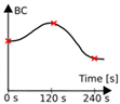 |  | |
| Time step | 120 s | 10 s | ||
| Identification results | BC1 | R | ±10% | |
| C | ±47% | |||
BC2 | R | ±3% | ||
| C | ±3% | |||
Disclaimer/Publisher’s Note: The statements, opinions and data contained in all publications are solely those of the individual author(s) and contributor(s) and not of MDPI and/or the editor(s). MDPI and/or the editor(s) disclaim responsibility for any injury to people or property resulting from any ideas, methods, instructions or products referred to in the content. |
© 2024 by the authors. Licensee MDPI, Basel, Switzerland. This article is an open access article distributed under the terms and conditions of the Creative Commons Attribution (CC BY) license (https://creativecommons.org/licenses/by/4.0/).
Share and Cite
Rendu, M.; Le Dréau, J.; Salagnac, P.; Doya, M. Influence of Boundary Conditions on the Estimation of Thermal Properties in Insulated Building Walls. Buildings 2024, 14, 3706. https://doi.org/10.3390/buildings14123706
Rendu M, Le Dréau J, Salagnac P, Doya M. Influence of Boundary Conditions on the Estimation of Thermal Properties in Insulated Building Walls. Buildings. 2024; 14(12):3706. https://doi.org/10.3390/buildings14123706
Chicago/Turabian StyleRendu, Manon, Jérôme Le Dréau, Patrick Salagnac, and Maxime Doya. 2024. "Influence of Boundary Conditions on the Estimation of Thermal Properties in Insulated Building Walls" Buildings 14, no. 12: 3706. https://doi.org/10.3390/buildings14123706
APA StyleRendu, M., Le Dréau, J., Salagnac, P., & Doya, M. (2024). Influence of Boundary Conditions on the Estimation of Thermal Properties in Insulated Building Walls. Buildings, 14(12), 3706. https://doi.org/10.3390/buildings14123706