Abstract
Productive facades, consisting of photovoltaic shading and vertical farming systems, have been proposed as a means to improve the thermal and visual status of residential buildings while also maintaining energy performance and providing vegetables. However, how to quickly and accurately predict electricity and vegetable output during the numerous influencing architectural and environmental factors is one of the key issues in the early stages of design, and few studies have investigated the impact of such structures on both indoor environmental qualities and production performance. In this paper, we present a novel prediction method that uses experimental data to train and test an artificial neural network (ANN). The results indicated that using the Bipolar Sigmoid activation function to process the experimental data input to the artificial neuron network gives more accurate predicted results both in the yield of photovoltaic shading and vertical farming systems. In addition, this prediction method was applied to a typical high-rise residential building in Singapore to assess the self-sufficiency potential of high-rise residential buildings integrated with productive facades. The results indicated that the upper part of the building can meet 20.0–23.1% of the annual household electricity demand of a family of four in a four-room residential unit in Singapore and almost the entire year’s vegetable demand, while the middle part can meet 18.4–21.2% and 89.1%, respectively. The results demonstrated the importance of a productive facade in reducing energy demand, enhancing food security, and improving indoor visual and thermal comfort.
1. Introduction
More than half of the world’s population is concentrated in cities that occupy 2% of the Earth’s surface [1]. Buildings in cities represent 36% of the global final energy consumption [2]. This energy demand is always increasing, and the lack of clean energy resources to cover it is a major challenge in reducing the urban carbon footprint. Moreover, the energy consumption of the residential sector is more than three times that of the non-residential sector [3]. As people’s demand for environmental comfort grows, the proportion of “air-conditioned” buildings continues to rise [4]. Reducing the energy consumption of residential buildings and improving the comfort of the indoor environment are important parts of solving the urban energy crisis and improving the quality of the human settlement environment. In addition, the urban-rural gap and globalization have significantly increased food mileage [5]; however, it is still hugely challenging to fully obtain healthy and affordable food in many cities and regions [6]. At present, vertical farming has been adopted to address the limitations of traditional agriculture, the shrinking area of arable land, and increasing food demand [7,8]. However, there is still a lack of research on the potential crop yields of building facades [9,10].
To address environmental and energy problems, a variety of facade design methods and concepts have been proposed in the field of architecture aimed at improving indoor environmental quality [11], significantly reducing building energy consumption [12], and generating a positive impact on local renewable resources, buildings, and human resource consumption [13]. In recent years, the concept of productive facade systems has been introduced by Tablada et al. (2018), in which PV shading devices and vertical farming systems are integrated into building facades. Taking into account the balance between BIPV and BIA, PV shading is usually located in the upper part of the window, while vertical farming is located in the lower part, in order to adapt to the respective system requirements and ensure the accessibility of the indoor view [14]. In addition, the integrated PV module design and modular planting slots are used to ensure the aesthetic effect of the building façade [15].
Simulations and experimental results have shown that this integration can help achieve sustainability goals at urban and building scales by alleviating urban energy shortages and improving urban food security while improving indoor environmental quality [9,16].
However, predicting the yields of PV shading and vertical farming systems is complex. Previous studies were based on empirical formulas or simulation tools; however, more recent studies have shown that the calculated results of these methods and tools often have non-negligible errors compared to the actual results [17]. This is because these two systems are affected by multiple environmental factors, such as solar radiation, ambient temperature, shadow, soil fertility, precipitation, and wind speed.
Theoretically, the solar radiation received by a PV module gets converted into electricity at a certain conversion rate; however, under actual conditions, this yield is reduced by both the temperature and the shadow of the PV cell. Regarding prediction of module temperature, Zhen and Nobre et al. (2013) reported that, in Singapore, the k value (Ross coefficient) of PV modules can reach as much as twice that of the same type of PV module but installed in a different environment [18]. PV fabricators provide the PV temperature coefficient of power, which governs how strongly the conversion efficiency depends on temperature. However, after a module reaches a certain temperature, the coefficient has a large error compared to the actual situation, which causes the PV temperature coefficient of power to not meet the design accuracy requirements. Regarding shadows, they not only cause electrical mismatch losses in different parts of a PV module but also overheat the panel [19].
In terms of vegetable yield, it is difficult to obtain accurate yield data using formulas or simulation methods due to several climatic variables and planting methods. Previous studies have often estimated vegetable yields based on the planting area and incident radiation, but this rough calculation method ignores other climatic variables and external factors, such as DLI, composts, and crop rotation [20].
As problems in the building field become more complicated, the above-mentioned common methods gradually lose their advantages in terms of time, cost, and reliability. Simultaneously, machine learning methods represented by ANNs have gradually become crucial for seeking architectural solutions [21]. ANNs can improve the accuracy of prediction results by using more complex functional relationships for modeling. In recent years, it has been used in building performance prediction [22,23] and has proven to be highly efficient for rapid assessment of building performance [24,25]. In particular, PV power yield prediction models have been proposed based on ANNs [26,27]. A multilayer perceptron (MLP)-based ANN architecture has been used to predict a PV plant power yield using three input elements [28]. An ANN for PV panels has been developed, which uses the root mean square error (RMSE) method to evaluate the prediction quality of the ANN [29]. Several commonly used input elements, such as global horizontal irradiance (GHI), azimuth and altitude angles, air temperature, module tilt angle and surface temperature, and date [30,31,32], are mainly aimed at predicting the yield under environmental conditions such as PV power stations and rooftop PV. However, there is insufficient research on the prediction of PV yield under building facade installation conditions, especially with regard to solar PV shading. This problem becomes more apparent with the promotion of integrated photovoltaics.
Regarding the prediction of farming yield, Abrougui et al. (2019) used an ANN to predict organic potato yield [33]. Their ANN had greater potential to estimate yield compared to a multiple linear regression model. Saad et al. (2009) proposed an ANN to predict rice yield [34], and Pantazi et al. (2016) applied an ANN to predict wheat yield using soil and remote sensing vegetation indices as input parameters [35]. The input elements typically include tillage systems and soil properties [33]. Although ANNs are widely used for predicting farming yield, research on vertical farming is still lacking.
Several tools, such as MATLAB and Grasshopper, have a toolbox for ANNs. For Grasshopper, four known plugins adopt ANN algorithms: Dodo, Crow, Owl, and Lunchbox [36,37]. The 3D modeling software Rhinoceros 6.0 and its Grasshopper plug-in have been used to control geometric parameters and analyze indoor environmental performance [38].
This study first compared the predictive modeling methods using ANN with different activation functions, proposed a relatively fast and reliable method for assisting productive facade design, and then explored the application of ANN predictions in practice to evaluate productive facade yield performance. The overall prediction process, shadow analysis, and solar radiation analysis were performed using the Grasshopper plug-in for the Rhinoceros platform. In addition, the indoor daylight and thermal environment of a residential unit were compared using this platform [38,39].
2. Materials and Methods
To obtain reliable PV electricity yield and vertical farming vegetable yield data, this study combined an ANN trained and tested by experimental data (given in Appendix A) from the NUS-CDL Tropical Technologies Laboratory (T2 Lab) of the National University of Singapore (NUS) [27,40]. The experimental data included the PV shading electricity yield (monocrystalline silicon, type: assembled by the Solar Energy Research Institute of Singapore/CIGS thin film, type: Solar Frontier SFL85-D) and vertical farming vegetable yield data (lettuce planting). Details of the T2 Lab PV shading system are shown in Table 1 and Figure 1, and the performance indicators of the T2 Lab envelope are shown in Table 2.

Table 1.
Key parameters of monocrystalline silicon and CIGS thin film used in the T2 Lab.
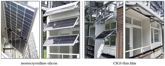
Figure 1.
Details of the T2 Lab PV shading system.
Table 2.
The performance indicators of the T2 Lab envelope.
The proposed ANN was trained using experimental data to obtain a predictive model that correlated the environmental and yield elements. Figure 2 depicts two predictive models: Predictive model 1 (environmental and PV shading electricity yield elements) and Predictive model 2 (environmental and vertical farming vegetable yield elements). Through predictive modeling, this paper presents the yield on the southern productive facade of a typical public housing building (point block) in Singapore and analyzes indoor thermal and visual comfort.
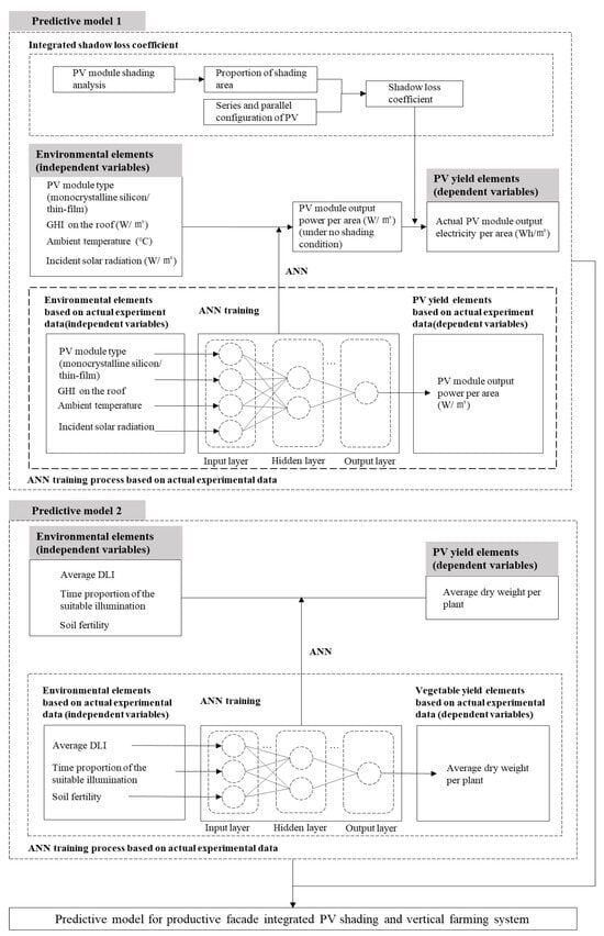
Figure 2.
Framework of the two predictive ANNs.
The experimental data were from April 2019 to May 2019 (for PV shading, Figure 3) and from December 2018 to June 2019 (for vertical farming, Figure 4). The recorded data included: ① GHI (type: SPN1-A1815, W/m2); ② ambient temperature (type: RM Young 92000, °C); ③ wind speed (type: RM Young 05103, m/s); ④ PV module’s temperature (type: RTD Pt 100, °C); ⑤ incident solar radiation (type: IMT Si-420TC, W/m2); ⑥ output electricity recorded by a maximum power point tracking controller (type: BlueSolar charge controller MPPT, Wh/m2); ⑦ vertical farming data including the photosynthetic photon flux density (PPFD, type: Quantum PAR Meter); ⑧ average dry weight of each plant in each planting cycle. The data collection frequency is once per minute (①–⑦).
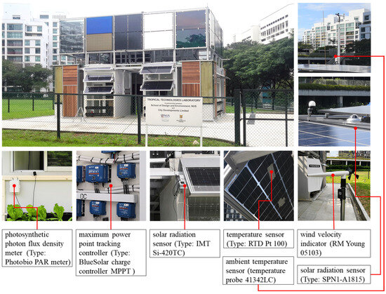
Figure 3.
NUS T2 Lab and testing sensor.
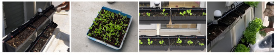
Figure 4.
Planting, cultivation, and picking process of lettuce in T2 Lab.
In this study, two solutions were adopted to reduce the unreliable training data caused by the impact of environmental shadows on the PV module, which causes the hotspot effect. First, the uppermost PV module was selected to avoid shading between the PV modules. For example, there were nine monocrystalline silicon PV modules (assembled by the Solar Energy Research Institute of Singapore) facing east and west in the laboratory, and only three of the uppermost modules (module tilt angle: 40°) were selected. Second, we prevented the laboratory from blocking the PV modules. The CIGS thin-film PV modules (Type: Solar Frontier SFL85-D) in the north and south directions were all single-layer (module tilt angle: 20°), but the sun was located north of Singapore during the collection of the experimental data; therefore, only the north PV module was selected. Furthermore, the east, west, and north modules intercepted the experimental data from 6 a.m.–12 a.m. (6 h), 12 a.m.–6 p.m. (6 h), and 6 a.m.–6 p.m. (12 h). In this study, the experimental output power data of each PV module was converted into output electricity per unit area (Wh/m2). The predictive ANN was only applied to single-layer monocrystalline silicon and single-layer thin-film PV modules, owing to the aforementioned deliberate selection of experimental data. In addition, the electricity yield of PV shading was predicted for a variety of module angles because the predictive ANN was trained with substantial data that covered a significantly broad range.
The predictive model aimed to connect the environmental elements (independent variables) with the yield elements (dependent variables). This type of problem is mainly addressed in machine learning through supervised learning in training methods, specifically through an ANN in regression tasks. In this study, the back-propagation algorithm was used to train an ANN with an MLP structure [30]. Two commonly used activation functions (the Bipolar Sigmoid and SoftPlus functions) in the back-propagation algorithm were compared to select the optimal function, and the multiple linear regression model of machine learning was chosen as a reference. In addition, ANN evaluations usually include training and testing errors. Training error expresses an ANNs quality of fit to the training data. If the training error is too large, the ANN has insufficient knowledge of the training data characteristics. Otherwise, the ANN has overlearned the characteristics of the training data if the training error is too small. Therefore, maintaining appropriate training errors is crucial for evaluating the quality of an ANN. In contrast to the training error, the test error characterizes the generalization ability of an ANN. In practical applications, the test error must be as small as possible.
The predictive models were calculated using the Grasshopper plug-in Dodo [23,41] and Rhinoceros 3D software [42]. Dodo was created by Lorenzo Greco and features an extensive set of components for ANNs [23]. Rhinoceros and Grasshopper provide a familiar operating platform for designers to establish predictive models and analyze the environmental performance of residential units.
2.1. Predictive Model 1: Environmental and PV Shading Electricity Yield Elements
Based on an ANN combined with the shadow loss coefficient, a predictive model was developed for environmental and PV shading electricity yield elements. The model contains two steps: the first establishes the ANN, and the second couples shadow influences. The second was training the ANN using the experimental data from the T2 Lab from April to May 2019. The input variables of the ANN were initially set to five environmental elements (independent variables: GHI on the roof, ambient temperature, wind speed, PV module temperature, and PV module incident solar radiation), and the output variable was only the PV shading electricity yield element (dependent variable: PV module output electricity per unit area (Wh/m2). In the second step, according to the mechanism of the PV module being affected by the shadow and the common methods to reduce shadow influence, the shadow influence was converted into the shadow loss coefficient, which was then coupled with the ANN model from the first step.
2.1.1. Correlation Analysis
Using a monocrystalline silicon PV module as an example, the Pearson correlation coefficient was used to analyze the correlation between the five environmental elements (independent variables) and one PV electricity yield element (dependent variable). We analyzed the experimental data through SPSS 22.0 from April to May 2019 containing 65,880 sets (3 modules × 61 d × 6 h × 60 min) from three monocrystalline silicon PV modules placed in the east and west orientations of the T2 Lab. The results are listed in Table 3. The correlation coefficients were all greater than 0.4 [43] except “wind speed”, indicating a moderate or strong positive correlation between the independent and dependent variables. However, the PV module temperature and wind speed were excluded from the variable types after considering their time cost, feasibility, and relatively low correlation coefficients for the five independent variables. Finally, each set of experimental data contained three types of environmental elements (independent variables: GHI on the roof, ambient temperature, and PV module incident solar radiation) and one type of PV shading electricity yield element (dependent variable: PV module output electricity per unit area).
Table 3.
Correlation analysis between environmental and PV shading electricity yield elements.
2.1.2. First Step: Building the ANN
ANN Training
The Latin cube sampling method was used to divide the actual experimental data into training (70%) and validation (30%) data [44]. Each set of training data and validation data contained three independent variables: GHI on the roof, ambient temperature, PV module incident solar radiation, and one dependent variable: PV module output electricity per unit area. The categories and contents of each set of data are listed in Appendix A Table A3 and Table A4.
The root mean square error (RMSE) and mean absolute error (MAE) were used to analyze the training and test errors of different ANNs [28,45]. The other ANN parameter settings are listed in Table 4.
Table 4.
ANN parameter settings for predictive model 1.
① The experimental data of the monocrystalline silicon PV module were recorded by three PV modules in the east and west directions of the T2 Lab of NUS from April to May 2019 for a total of 61 days. There were 65,880 sets of data (3 modules × 61 d × 6 h × 60 min), of which 46,116 and 19,764 sets were used as training and test data, respectively. (Due to space limitations, only part of the data are shown in Appendix A Table A3).
② The source of the experimental data for thin-film PV modules was the same as that for monocrystalline silicon PV modules. The difference was that one thin-film cell was facing north, and there were 43,920 sets of data (1 module × 61 d × 12 h × 60 min), of which 30,744 and 13,176 sets were used as training and test data, respectively. (Due to space limitations, only part of the data are shown in Appendix A Table A4).
ANN Evaluation
The RMSE is the square root of the average of the sum of squares of each data deviation from the true value. Its expression is
where is the actual experimental value, and is the predicted value of the ANN.
The MAE is the average value of the absolute error, which can better reflect the true situation of the predicted value error. It is expressed as
- (1)
- Evaluation of the ANN for monocrystalline silicon PV modules.
As shown in Figure 5 and Table 5, the training and test errors of the three models (two ANNs and one multiple linear regression model) were relatively suitable. Therefore, there were no overfitting or underfitting situations in the model. Further analysis showed that the overall prediction quality was higher for the ANN than that for multiple linear regression. In terms of the activation function for the ANN, SoftPlus was more effective than Bipolar Sigmoid when considering RMSE; however, for MAE, the former was less effective than the latter.
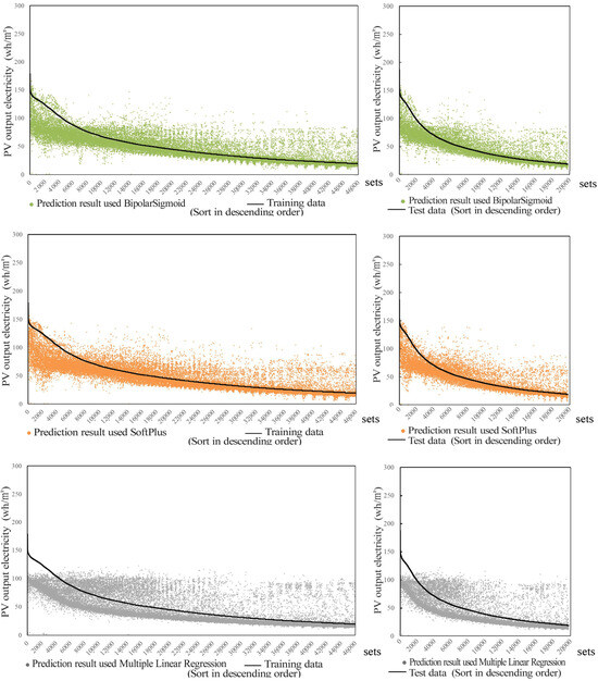
Figure 5.
Visualization of prediction results of different methods for monocrystalline silicon PV modules.
Table 5.
Analysis of training and test errors of different methods for monocrystalline silicon PV modules.
Compared to MAEs, RMSEs give more weight to the abnormal points in the data. Therefore, the abnormal points in the data cause the RMSE to shift towards the abnormal points at the expense of other data points, thereby reducing the overall prediction quality of an ANN. Specifically, for MAE, the training and test errors of the SoftPlus activation function were 5.8% and 4.4% higher than those of the Bipolar Sigmoid function, respectively. For RMSE, the training and test errors of SoftPlus were 6.1% and 6.0% lower than those of the Bipolar Sigmoid function, respectively. Therefore, the prediction results of the ANN using the SoftPlus activation function had fewer abnormal points than those using the Bipolar Sigmoid, which is crucial. We also showed that the ANN using the SoftPlus activation function had a better prediction quality.
Figure 6 shows the comparison between the predicted and experimental results for evaluation. Considering fitting, the fit for the ANN model using the SoftPlus activation function was highest (R2 = 0.66 for Bipolar Sigmoid; R2 = 0.69 for SoftPlus; and R2 = 0.60 for multiple linear regression) [46]. Finally, the ANN with the SoftPlus function was selected as the ANN module for the monocrystalline silicon PV.
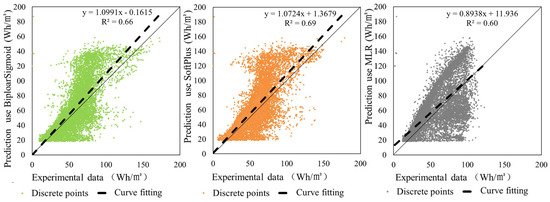
Figure 6.
Comparison of predicted and experimental results in terms of different methods for monocrystalline silicon PV modules.
- (2)
- Evaluation of the ANN for thin-film PV module
Similar to the evaluation of the monocrystalline silicon PV module, Figure 7 and Table 6 show that the training and test errors of the three models (two ANNs and one multiple linear regression model) were relatively suitable for the thin-film PV module. There was also no overfitting or underfitting of the model. Further analysis showed that the ANN had smaller errors and clear advantages over multiple linear regression. In addition, the MAE and RMSE values of the ANN using the Bipolar Sigmoid activation function were smaller than those for the SoftPlus activation function. Moreover, Figure 8 shows that the ANN prediction results with the Bipolar Sigmoid activation function fit the experimental data better than the other two (R2 = 0.88 for Bipolar Sigmoid; R2 = 0.78 for SoftPlus; and R2 = 0.52 for multiple linear regression) [46]. Therefore, the ANN with the Bipolar Sigmoid activation function was selected as the ANN for the thin-film PV modules.
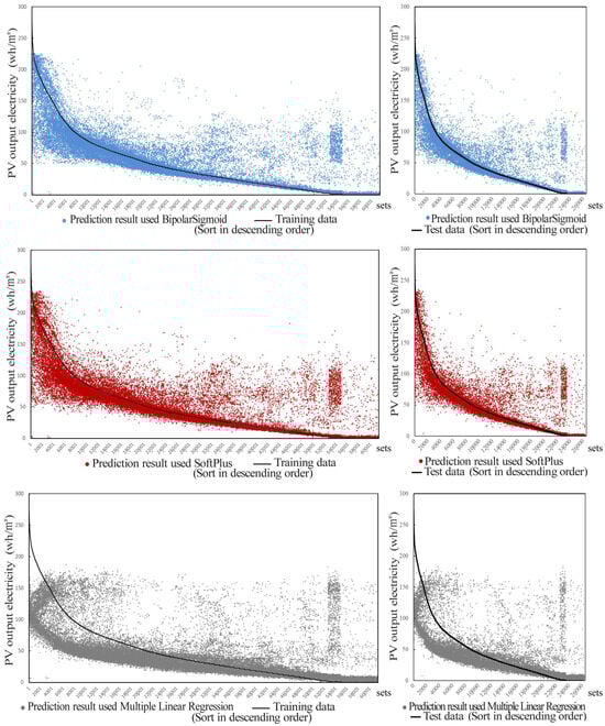
Figure 7.
Visualization of prediction results from different methods for thin-film PV modules.
Table 6.
Analysis of training and test errors from different methods for thin-film PV modules.
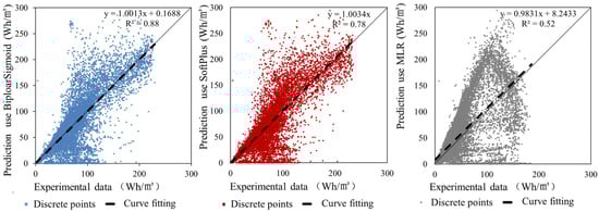
Figure 8.
Comparison of prediction and experimental results from different methods for thin-film PV modules.
Establishment of the ANN
According to the model evaluation, the ANN with the SoftPlus activation and Bipolar Sigmoid activation functions were selected as the prediction models for the yield of the monocrystalline silicon and thin-film PV modules, respectively. The specific information about the models is listed in Table 7.
Table 7.
The specific information in the ANN.
2.1.3. The Second Step: Integrated Shadow Loss Coefficient
Considering the different characteristics of the two types of PV modules (monocrystalline silicon and thin-film cells), as well as the calculation complexity and time cost, the shadow loss coefficient is defined as
where is the shadow loss coefficient, (based on Rhino 3D shadow analysis) is the area of the shaded part of the PV module, and is the area of the PV module.
2.2. Predictive Model 2—Environmental and Vertical Farming Vegetable Yield Elements
The experimental data were collected from six consecutive rounds of lettuce planting data (21 groups in total) during a half-year period from the T2 Lab of NUS [47] (Appendix A Table A1 and Table A2). Three factors were selected as the environmental elements (independent variables: average DLI of the planting cycle; time proportion of suitable illumination, which means the proportion of the total time that the PPFD received by the lettuce was in a suitable interval during the planting cycle; and soil fertility). Additionally, we selected the vertical farming vegetable yield element (dependent variable: average dry weight per plant). The experimental data were used to train the ANN and establish Predictive Model 2 (Appendix A Table A5).
2.2.1. Correlation Analysis
The Pearson correlation coefficient method was used to analyze the three environmental elements (independent variables) and one vertical farming vegetable yield element (dependent variable). Table 8 illustrates that the correlation coefficients between the environmental and vertical farming vegetable yield elements were all greater than 0.4 [43]; therefore, there is a moderate correlation, which can be used as training data to train the ANN.
Table 8.
Correlation analysis between the environmental and vertical farming yield elements.
2.2.2. Building the ANN
There are three steps in establishing the prediction model: training, evaluation, and establishing ANN.
ANN Training
The experimental data processing and model evaluation methods were identical to those used for the PV section. There were 21 sets of training data, and each set of data contained three types of environmental elements: ① average DLI during the planting cycle (mol/m2/d), ② time proportion of suitable illumination, and ③ soil fertility. In addition, there was one yield element for the vertical farming system, the average dry weight per plant (g). The mean ANN parameter settings are listed in Table 9.
Table 9.
ANN parameter settings for predictive model 2.
ANN Evaluation
Figure 9 and Table 10 show that the training and test errors of the three models were relatively suitable. The model training results were similar to those of the PV section. Further analysis showed that the overall prediction quality of the ANN was better than that of the multiple linear regression. Specifically, considering the MAE, the training error of the Bipolar Sigmoid activation function was 2.6% higher than that of SoftPlus, but the test error was 44.8% lower. For the RMSE, the training error of the Bipolar Sigmoid was 19% higher than that of SoftPlus, but the test error was 55.1% lower. To further evaluate the quality of the prediction models, the prediction results were compared to the experimental results (Figure 10), and it can be seen from the figure that the ANN prediction results using the Bipolar Sigmoid activation function fit the experimental data better than the other two (R2 = 0.63 for Bipolar Sigmoid; R2 = 0.61 for SoftPlus; and R2 = 0.47 for multiple linear regression [46] (The larger the R2-value is, the closer the curve fits to the diagonal, the better the model’s prediction results).
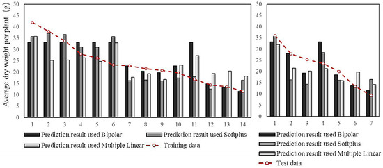
Figure 9.
Visualization of prediction results from different methods for vegetable farming yield.
Table 10.
Analysis of training and test errors from different methods for vertical farming yield.
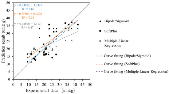
Figure 10.
Comparison of prediction results and experimental data from different methods for vertical farming yield.
Establishing ANN
According to the results of the model evaluation, the ANN with the Bipolar Sigmoid activation function was selected as the predictive model for the yield of vertical farming. The specific information about the model is listed in Table 11.
Table 11.
The specific information in the model.
2.3. Application of Predictive Models
As illustrated in Figure 11, the research objects were selected from the Arcadia community in Punggol, Singapore. Two residential units were selected in the HDB building 289D (18 floors): one on the high zone (15th floor as the representative floor) and the other on the middle zone (9th floor as the representative floor). The building is a typical contemporary block high-rise residential building [48]. Considering the layout of the surrounding area [49], it is one of seven high-rise residential buildings rotated 30° from the north. The HDB 289D building is 58 m wide and 24 m deep. The spacing between buildings is 25–30 m in the front-to-back direction and 14 m in the left-to-right direction. In this study, we selected the two representative floors and discussed the yield performance of the productive facade on the south-southwest (SSW) facade in a real city context.
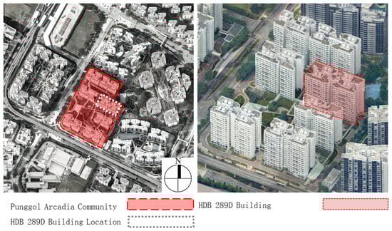
Figure 11.
The building planning details.
According to previous research, the size of the residential unit was set at 3.2 m wide, 4.5 m deep, and 2.8 m high [50,51] (Figure 12). The prototype of the productive facade reflected the layout of the T2 Lab [52]. The upper part was a PV shading system (one-layer monocrystalline silicon or thin-film PV shading modules) with a tilt angle of 20°, considering the balance between the PV electricity yield and indoor light environment [9]. The area of the PV module was 2.56 m2 (0.8 m × 3.2 m), with the 0.8 m width of the PV module determined by the arrangement of four rows of 0.2 m PV cells to match the mainstream cell size development trend. The length of 3.2 m was the same as the width of the residential unit to maximize the potential of solar energy and improve the indoor environmental quality. Since the ANN prediction unit for the PV shading electricity yield was Wh/m2, the final yield used the ANN prediction result multiplied by the area of the PV module. The lower part was a vertical farming system with three rows of planting units that allow 36 vegetables to grow, and the interval between each row of planting units was 0.2 m to meet the growing space requirements of vegetables. The parapet behind the vertical farming system was replaced by a customized opening to allow access to the crops [16]. By installing a 3-layer planting unit on a rail that can slide up and down, the planting units can be maintained more conveniently. However, to simplify the model, an opaque wall was considered, as in the case of the T2 lab testbed. The parameter settings of the residential unit were set according to the GreenMark [52], and the layout parameters of the building planning are detailed in Figure 12 and Figure 13.
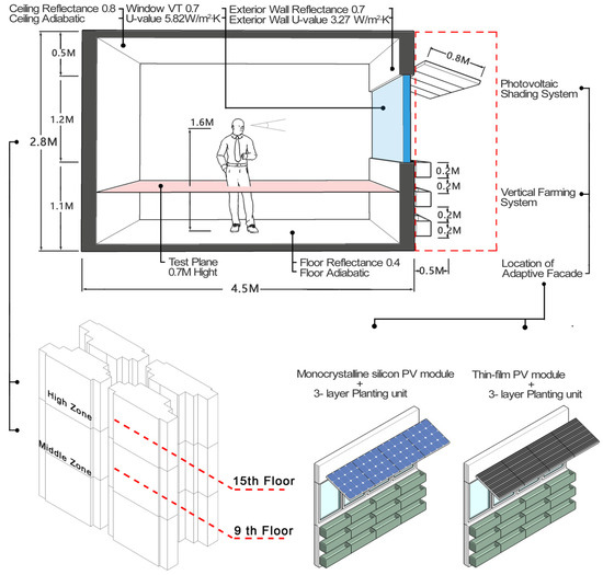
Figure 12.
The residential unit.
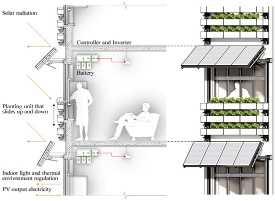
Figure 13.
Sectional and Front view of Productive facade.
3. Results
First of all, using experimental data training and testing ANN to generate prediction results, which, when compared to the experimental results, testify that the prediction models using the Bipolar Sigmoid activation function fit the experimental data better (R2 = 0.88 for electricity yield and R2 = 0.63 for vegetable yields) than SoftPlus (R2 = 0.78 for electricity yield and R2 = 0.61 for vegetable yields) and MLR (R2 = 0.52 for electricity yield and R2 = 0.47 for vegetable yields). Therefore, the ANN-used Bipolar Sigmoid activation function is selected as the productive façade yield prediction model.
Then, this prediction model was applied in a case to evaluate the electricity and vegetable yields of the productive facade in the high and middle zones of a building facade facing the SSW. Using the Rhinoceros with Grasshopper plug-in platform, the prediction model obtained the annual PV shading electricity yield and annual vertical farming vegetable yield in the high and middle zones of the residential model (Table 12). In general, the yields in the high zone were higher than those in the middle zone. The yield of the monocrystalline silicon PV module was higher than that of the thin-film PV module.
Table 12.
Index comparison.
For the PV electricity yield, the annual electricity yield of the monocrystalline silicon and thin-film PV modules was 274.3 and 237.8 kWh in the high zone and 251.4 and 218.3 kWh in the middle zone, respectively. According to the Singapore Bureau of Statistics, the average monthly household electricity consumption of public housing in 2020 was 395.6 kWh (for four-bedroom residences) [53]. According to the above data, the output of the productive facade can meet 23.1% (using a monocrystalline silicon PV module) or 20.0% (using a thin-film PV module) of the annual electricity demand from residential units composed of four-room residential units in the high zone. The middle zone can meet 21.2% (using a monocrystalline silicon PV module) or 18.4% (using a thin-film PV module) of the annual electricity demand.
In terms of vertical farming vegetable yield, the annual yield of a single residential unit in the high zone was 19.8 kg dry weight (calculated based on the average value of 73–95% of the moisture in leafy vegetables; 19.8 kg dry weight is about 99 kg of fresh vegetable weight [54]), and a single residential unit’s annual yield in the middle zone was 17.1 kg dry weight (approximately 85.5 kg fresh vegetable weight). In 2014, the per capita consumption of leafy vegetables in Singapore was 96 kg [55]. For the common four-room residential units in Singapore, the annual vegetable self-sufficiency rate of a four-person household can reach 103% (high zone) or 89.1% (middle zone) after the application of a productive facade. This is crucial to Singapore, where the current vegetable self-sufficiency rate is only 13%, and almost 90% of all vegetables are imported [56].
4. Discussion and Conclusions
Based on the experimental data from the T2 Lab at NUS in Singapore, this paper developed a performance prediction method applied to ANN and presents the application of this method and the results of predicting the electricity and vegetable yield of a productive facade in a typical residential building in Singapore. First, based on different activation functions, an ANN was trained using the experimental data, and then the prediction models involving environmental and yield elements were built. Finally, due to the better performance of the other two activation functions, the yield prediction method of the productive facade was completed using ANN with the Bipolar Sigmoid activation function, which integrated the PV shading and vertical farming systems.
PV shading and vertical farming are increasingly being applied to architectural facade design and practice, but predicting PV electric energy and vertical farming vegetable yield is complex owing to the multitude of influencing parameters.
It should be noted that the integration of PV shading and vertical farming into building facades is a challenging task because of the need to consider compatibility between systems, urban shading effects, optimal design, architectural aesthetics, and so on. In the context of multi-objective decision-making, the optimal solution is often limited by the inability to obtain data on PV electricity yield and building facade vegetable output because these two are difficult to use with traditional methods such as simulation or formula derivation quickly and accurately. With PV shading and vertical farming being increasingly applied to building facade design and practice, the novel prediction method proposed in this research is helpful to solve the performance evaluation problem in the context of complex influencing factors. The novel and predictive ANN, based on the Rhinoceros and Grasshopper plug-in platforms, proposed in this paper allows designers to predict the yield performance of productive facades with similar layouts of PV shading and vertical farming systems. A relatively reliable method for predicting the output of productive facade resources was obtained in different tropical urban contexts. In addition, researchers can obtain satisfactory design prototypes by comparing the performance of different productive facade prototypes to aid in the design decision-making process.
Future research will focus on different weather conditions, building types, materials, and crops, and improving the accuracy of predictions. Specifically, the prediction process and results of this study require further analysis and verification. As the training data, namely the experimental data, were obtained from Singapore, the prediction model is currently only applicable in regions close to the equator. Moreover, considering the prediction process, different PV installation environments affect the temperature of the PV modules differently, which in turn affects the PV electricity yield. This paper discusses the electricity yield of PV shading in the facade installation environment of residential buildings only. In this research, we found that the prediction results of machine learning represented by the ANN might have “jumping points”, i.e., a small number of prediction results had large errors. Therefore, in this study, for the same situation, the prediction model was used to conduct multiple rounds of prediction, and the data with large errors were excluded by comparing the prediction results, but the time cost of the prediction process was also increased to a certain extent. Therefore, it is necessary to find ways to improve the predictive model from the perspective of tool iteration or algorithm updates.
CIGS thin-film was selected for this study, and more thin-film PV module types will be conducted. Finally, considering crop yield prediction, the experiment focused on shade-loving crops (lettuce) that make full use of low-light conditions. Therefore, the yield prediction of other crop types is another avenue for future research.
The next step is to examine how predictive models can be packaged and integrated into the current building facade design process. Through the application of measurement and satisfaction surveys, the prediction model is constantly improved, and a shared platform is built among designers, users, and manufacturers to achieve a balance between performance, user satisfaction, cost, and architectural aesthetics.
Energy and food security have always been bottlenecks in sustainable urban development. Through the rational use of solar energy resources, the productive facade, which integrates PV shading and vertical farming systems, provides feasible solutions for improving the quality of urban human settlements and promoting the development of urban green energy and food security.
Author Contributions
Conceptualization, A.T.; methodology, X.S.; software, X.S.; validation, X.M.; investigation, A.T.; resources, A.T.; writing—review and editing, X.S. and L.W.; visualization, W.H.; supervision, L.W. All authors have read and agreed to the published version of the manuscript.
Funding
This study was funded by the Natural Science Foundation of Shandong Province (ZR202209150015), National Key Research and Development Program of China (Grant No. 2023YFC3807404-3), and the China Scholarship Council, as well as partially financed by the Department of Architecture, School of Design and Environment, National University of Singapore (NUS). Data were obtained from the NUS-CDL Tropical Technologies Laboratory (T2 Lab) at NUS. We are grateful for the collaboration with members of the T2 Lab, namely Stephen Siu-Yu Lau, Siu-Kit Lau, Yuan Chao, Huang Huajing, and Ian K. Chaplin. The settings and analysis of the vertical farming system were conducted in collaboration with Hugh Tan, Song Shuang, and the team from the Department of Biological Sciences, NUS. The settings and data recording were conducted in collaboration with Veronika Shabunko, Thomas Reindl, and the team from the Solar Energy Research Institute of Singapore (SERIS). The farming and irrigation systems were partially financed by UNISEAL®.
Data Availability Statement
The data presented in this study are available on request from the corresponding author. The data are not publicly available because the research is still going on.
Conflicts of Interest
The authors declare no conflicts of interest.
Appendix A
Table A1.
Schedule for T2 lettuce cultivation *.
Table A1.
Schedule for T2 lettuce cultivation *.
| Date | Batch | Day | Activity | Date | Batch | Day | Activity |
|---|---|---|---|---|---|---|---|
| 06/12/2018 | 1 | 0 | Sow seeds | 26/03/2019 | 4 | 14 | Transplant |
| 20/12/2018 | 1 | 14 | Transplant | 29/03/2019 | 4 | 17 | Fertilize |
| 23/12/2018 | 1 | 17 | Fertilize | 08/04/2019 | 4 | 27 | Fertilize |
| 02/01/2019 | 1 | 27 | Fertilize | 13/04/2019 | 5 | 0 | Sow seeds |
| 07/01/2019 | 2 | 0 | Sow seeds | 18/04/2019 | 4 | 37 | Fertilize |
| 12/01/2019 | 1 | 37 | Fertilize | 26/04/2019 | 4 | 45 | Harvest |
| 20/01/2019 | 1 | 45 | Harvest | 27/04/2019 | 5 | 14 | Transplant |
| 21/01/2019 | 2 | 14 | Transplant | 30/04/2019 | 5 | 17 | Fertilize |
| 24/01/2019 | 2 | 17 | Fertilize | 10/05/2019 | 5 | 27 | Fertilize |
| 03/02/2019 | 2 | 27 | Fertilize | 13/05/2019 | 6 | 0 | Sow seeds |
| 08/02/2019 | 3 | 0 | Sow seeds | 20/05/2019 | 5 | 37 | Fertilize |
| 13/02/2019 | 2 | 37 | Fertilize | 28/05/2019 | 5 | 45 | Harvest |
| 21/02/2019 | 2 | 45 | Harvest | 29/05/2019 | 6 | 14 | Transplant |
| 22/02/2019 | 3 | 14 | Transplant | 01/06/2019 | 6 | 17 | Fertilize |
| 25/02/2019 | 3 | 17 | Fertilize | 11/06/2019 | 6 | 27 | Fertilize |
| 07/03/2019 | 3 | 27 | Fertilize | 21/06/2019 | 6 | 37 | Fertilize |
| 12/03/2019 | 4 | 0 | Sow seeds | 29/06/2019 | 6 | 45 | Harvest |
| 17/03/2019 | 3 | 37 | Fertilize | ||||
| 25/03/2019 | 3 | 45 | Harvest |
* Note: This information was provided by Song Shuang and the team from the Department of Biological Sciences at NUS.
Table A2.
Planting data record sheet.
Table A2.
Planting data record sheet.
| Average DLI (mol/m2d) | Time Proportion of the Suitable Illumination | Soil Fertility | Average Dry Weight per Plant (Unit: g) | |
|---|---|---|---|---|
| 6 rounds of planting data in the east | 8.16 | 19.42% | 1 | 42.00 |
| 5.83 | 7.95% | 0.9 | 38.00 | |
| 6.75 | 10.77% | 0.8 | 33.81 | |
| 5.94 | 9.25% | 0.7 | 19.82 | |
| 6.04 | 7.66% | 0.6 | 13.40 | |
| 5.58 | 8.10% | 1 | 16.97 | |
| 6 rounds of planting data in the south | 5.71 | 2.85% | 0.7 | 20.84 |
| 5.17 | 1.25% | 0.6 | 9.26 | |
| 5.29 | 0.10% | 1 | 14.40 | |
| 6 rounds of planting data in the west | 7.21 | 14.70% | 1 | 36.05 |
| 4.41 | 2.60% | 0.9 | 27.83 | |
| 4.49 | 2.20% | 0.8 | 21.53 | |
| 4.51 | 2.79% | 0.7 | 11.66 | |
| 5.89 | 8.17% | 0.6 | 13.65 | |
| 6.34 | 8.05% | 1 | 28.02 | |
| 6 rounds of planting data in the north | 4.63 | 0.00% | 1 | 25.35 |
| 5.29 | 0.00% | 0.9 | 22.89 | |
| 6.32 | 1.06% | 0.8 | 20.04 | |
| 7.76 | 9.58% | 0.7 | 23.63 | |
| 8.76 | 15.78% | 0.6 | 26.29 | |
| 9.38 | 18.19% | 1 | 23.28 |
Notes: The unit of DLI is mol/m2d, the proportion of suitable illumination is defined as the time proportion of not less than 14 mol/m2d, that is 324 umol/m2/s during the day (6 a.m.–18 p.m.). The Soil fertility of the number of rounds showed a decreasing distribution of equal difference. The initial value was set to 1, and the unit of average dry weight per plant was grams. The data were provided by Song Shuang and the team from the Department of Biological Sciences at NUS.
Table A3.
Neural network training data and test data (monocrystalline silicon PV module).
Table A3.
Neural network training data and test data (monocrystalline silicon PV module).
| Independent Variables | Dependent Variables | ||||
|---|---|---|---|---|---|
| Ambient Temperature °C | Wind Speed m/s | GHI on the Roof W/m2 | PV Module Incident Solar Radiation W/m2 | PV Module Temperature °C | PV Module Output Power W/m2 |
| 28.56 | −0.04 | 2.95 | 1.56 | 24.71 | 0.00 |
| 29.72 | 0.06 | 118.52 | 77.74 | 29.22 | 15.75 |
| 29.26 | −0.04 | 2.78 | 1.56 | 25.10 | 0.00 |
| 31.37 | 0.15 | 584.15 | 458.87 | 55.04 | 40.35 |
| 28.87 | 1.45 | 2.74 | 1.57 | 25.85 | 0.00 |
| 30.85 | −0.04 | 457.74 | 84.22 | 34.92 | 19.69 |
| 31.33 | −0.04 | 281.93 | 54.93 | 30.07 | 9.84 |
| 28.73 | −0.04 | 2.81 | 1.55 | 24.94 | 0.00 |
| 30.90 | −0.04 | 83.27 | 65.79 | 33.76 | 10.83 |
| 30.02 | −0.04 | 49.69 | 32.99 | 29.91 | 4.92 |
| 29.68 | −0.04 | 3.32 | 1.59 | 27.19 | 0.00 |
| 29.09 | 0.62 | 70.54 | 24.01 | 27.31 | 3.94 |
| 29.53 | 0.93 | 138.61 | 41.27 | 27.48 | 5.91 |
| 29.57 | −0.04 | 3.05 | 1.59 | 27.16 | 0.00 |
| 29.01 | −0.04 | 2.81 | 1.56 | 25.62 | 0.00 |
| 29.11 | −0.04 | 3.13 | 1.58 | 25.73 | 0.00 |
| 31.41 | 0.23 | 567.92 | 709.11 | 56.06 | 0.98 |
| 29.50 | −0.04 | 3.11 | 1.58 | 26.49 | 0.00 |
| 28.93 | −0.04 | 11.36 | 8.25 | 26.32 | 0.00 |
| 29.35 | −0.04 | 3.03 | 1.56 | 25.37 | 0.00 |
| 29.73 | −0.04 | 3.14 | 1.59 | 27.34 | 0.00 |
| 30.40 | −0.04 | 273.75 | 39.89 | 28.38 | 6.89 |
| 30.01 | 0.70 | 176.63 | 112.55 | 33.01 | 19.69 |
| 30.71 | −0.04 | 3.67 | 1.62 | 29.50 | 0.00 |
| 30.24 | 0.36 | 429.86 | 384.07 | 43.07 | 75.79 |
| 28.83 | −0.04 | 3.08 | 1.56 | 25.59 | 0.00 |
| 28.68 | −0.04 | 22.81 | 10.41 | 24.90 | 0.98 |
| 31.20 | 0.44 | 621.97 | 65.70 | 34.14 | 19.69 |
| 28.84 | −0.04 | 2.88 | 1.57 | 26.64 | 0.00 |
| 29.96 | 0.28 | 288.51 | 189.30 | 34.34 | 40.35 |
| 30.79 | 0.97 | 880.54 | 557.85 | 57.11 | 62.01 |
| 30.22 | 0.02 | 17.43 | 13.38 | 30.17 | 1.97 |
| 29.97 | 2.07 | 389.25 | 257.82 | 39.11 | 54.13 |
| 29.15 | −0.04 | 40.00 | 27.46 | 27.54 | 3.94 |
| 28.92 | −0.04 | 30.46 | 16.57 | 24.84 | 1.97 |
| 29.04 | −0.04 | 2.83 | 1.56 | 26.18 | 0.00 |
| 29.40 | −0.04 | 2.94 | 1.58 | 27.70 | 0.00 |
| 30.69 | −0.04 | 297.37 | 209.80 | 38.93 | 44.29 |
| 31.29 | 0.27 | 516.58 | 65.15 | 37.18 | 10.83 |
| 30.96 | −0.02 | 305.42 | 194.68 | 40.83 | 42.32 |
| 29.65 | 0.68 | 157.06 | 166.15 | 32.49 | 26.57 |
| 32.03 | −0.04 | 769.95 | 662.31 | 46.31 | 67.91 |
| 29.52 | −0.04 | 3.07 | 1.58 | 26.60 | 0.00 |
| 29.60 | −0.04 | 11.55 | 6.34 | 25.94 | 0.00 |
| 31.82 | 0.02 | 643.68 | 131.63 | 37.32 | 30.51 |
There are 65,880 sets of training data and test data. Some variables are not involved in the final training procession. Due to space reasons, only 45 sets are shown here.
Table A4.
Neural network training data and test data (thin-film PV module).
Table A4.
Neural network training data and test data (thin-film PV module).
| Independent Variables | Dependent Variables | ||||
|---|---|---|---|---|---|
| Ambient Temperature °C | Wind Speed m/s | GHI on the Roof W/m2 | PV Module Incident Solar Radiation W/m2 | PV Module Temperature °C | PV Module Output Power W/m2 |
| 29.37 | −0.02 | 2.99 | 0.22 | 26.87 | 0.00 |
| 30.48 | 0.71 | 10.77 | 2.88 | 30.30 | 0.00 |
| 30.29 | −0.04 | 251.37 | 230.89 | 35.93 | 88.42 |
| 30.03 | 1.12 | 161.88 | 67.35 | 34.20 | 32.84 |
| 30.57 | 0.89 | 466.46 | 288.63 | 49.10 | 135.16 |
| 30.18 | 0.72 | 314.05 | 32.00 | 29.98 | 16.42 |
| 29.89 | −0.02 | 93.95 | 26.84 | 29.16 | 11.37 |
| 30.01 | −0.04 | 3.38 | 0.43 | 28.72 | 0.00 |
| 30.46 | 0.03 | 240.57 | 95.15 | 38.39 | 50.53 |
| 30.93 | 0.21 | 139.88 | 50.57 | 35.26 | 22.74 |
| 29.37 | −0.04 | 220.89 | 142.46 | 38.57 | 70.74 |
| 30.69 | 0.25 | 6.59 | 1.76 | 30.44 | 0.00 |
| 27.65 | −0.05 | 33.77 | 18.13 | 24.84 | 5.05 |
| 29.34 | −0.04 | 2.98 | 0.41 | 26.84 | 0.00 |
| 29.66 | 0.04 | 337.70 | 188.86 | 43.24 | 103.58 |
| 29.75 | 0.27 | 83.80 | 44.60 | 32.49 | 20.21 |
| 30.14 | 0.12 | 229.97 | 64.23 | 33.52 | 35.37 |
| 28.99 | −0.05 | 2.92 | 0.40 | 25.13 | 0.00 |
| 29.73 | −0.04 | 11.88 | 4.08 | 26.54 | 0.00 |
| 29.49 | −0.02 | 3.01 | 0.27 | 26.81 | 0.00 |
| 31.44 | 1.37 | 578.52 | 256.40 | 58.13 | 101.06 |
| 29.34 | −0.02 | 3.08 | 0.22 | 26.88 | 0.00 |
| 29.31 | 0.19 | 216.63 | 110.67 | 29.12 | 58.11 |
| 29.89 | −0.02 | 3.03 | 0.22 | 27.34 | 0.00 |
| 30.49 | −0.02 | 3.73 | 0.26 | 30.16 | 0.00 |
| 30.78 | 0.01 | 303.92 | 228.74 | 38.44 | 114.95 |
| 30.75 | 0.16 | 408.07 | 159.43 | 41.55 | 92.21 |
| 30.66 | 0.56 | 417.17 | 32.78 | 35.86 | 17.68 |
| 30.15 | −0.05 | 3.22 | 0.42 | 27.57 | 0.00 |
| 31.03 | 0.12 | 344.52 | 259.14 | 51.78 | 10.11 |
| 29.09 | −0.05 | 3.08 | 0.41 | 25.66 | 0.00 |
| 27.81 | −0.05 | 59.57 | 43.91 | 26.97 | 18.95 |
| 31.34 | 0.16 | 723.94 | 44.02 | 33.41 | 21.47 |
| 29.61 | −0.02 | 3.35 | 0.21 | 26.16 | 0.00 |
| 28.93 | 0.13 | 2.92 | 0.20 | 25.91 | 0.00 |
| 29.40 | −0.01 | 3.01 | 0.42 | 26.44 | 0.00 |
| 31.53 | 0.00 | 838.47 | 520.87 | 71.12 | 66.95 |
| 30.82 | −0.02 | 246.84 | 79.76 | 36.41 | 40.42 |
| 30.17 | 0.46 | 240.29 | 80.80 | 35.25 | 22.74 |
| 29.59 | −0.02 | 3.22 | 0.22 | 26.88 | 0.00 |
| 28.43 | 0.07 | 2.59 | 0.39 | 25.52 | 0.00 |
| 29.81 | 1.23 | 362.59 | 145.96 | 40.22 | 30.32 |
| 31.33 | 0.35 | 692.35 | 535.13 | 61.90 | 138.95 |
| 31.68 | 0.27 | 354.55 | 151.15 | 47.01 | 98.53 |
| 29.66 | −0.05 | 3.01 | 0.40 | 26.55 | 0.00 |
There are 43,920 sets of training data and test data. Some variables are not involved in the final training. Due to space reasons, only 45 sets are shown here.
Table A5.
Neural network training data and test data (Vegetable yield).
Table A5.
Neural network training data and test data (Vegetable yield).
| Independent Variables | Dependent Variables | ||
|---|---|---|---|
| Average DLI (mol/m2d) | Time Proportion of the Suitable Illumination | Soil Fertility | Average Dry Weight per Plant (g) |
| 4.63 | 0.00 | 1.00 | 25.35 |
| 6.32 | 0.01 | 0.80 | 20.04 |
| 7.21 | 0.15 | 1.00 | 36.05 |
| 6.04 | 0.08 | 0.60 | 13.40 |
| 4.41 | 0.03 | 0.90 | 27.83 |
| 5.17 | 0.01 | 0.60 | 9.26 |
| 7.76 | 0.10 | 0.70 | 23.63 |
| 5.29 | 0.00 | 0.90 | 22.89 |
| 9.38 | 0.18 | 1.00 | 23.28 |
| 5.94 | 0.09 | 0.70 | 19.82 |
| 6.34 | 0.08 | 1.00 | 28.02 |
| 5.83 | 0.08 | 0.90 | 38.00 |
| 8.76 | 0.16 | 0.60 | 26.29 |
| 5.71 | 0.03 | 0.70 | 20.84 |
| 4.49 | 0.02 | 0.80 | 21.53 |
| 6.75 | 0.11 | 0.80 | 33.81 |
| 5.29 | 0.00 | 1.00 | 14.40 |
| 4.51 | 0.03 | 0.70 | 11.66 |
| 5.89 | 0.08 | 0.60 | 13.65 |
| 5.58 | 0.08 | 1.00 | 16.97 |
| 8.16 | 0.19 | 1.00 | 42.00 |
There are 21 sets of training data and test data.
References
- Sodiq, A.; Baloch, A.A.B.; Khan, S.A.; Sezer, N.; Mahmoud, S.; Jama, M.; Abdelaal, A. Towards modern sustainable cities: Review of sustainability principles and trends. J. Clean. Prod. 2019, 227, 972–1001. [Google Scholar] [CrossRef]
- International Energy Agency. IEA World Energy Statistics and Balances. 2017. Available online: https://www.oecd-ilibrary.org/energy/data/iea-world-energy-statistics-and-balances_enestats-data-en (accessed on 25 May 2021). [CrossRef]
- Young, R.; Hayes, S.; Kelly, M.; Vaidyanathan, S.; Kwatra, S.; Cluett, R.; Herndon, G. The 2014 International Energy Efficiency Scorecard[R/OL]//Report I1801; American Council for an Energy-Efficient Economy: Washington, DC, USA, 2014; Available online: http://aceee.org/research-report/u1408 (accessed on 25 May 2021).
- Chua, K.J.; Chou, S.K. Energy performance of residential buildings in Singapore. Energy 2010, 35, 667–678. [Google Scholar] [CrossRef]
- Pirog, R.; Van Pelt, T.; Enshayan, K.; Cook, E. Food, Fuel, and Freeways: An Iowa Perspective on How Far Food Travels, Fuel Usage, and Greenhouse Gas Emissions. Leopold Center for Sustainable Agriculture. Available online: http://171.67.100.116/courses/2016/ph240/swafford2/docs/pirog.pdf (accessed on 25 May 2021).
- Tong, D.; Crosson, C.; Zhong, Q.; Zhang, Y. Optimize urban food production to address food deserts in regions with restricted water access. Landsc. Urban Plan. 2020, 202, 103859. [Google Scholar] [CrossRef]
- Sky Greens. 2021. Available online: https://www.skygreens.com/about-skygreens/ (accessed on 26 May 2021).
- Al-Kodmany, K. The vertical farm: A review of developments and implications for the vertical city. Buildings 2018, 8, 24. [Google Scholar] [CrossRef]
- Tablada, A.; Kosorić, V.; Huang, H.; Chaplin, I.K.; Lau, S.K.; Yuan, C.; Lau, S.S.Y. Design optimisation of productive Façades: Integrating photovoltaic and farming systems at the tropical technologies laboratory. Sustainability 2018, 10, 3762. [Google Scholar] [CrossRef]
- Tablada, A.; Kosorić, V. Vertical Farming on Facades: Transforming Building Skins for Urban Food Security. In Rethinking Building Skins: Transformative Technologies and Research Trajectories; Gasparri, E., Brambilla, A., Lobaccaro, G., Goia, F., Andaloro, A., Sangiorgio, A., Eds.; Woodhead Publishing: Sawston, UK, 2022. [Google Scholar]
- Loonen, R.C.; Rico-Martinez, J.M.; Favoino, F.; Brzezicki, M.; Ménézo, C.; La Ferla, G.; Aelenei, L.L. Design for façade adaptability–Towards a unified and systematic characterization. In Proceedings of the 10th Energy Forum-Advanced Building Skins, Bern, Switzerland, 28–29 October 2024. [Google Scholar]
- Gao, N.P.; Niu, J.L.; Perino, M.; Heiselberg, P. The airborne transmission of infection between flats in high-rise residential buildings: Tracer gas simulation. Build. Environ. 2008, 43, 1805–1817. [Google Scholar] [CrossRef] [PubMed]
- Reynders, G.; Nuytten, T.; Saelens, D. Potential of structural thermal mass for demand-side management in dwellings. Build. Environ. 2013, 64, 187–199. [Google Scholar] [CrossRef]
- Kosorić, V.; Lau, S.K.; Tablada, A.; Lau, S.S. General model of Photovoltaic (PV) integration into existing public high-rise residential buildings in Singapore–Challenges and benefits. Renew. Sustain. Energy Rev. 2018, 91, 70–89. [Google Scholar] [CrossRef]
- Kosorić, V.; Huang, H.; Tablada, A.; Lau, S.K.; Tan, H.T. Survey on the social acceptance of the productive façade concept integrating photovoltaic and farming systems in high-rise public housing blocks in Singapore. Renew. Sustain. Energy Rev. 2019, 111, 197–214. [Google Scholar] [CrossRef]
- Tablada, A.; Kosorić, V.; Huang, H.; Lau, S.S.; Shabunko, V. Architectural quality of the productive façades integrating photovoltaic and vertical farming systems: Survey among experts in Singapore. Front. Archit. Res. 2020, 9, 301–318. [Google Scholar] [CrossRef]
- Chakraborty, D.; Elzarka, H. Advanced machine learning techniques for building performance simulation: A comparative analysis. J. Build. Perform. Simul. 2019, 12, 193–207. [Google Scholar] [CrossRef]
- Ye, Z.; Nobre, A.; Reindl, T.; Luther, J.; Reise, C. On PV module temperatures in tropical regions. Sol. Energy 2013, 88, 80–87. [Google Scholar] [CrossRef]
- Hofer, J.; Groenewolt, A.; Jayathissa, P.; Nagy, Z.; Schlueter, A. Parametric analysis and systems design of dynamic photovoltaic shading modules. Energy Sci. Eng. 2016, 4, 134–152. [Google Scholar] [CrossRef]
- Tey, Y.S.; Li, E.; Bruwer, J.; Abdullah, A.M.; Brindal, M.; Radam, A.; Ismail, M.M.; Darham, S. The relative importance of factors influencing the adoption of sustainable agricultural practices: A factor approach for Malaysian vegetable farmers. Sustain. Sci. 2014, 9, 17–29. [Google Scholar] [CrossRef]
- Foucquier, A.; Robert, S.; Suard, F.; Stéphan, L.; Jay, A. State of the art in building modelling and energy performances prediction: A review. Renew. Sustain. Energy Rev. 2013, 23, 272–288. [Google Scholar] [CrossRef]
- Majumder, M. Artificial Neural Network. Netw. Complex Syst. 2015, 3, 49–54. [Google Scholar] [CrossRef]
- Vukorep, I.; Kotov, A. Machine learning in architecture: An overview of existing tools. In The Routledge Companion to Artificial Intelligence in Architecture; Routledge: London, UK, 2021; pp. 93–109. [Google Scholar]
- Gossard, D.; Lartigue, B.; Thellier, F. Multi-objective optimization of a building envelope for thermal performance using genetic algorithms and artificial neural network. Energy Build. 2013, 67, 253–260. [Google Scholar] [CrossRef]
- Magnier, L.; Haghighat, F. Multiobjective optimization of building design using TRNSYS simulations, genetic algorithm, and Artificial Neural Network. Build. Environ. 2010, 45, 739–746. [Google Scholar] [CrossRef]
- Sulaiman, S.; Rahman, T.A.; Musirin, I. Partial Evolutionary ANN for Output Prediction of a Grid-Connected Photovoltaic System. Int. J. Comput. Electr. Eng. 2009, 1, 40–45. [Google Scholar] [CrossRef]
- Ding, M.; Wang, L.; Bi, R. An ANN-based approach for forecasting the power output of photovoltaic system. Procedia Environ. Sci. 2011, 11, 1308–1315. [Google Scholar] [CrossRef]
- Mellit, A.; Pavan, A.M. A 24-h forecast of solar irradiance using artificial neural network: Application for performance prediction of a grid-connected PV plant at Trieste, Italy. Sol. Energy 2010, 84, 807–821. [Google Scholar] [CrossRef]
- Izgi, E.; Öztopal, A.; Yerli, B.; Kaymak, M.K.; Şahin, A.D. Short-mid-term solar power prediction by using artificial neural networks. Sol. Energy 2012, 86, 725–733. [Google Scholar] [CrossRef]
- Mellit, A.; Saǧlam, S.; Kalogirou, S.A. Artificial neural network-based model for estimating the produced power ofaphotovoltaic module. Renew. Energy 2013, 60, 71–78. [Google Scholar] [CrossRef]
- De Giorgi, M.G.; Congedo, P.M.; Malvoni, M. Photovoltaic power forecasting using statistical methods: Impact of weather data[J/OL]. IET Sci. Meas. Technol. 2014, 8, 90–97. [Google Scholar] [CrossRef]
- Almonacid, F.; Pérez-Higueras, P.J.; Fernández, E.F.; Hontoria, L. A methodology based on dynamic artificial neural network for short-term forecasting of the power output of a PV generator. Energy Convers. Manag. 2014, 85, 389–398. [Google Scholar] [CrossRef]
- Abrougui, K.; Gabsi, K.; Mercatoris, B.; Khemis, C.; Amami, R.; Chehaibi, S. Prediction of organic potato yield using tillage systems and soil properties by artificial neural network (ANN) and multiple linear regressions (MLR). Soil Tillage Res. 2019, 190, 202–208. [Google Scholar] [CrossRef]
- Saad, P.; Yaakob, S.N.; Rahaman, N.A.; Daud, S.; Bakri, A.; Kamarudin, S.; Ismail, N. Artificial Neural Network Modelling of Rice Yield Prediction in Precision Farming. Researchgate.Net. 2002. Available online: https://www.researchgate.net/profile/Nurulisma-Ismail-2/publication/267511857_Artificial_Neural_Network_Modelling_of_Rice_Yield_Prediction_in_Precision_Farming/links/55ded55408ae79830bb593f1/Artificial-Neural-Network-Modelling-of-Rice-Yield-Prediction-in- (accessed on 9 July 2021).
- Pantazi, X.E.; Moshou, D.; Alexandridis, T.; Whetton, R.L.; Mouazen, A.M. Wheat yield prediction using machine learning and advanced sensing techniques. Comput. Electron. Agric. 2016, 121, 57–65. [Google Scholar] [CrossRef]
- Khean, N.; Kim, L.; Martinez, J.; Doherty, B.; Fabbri, A.; Gardner, N.; Haeusler, M.H. The introspection of deep neural networks—Towards illuminating the black box: Training architects machine learning via grasshopper definitions. In Proceedings of the CAADRIA 2018—23rd International Conference on Computer-Aided Architectural Design Research in Asia: Learning, Prototyping and Adapting, Beijing, China, 17–19 May 2018; Volume 2, pp. 237–246. [Google Scholar]
- Alpaydin, E. Neural Networks and Deep Learning. In Machine Learning; MIT Press: Cambridge, MA, USA, 2021; Available online: https://www.academia.edu/download/62971418/neuralnetworksanddeeplearning20200415-115041-1t7vxpc.pdf (accessed on 9 July 2021).
- Shi, X.; Abel, T.; Wang, L. Influence of two motion types on solar transmittance and daylight performance of dynamic façades. Sol. Energy 2020, 201, 561–580. [Google Scholar] [CrossRef]
- Tablada, A.; Chaplin, I.; Huang, H.; Lau, S.; Yuan, C.; Lau, S.S.-Y. Simulation algorithm for the integration of solar and farming systems on tropical façades. In Proceedings of the 23rd International Conference of the Association for Computer-Aided Architectural Design Research in Asia (CAADRIA) 2018, Beijing, China, 17–19 May 2018; Volume 2, pp. 123–132. [Google Scholar]
- NUS. NUS DoA. 2019. Available online: https://www.sde.nus.edu.sg/arch/facilities/net-zero-energy-building-sde-4/ (accessed on 21 July 2021).
- Mcneel, R. Grasshopper Generative Modeling for Rhino. Computer Software. 2011. Available online: http://www.grasshopper3d.com (accessed on 24 December 2023).
- Mcneel, R. Rhinoceros. 2014. Available online: https://www.rhino3d.com (accessed on 24 December 2023).
- Akoglu, H. User’s guide to correlation coefficients. Turk. J. Emerg. Med. 2018, 18, 91–93. [Google Scholar] [CrossRef]
- Van Dao, D.; Adeli, H.; Ly, H.B.; Le, L.M.; Le, V.M.; Le, T.T.; Pham, B.T. A sensitivity and robustness analysis of GPR and ANN for high-performance concrete compressive strength prediction using a monte carlo simulation. Sustainability 2020, 12, 830. [Google Scholar] [CrossRef]
- Omar Nour-Eddine, I.; Lahcen, B.; Fahd, O.H.; Amin, B. Power forecasting of three silicon-based PV technologies using actual field measurements. Sustain. Energy Technol. Assess. 2021, 43, 100915. [Google Scholar] [CrossRef]
- Sit, V.; Poulin-Costello, M.; Bergerud, W. Catalog of Curves for Curve Fitting; Biometrics Information Handbook Series; Citeseer: Princeton, NJ, USA, 1994. [Google Scholar]
- Song, S.; Ee AW, L.; Tan, J.K.N.; Cheong, J.C.; Chiam, Z.; Arora, S.; Lam, W.N.; Tan, H.T.W. Upcycling food waste using black soldier fly larvae: Effects of further composting on frass quality, fertilising effect and its global warming potential. J. Clean. Prod. 2021, 288, 125664. [Google Scholar] [CrossRef]
- Lan, L.; Wood, K.L.; Yuen, C. A holistic design approach for residential net-zero energy buildings: A case study in Singapore. Sustain. Cities Soc. 2019, 50, 101672. [Google Scholar] [CrossRef]
- Tablada, A.; Zhao, X. Sunlight availability and potential food and energy self-sufficiency in tropical generic residential districts. Solar Energy 2016, 139, 757–769. [Google Scholar] [CrossRef]
- Teoalida. HDB History, Photos and Floor Plan Evolution 1930s to 2010s—The World of Teoalida. 2019. Available online: https://www.teoalida.com/singapore/hdbfloorplans/ (accessed on 20 March 2021).
- Building and Construction Authority. HDB Precast Pictorial Guide. 2014. Available online: https://www.bca.gov.sg/Publications/BuildabilitySeries/others/HDB_Precast_pictorial_guide_BCA.pdf (accessed on 7 June 2021).
- Singapore Building and Construction Authority (BCA). Green Mark for Residential Buildings Technical Guide and Requirements. Available online: https://www1.bca.gov.sg/docs/default-source/docs-corp-buildsg/sustainability/gm-rb-2016-technical-guide-_rev010120.pdf?sfvrsn=c6fb9fe_2 (accessed on 24 December 2023).
- Energy Market Authority. Average Monthly Household Electricity Consumption by Dwelling Type. Available online: https://www.ema.gov.sg/resources/singapore-energy-statistics/chapter3 (accessed on 3 June 2021).
- Gupta, S.; Lakshmi, A.J.; Manjunath, M.N.; Prakash, J. Analysis of nutrient and antinutrient content of underutilized green leafy vegetables. LWT-Food Sci. Technol. 2005, 38, 339–345. [Google Scholar] [CrossRef]
- DOS. Singapore Department of Statistics (DOS)|Singstat Website. Available online: https://www.singstat.gov.sg/ (accessed on 25 May 2021).
- Li, H.B. Vegetable production, circulation and price change in Singapore. Mark. Econ. Price 2014, 31–34. [Google Scholar] [CrossRef]


Disclaimer/Publisher’s Note: The statements, opinions and data contained in all publications are solely those of the individual author(s) and contributor(s) and not of MDPI and/or the editor(s). MDPI and/or the editor(s) disclaim responsibility for any injury to people or property resulting from any ideas, methods, instructions or products referred to in the content. |
© 2023 by the authors. Licensee MDPI, Basel, Switzerland. This article is an open access article distributed under the terms and conditions of the Creative Commons Attribution (CC BY) license (https://creativecommons.org/licenses/by/4.0/).