Longitudinal Seismic Response of Metro Tunnels Crossing a Fault with Multi-Slip Surfaces

Abstract

There are multiple seismic fault zones near Xi’an in China, among which the Li Piedmont Fault has multiple slip surfaces. A 3D finite element dynamic Soil–Fault–Tunnel model was established based on the engineering background of the Xi’an Metro tunnel orthogonally crossing the Li Piedmont Fault. The input seismic loads used the Chi-Chi, El-Centro, and artificial seismic waves, and the latter was artificially synthesized based on seismic conditions and site conditions of actual engineering. The Chi-Chi seismic wave with larger PGV/PGA and wider acceleration-sensitive area is a near-field seismic wave, while the others are far-field seismic waves. The seismic loads were transformed into the equivalent nodal force on the boundary nodes of the model, and nonlinear dynamic calculation was carried out to obtain the longitudinal seismic response of the structure. The main results show that the fault amplifies the seismic response of the tunnel, and the tunnel at the position of the fault slip surfaces is more vulnerable to failure, especially near the slip surface between the hanging wall and the fault, where the maximum acceleration, soil pressure, and internal force of the tunnel structure occur. In addition, the seismic response of the tunnel and soil caused by near-field seismic motion is significantly stronger than that caused by far-field seismic motion.

1. Introduction

It is generally believed that the level of seismic damage to underground structures such as tunnels may be lower due to certain constraints of the surrounding rock. However, the level of seismic damage to underground structures such as tunnels may be more serious when they are near or cross the seismic fault [1,2,3]. The fault fracture zone directly affects the safety of the tunnel due to the poor surrounding rock conditions and insufficient self-stability. Seismicity is closely related to the distribution and activity of faults. Consequently, when the tunnel is near or crosses the seismic fault, the coupling effect of seismic action and strata change caused by fault activity can make the seismic damage mechanism to the tunnel more complicated.

Many scholars have researched the mechanism behind damage to tunnel-crossing faults and achieved relevant results [4,5,6,7,8,9,10,11,12,13,14,15,16,17,18,19]. For example, Mehdi Sabagh [14] conducted a 1:60 centrifuge test of a tunnel crossing an active normal fault, exploring the mechanism of tunnel failure and the process of crack development. Liu-Xuezeng et al. [15] conducted a model test of a tunnel crossing a 75° dip normal fault and concluded that the surrounding rock pressure would change significantly near the shear zone. Xu-Dingyu et al. [16] explored the relationship between the tunnel damage mechanism and fault distance, fault dip, and fault width through numerical simulation. Yang-Zhihua et al. [17] concluded that seismic motion and faults can change the initial stress field of the tunnel surrounding rock, resulting in stress accumulation and stress concentration in the tunnel surrounding rock near the fault and, ultimately, progressive destruction. Liu-Nina et al. [18] carried out shaking table model tests for a metro tunnel crossing active ground cracks. They studied the acceleration response, soil pressure, and strain variation of the metro tunnel under seismic action. Geng-Ping et al. [19] studied the equivalent strain response of highway tunnels crossing faults under seismic action using numerical analysis methods.

The above research provides a scientific basis for the seismic resistance and disaster reduction of tunnels crossing faults. However, the dynamic response characteristics such as acceleration, internal force, and soil pressure of metro tunnels crossing faults under seismic action still need further study. On the other hand, the seismic behavior of underground structures such as tunnels is mainly studied in terms of the lateral seismic response, and scholars have obtained fruitful research results and applied them in practical engineering design [20,21,22,23]. However, there is little research on longitudinal seismic behavior.

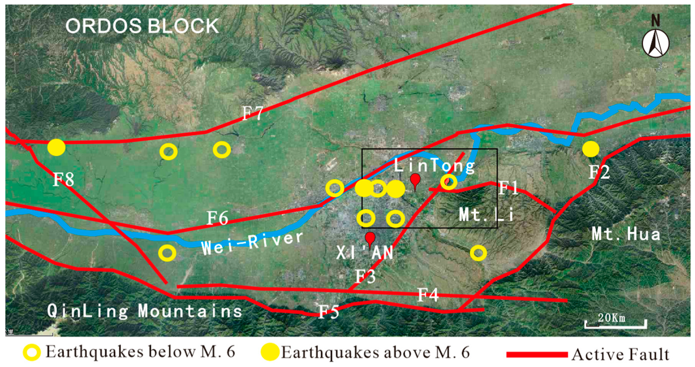
Xi’an, a megacity in China, is located at the intersection of multiple seismic zones, including the Qinghai–Tibet earthquake zone, the North China earthquake zone, and the South China earthquake zone. Consequently, seismicity in Xi’an is relatively active. There are multiple seismic faults distributed near Xi’an in the Wei River Basin, and there have been multiple earthquakes in history, including significant earthquakes of magnitude 6 or above (Figure 1). Multiple metro lines in Xi’an cross fault areas. Therefore, the seismic action and the impact of faults pose a severe threat to the safe operation of the metro tunnel.

Xi’an Metro Line 9, also known as the Lintong Line, inevitably crosses the Piedmont Fault of Li Mountain. This paper uses it as the research background to explore, through numerical simulation, the longitudinal seismic response of the tunnel crossing the fault. The research results can provide theoretical support and a scientific basis for the seismic response, damage mechanism, and seismic design of metro tunnels crossing multi-slip surface faults.

In this paper, Section 2 introduces the engineering background; Section 3 introduces the process of establishing a numerical calculation model; Section 4 introduces the seismic records used in dynamic research and analyzes their characteristics; Section 5 analyzes the calculation results; and Section 6 briefly discusses the research results and summarizes the research conclusions.

2. Engineering Background

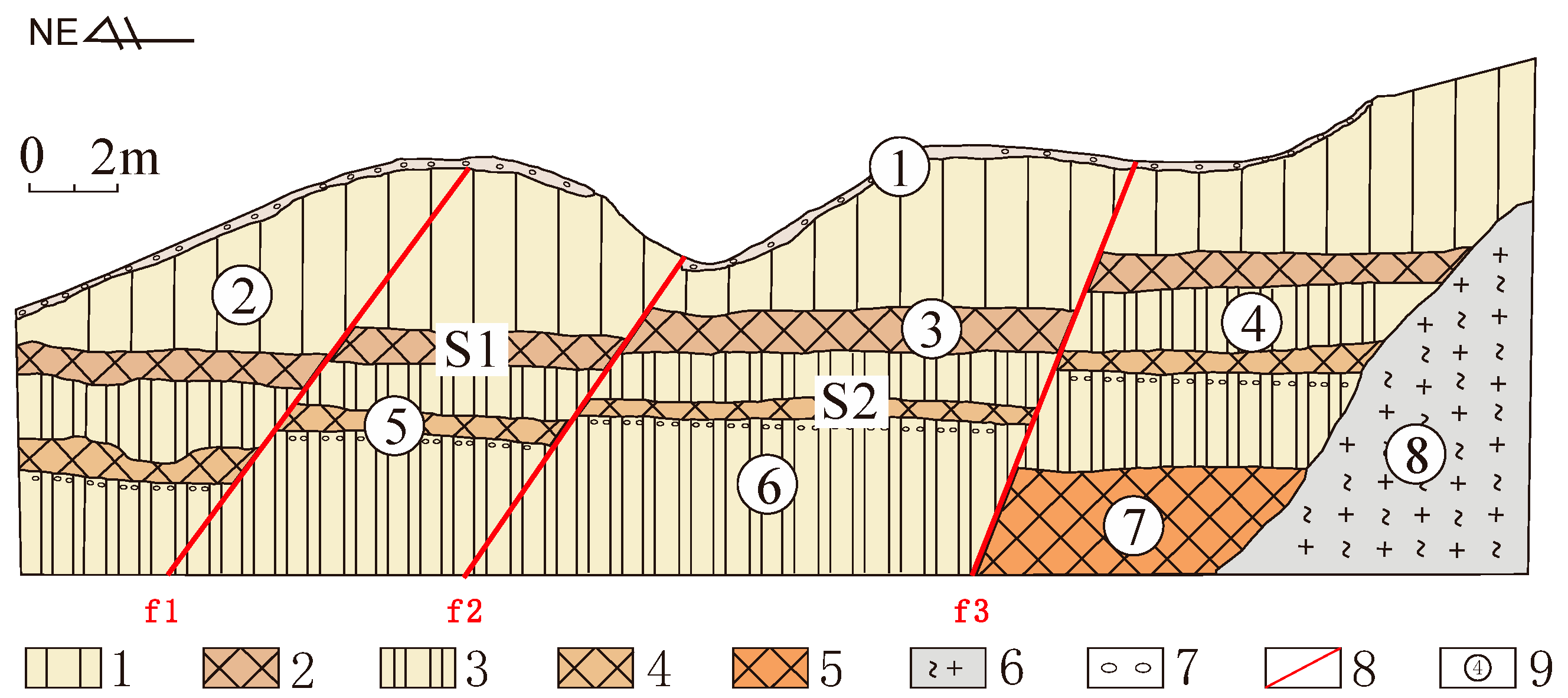
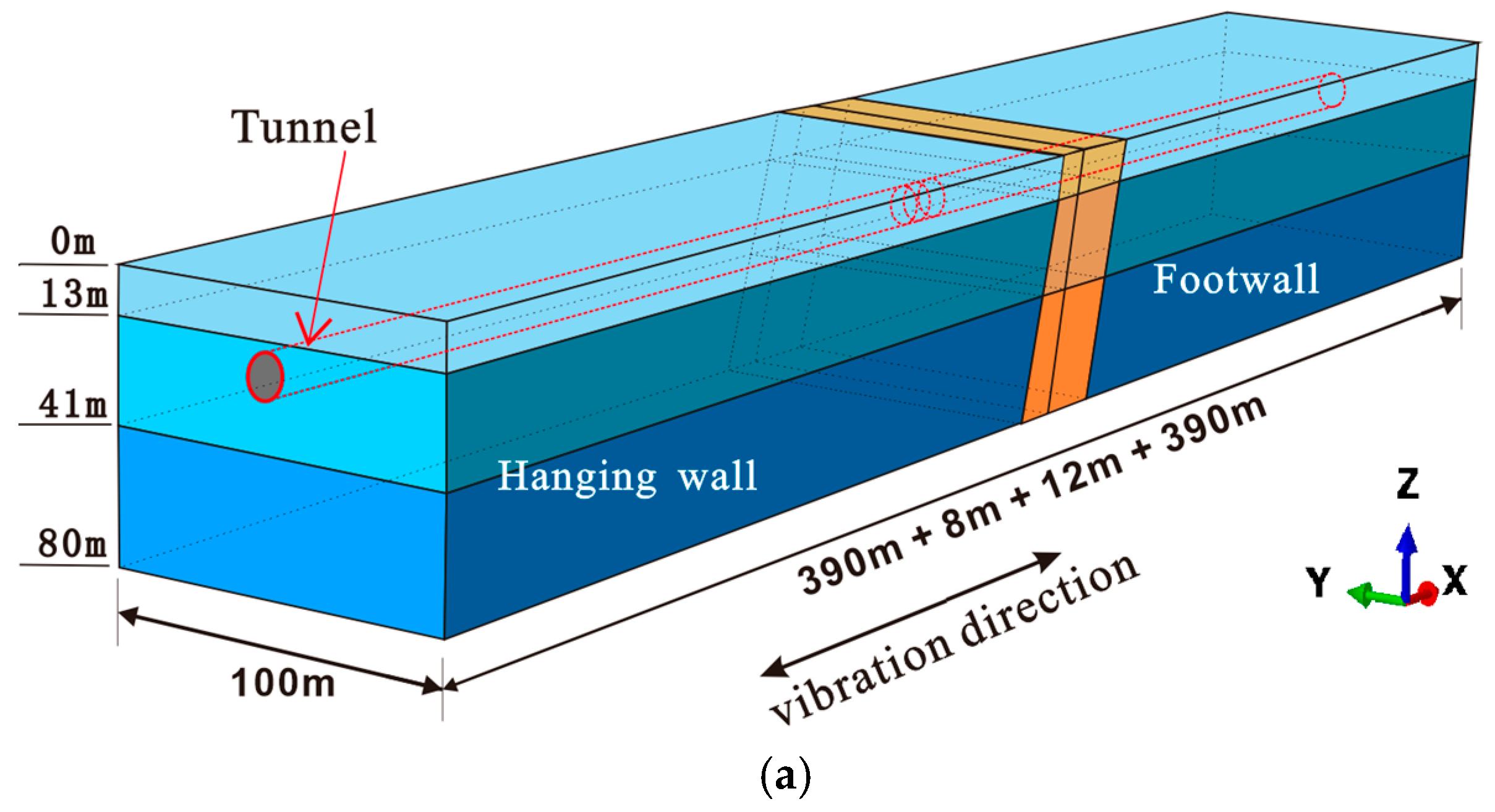
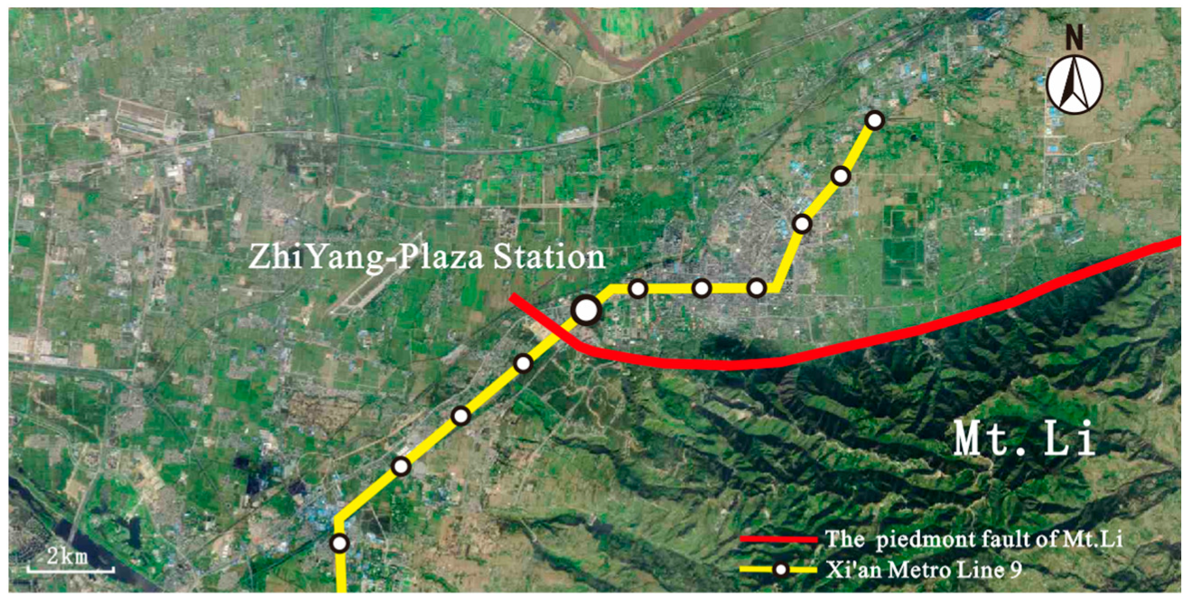
The total length of the Piedmont Fault of Li Mountain is about 40 km, the fault strike is near the west, the fault dip is about 75° to the north, and the fault has the characteristics of multi-slip surfaces (Figure 2) [24]. Xi’an Metro Line 9 crosses the Piedmont Fault of Li Mountain at nearly 90° near ZhiYang Plaza Station in Lintong District (Figure 3). The LinTong District is the crucial area of seismic fortification in Shaanxi Province, and its seismic fortification intensity is VIII.

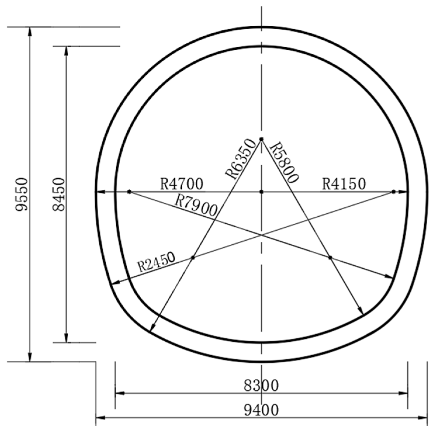
According to existing resources [25], Xi’an Metro Line 9 adopts shallow buried and hidden excavation construction methods, and the tunnel lining material is made of C35 concrete. The information on the tunnel section is shown in Figure 4. In the metro section near ZhiYang Plaza Station, the burial depth of the tunnel vault is 18 m, and the thickness of the covered soil layer above the bedrock is about 77 m. Information on the soil layer is given in

Table 1. Parameters of the actual soil layer.

Soil Layer	Weight (kNm−3)	Modulus of Elasticity (MPa)	Poisson’s Ratio (μ)	Shear Wave Velocity (ms−1)	Cohesion (KPa)	The Angle of Internal Friction (°)	Bottom Depth (m)
① Miscellaneous fill	16.7	10	0.35	126.3	15	17	1.5
② New loess	17.0	16	0.3	283.3	30	20	13.5
③ Paleosol	17.0	20	0.3	381.8	33	23	17.5
④ Old loess	17.0	23	0.3	367.2	37	23	41
⑤ Silty clay	19.1	27	0.3	433.7	37	25	75
⑥ Grit	19.5	50	0.28	499.2	0	35	77
⑦ Bedrock	20.5	200	0.25		200	35

.

3. Numerical Calculation Model

3.1. Geometric Model

In the paper, ABAQUS is used to establish a 3D calculation Tunnel–Fault–Soil model based on prototype engineering. To make the calculation easier to converge, the actual soil mass is simplified into a three-layer soil model based on the actual thickness ratio of each soil layer. The parameters of the model are given in

Table 2. Parameters of the model.

Soil Layer	Weight (kNm−3)	Modulus of Elasticity (MPa)	Poisson’s Ratio (μ)	Shear Wave Velocity (ms−1)	Cohesion (kPa)	The Angle of Internal Friction (°)	Bottom Depth (m)
The first layer of soil	17.0	16	0.3	283.3	30	20	13.5
The second layer of soil	17.0	22.5	0.3	369.3	35.8	23	41.0
The third layer of soil	19.1	27	0.3	433.7	37	25	80.0
Tunnel lining	25.0	31,500	0.2

.

Considering the influence of the model’s size and boundary in numerical simulation, the overall size of the model is length × width × height = 800 m × 100 m × 80 m. The three-layer soil model is established according to the soil layer information in Table 2. The fault zone is divided into two parts, with widths of 8 m and 12 m, respectively. There are three slip surfaces formed between the hanging wall, footwall, and the fault zones. In this paper, the slip surface between the hanging wall and the fault is called the first slip surface. The 3D model is shown in Figure 5.

The S8R thick shell element simulates the tunnel lining, and the C3D8R solid element simulates the soil mass. The constitutive relationship of tunnel lining adopts ideal elastic–plastic behavior, and the constitutive relationship of soil mass adopts Mohr–Coulomb behavior. The Coulomb Friction Model was chosen to indicate the relationship of the contact between soil and soil, as well as between soil and tunnel [26], with a friction coefficient of 0.3.

3.2. Dynamic Parameters

Under dynamic load with a short holding time and periodic changes in load size and direction, the change in soil strain lags behind the change in soil stress [27]. Therefore, the dynamic calculation of the model in this paper involves dynamic parameters. The dynamic elastic modulus ${(E}_d)$ and dynamic Poisson’s ratio ${(\mu }_d)$ of the soil are related to the shear-wave velocity $\left(v_s\right)$ and compression-wave velocity $\left(v_p\right)$ of the soil layer. Their relationship is shown in Equations (1) and (2), where α and β, as constants, are 0.95 and 1.3, respectively [27], and $\rho$ is the soil’s density. $v_p$ can be calculated using empirical Equation (3), where k takes a value of 1.765 [27]. Accordingly, the dynamic parameters of the soil can be calculated, as shown in

Table 3. Dynamic parameters of the soil layer.

Soil Layer	${\mathit{v}}_{\mathit{s}}$ (m/s)	${\mathit{v}}_{\mathit{p}}$ (m/s)	${\mathit{E}}_{\mathit{d}}$ (MPa)	${\mathit{\mu }}_{\mathit{d}}$
The first layer of the soil	283.30	446.60	301.58	0.21
The second layer of the soil	369.30	575.90	506.94	0.20
The third layer of the soil	433.70	677.90	787.40	0.20

.

$$E_d=\alpha \frac{\rho v_s^2(3v_p^2-4v_s^2)}{(v_p^2-v_s^2)},$$

(1)

$${\mu }_d=\beta \frac{(v_p^2-2v_s^2)}{2(v_p^2-v_s^2)},$$

(2)

$$v_p=k{v}_s^{0.98},$$

(3)

When seismic waves propagate in the soil medium, they are affected by damping, resulting in total energy attenuation [27,28]. In this paper, Rayleigh damping, commonly used in engineering, simulates the attenuation process. The Rayleigh damping matrix $\left[\mathrm{C}\right]$ is related to the stiffness matrix $\left[\mathrm{K}\right]$ and mass matrix $\left[\mathrm{M}\right]$, as shown in Equation (4).

$$\left[\mathrm{C}\right]=a\left[\mathrm{M}\right]+b\left[\mathrm{K}\right],$$

(4)

In the above formula, $a$ and $b$ represent the mass damping coefficient and the stiffness damping coefficient, respectively, which can be calculated by Equations (5) and (6) [27].

$$a=\frac{2{\omega }_1{\omega }_{2 }\left({\xi }_2{\omega }_2-{\xi }_1{\omega }_1\right)}{{\omega }_2^2-{\omega }_1^2},$$

(5)

$$b=\frac{2\left({\xi }_2{\omega }_2-{\xi }_1{\omega }_1\right)}{{\omega }_2^2-{\omega }_1^2},$$

(6)

In the above formula, ${\xi }_{\mathrm{1,2}}$ represents the damping ratio, with a value of 0.05 [28], and ${\omega }_{\mathrm{1,2}}$ can be calculated by Equation (7). In Equation (7), $f_1$ and $f_2$ represent the self-vibration frequencies of the 1st vibration mode and the 2nd vibration mode in the model, respectively. The self-vibration frequencies of the model can be extracted using modal analysis: $f_1$ = 0.98, $f_2$ = 1.29.

$${\omega }_{\mathrm{1,2}}=2\pi f_{\mathrm{1,2}}$$

(7)

Accordingly, the mass damping coefficient and stiffness damping coefficient can be calculated further: a = 0.35, b = 0.007.

3.3. Boundary and Seismic Waves Input Method

In this paper, a viscoelastic boundary, commonly used in dynamic analysis, simulates the damping effect of infinite foundation radiation. When the viscoelastic boundary entirely absorbs the scattered wave, the node of the artificial viscoelastic boundary is subjected to the seismic free-field motion [29], so the seismic action process can be transformed into the free-field motion process at the boundary node. Then, the free-field motion can be transformed into the equivalent nodal force on the boundary so as to realize the input of seismic loads. According to [30], to achieve batch operations of this process, a program was developed using the MATLAB-R2018a platform to automatically add viscoelastic boundaries and apply equivalent nodal forces of seismic loads to the boundaries in ABAQUS-2018.

4. Seismic Waves

4.1. Selection of Seismic Waves

The Port Hueneme Earthquake in the United States in 1957 first introduced the difference between near-field earthquakes and far-field earthquakes [31], and people began to pay attention to the damage of near-field earthquakes. The seismic damage mechanism of underground structures experiencing near-field seismic action is more complex [3,19]. Near-field seismic motion refers to regional seismic motion that cannot be ignored in the near-field and mid-field terms of the radiation waves from focus, as it is relatively close to the focus [32]. Generally, near-field seismic motion refers to ground motion with a fault distance of less than 20 km [33]. According to the map of fault distribution around Xi’an (Figure 1), there are several seismic faults distributed in Xi’an, and many large earthquakes have occurred. Therefore, this paper considers the impact of near-field earthquakes on the Xi’an Metro Tunnel. The Chi-Chi seismic wave recorded by TCU-068 station during the 1999 Chi-Chi Earthquake in Taiwan is taken as the near-field input seismic wave, and the fault distance of this seismic wave is 0.32 km.

In 1940, a seismograph located in El-Centro, southern California, USA, recorded a complete seismic wave for the first time, and it was named the El-Centro seismic wave. This paper also takes the El-Centro seismic wave as an input seismic wave.

Earthquakes are natural disaster events, and the selection of input seismic records to study earthquakes is an important issue [34,35]. Real seismic motion records are extremely important. The Chi-Chi seismic wave and El-Centro seismic wave are both real seismic records. However, this paper takes the “Xi’an Metro Tunnel” as the research background. Given this, this paper also selects the artificial seismic wave that was fitted based on seismic conditions and site conditions of actual engineering in Xi’an. In addition, it should be noted that the artificial seismic wave and the El-Centro seismic wave mentioned earlier are far-field seismic waves.

4.2. Characteristics of Seismic Waves

Existing seismic records indicate that near-field seismic motion often has strong velocity–pulse effects. Research by Geng-Ping et al. [19] suggests that a near-field seismic wave with a pulse has a larger velocity amplitude (PGV) and displacement amplitude (PGD), as well as a larger ratio of velocity amplitude to acceleration amplitude (PGV/PGA), and these factors can help evaluate the potential damage-causing power of seismic motion.

Research by Wang-Jingzhe et al. [36] suggests that the higher the PGV/PVA value of seismic motion, the more likely that the acceleration response spectrum of the seismic wave will have a wider acceleration-sensitive region, which will significantly change the seismic response characteristics of the structure and make the structure tend to exhibit a rigid response. The potential damage-causing power of the seismic motion with a wider acceleration-sensitive region will also be more significant.

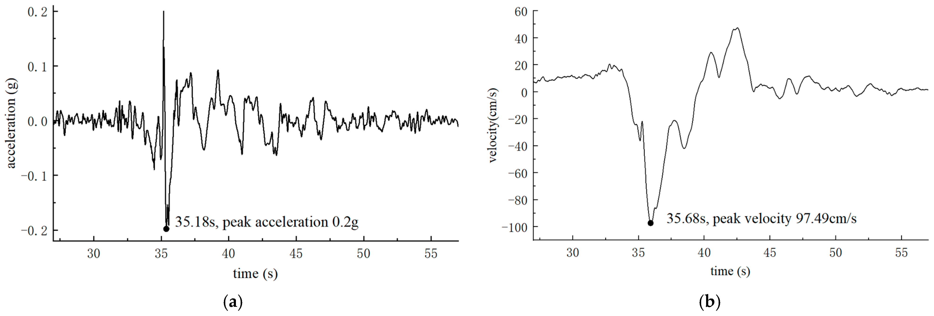
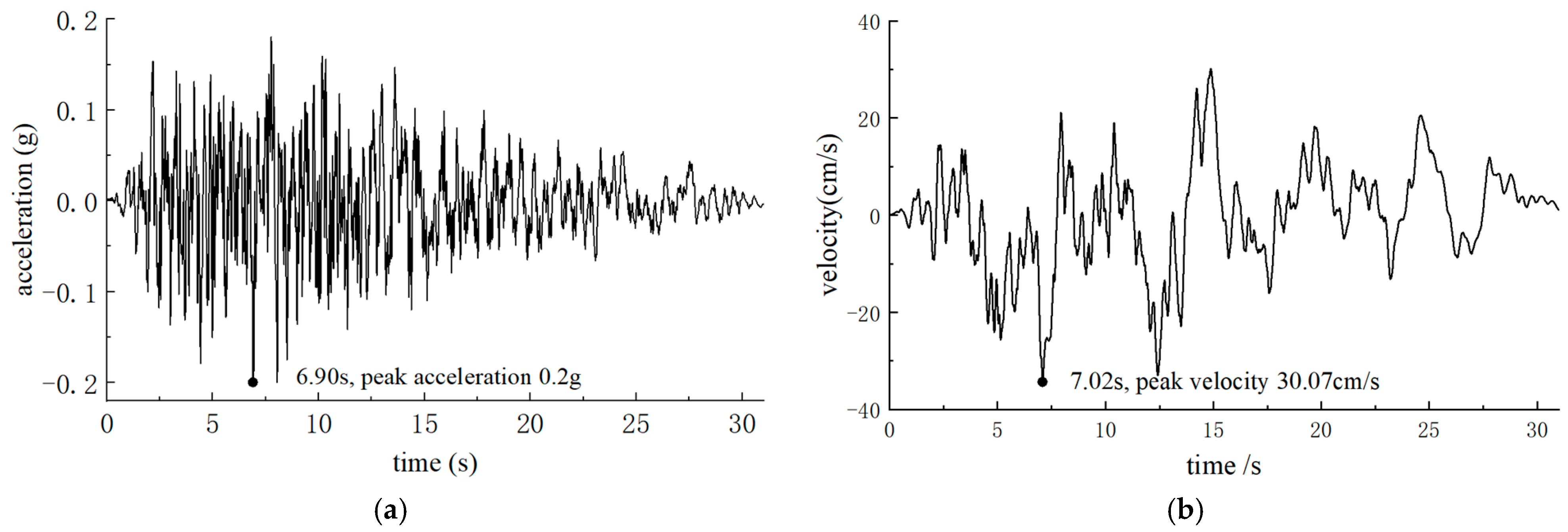
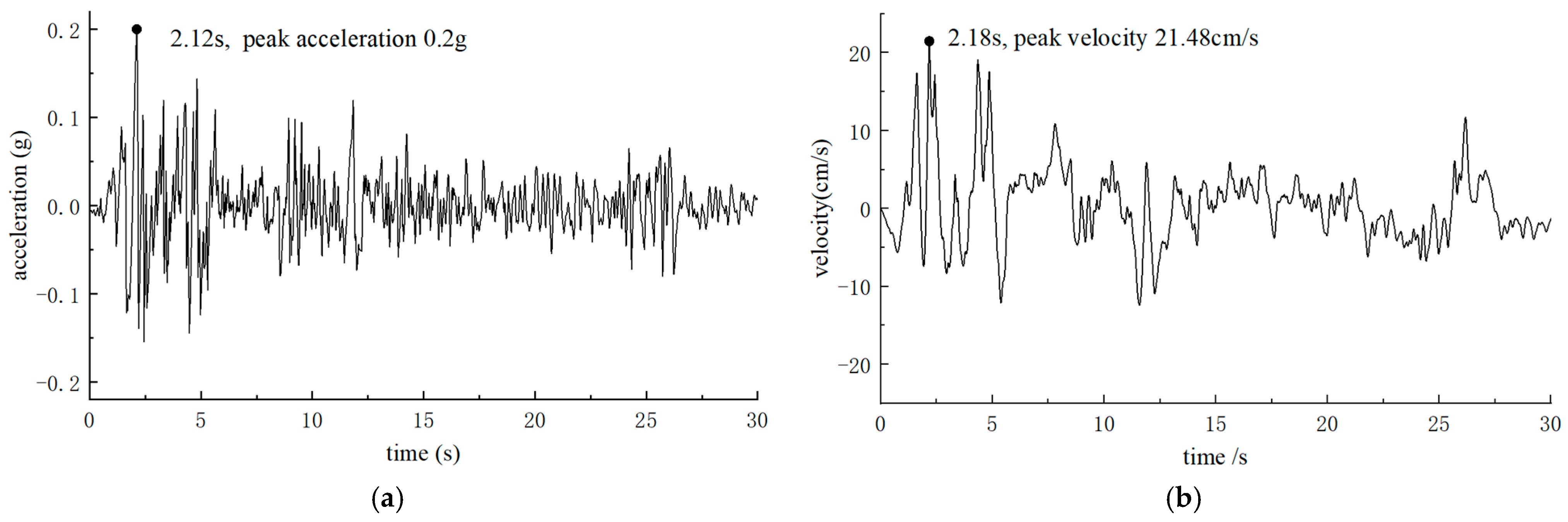
For the convenience of comparison, the selected seismic waves are uniformly adjusted in this paper: The acceleration amplitude of the seismic waves is uniformly adjusted to 0.2 g, which is the seismic fortification intensity of Xi’an; the seismic waves are filtered (the frequency is less than 15 Hz), and then the baseline correction is processed to reduce the drift error in the time–history of seismic acceleration measured by the strong seismograph. The time–history curves of velocity and displacement are obtained by integrating the adjusted acceleration time–history curve. To reduce the time required for dynamic calculation, this paper only captures the 30 s time–history, including the peak acceleration moment for the calculation.

In the case of unified amplitude modulation of acceleration to 0.2 g, the PGV of the Chi-Chi seismic wave, the artificial seismic wave, and the EI-Centro seismic wave are 97.49, 30.07, and 21.48 cm/s, respectively; the PGD values are 116.08, 70.11, and 24.31 cm, respectively; and the PGV/PGA values are 0.497, 0.131, and 0.109, respectively. It appears that the above indexes of the Chi-Chi seismic wave are much higher than those of other seismic waves.

The time–history curves of three seismic waves are shown in Figure 6, Figure 7 and Figure 8. The waveform characteristics of the time–history curves show that the peak acceleration and peak velocity of the Chi-Chi seismic wave have prominent pulse characteristics. The acceleration exhibits a tremendous sudden change in a very short period (around 35.5 s) and rapidly increases in amplitude; in the same period, a tremendous velocity amplitude also appears.

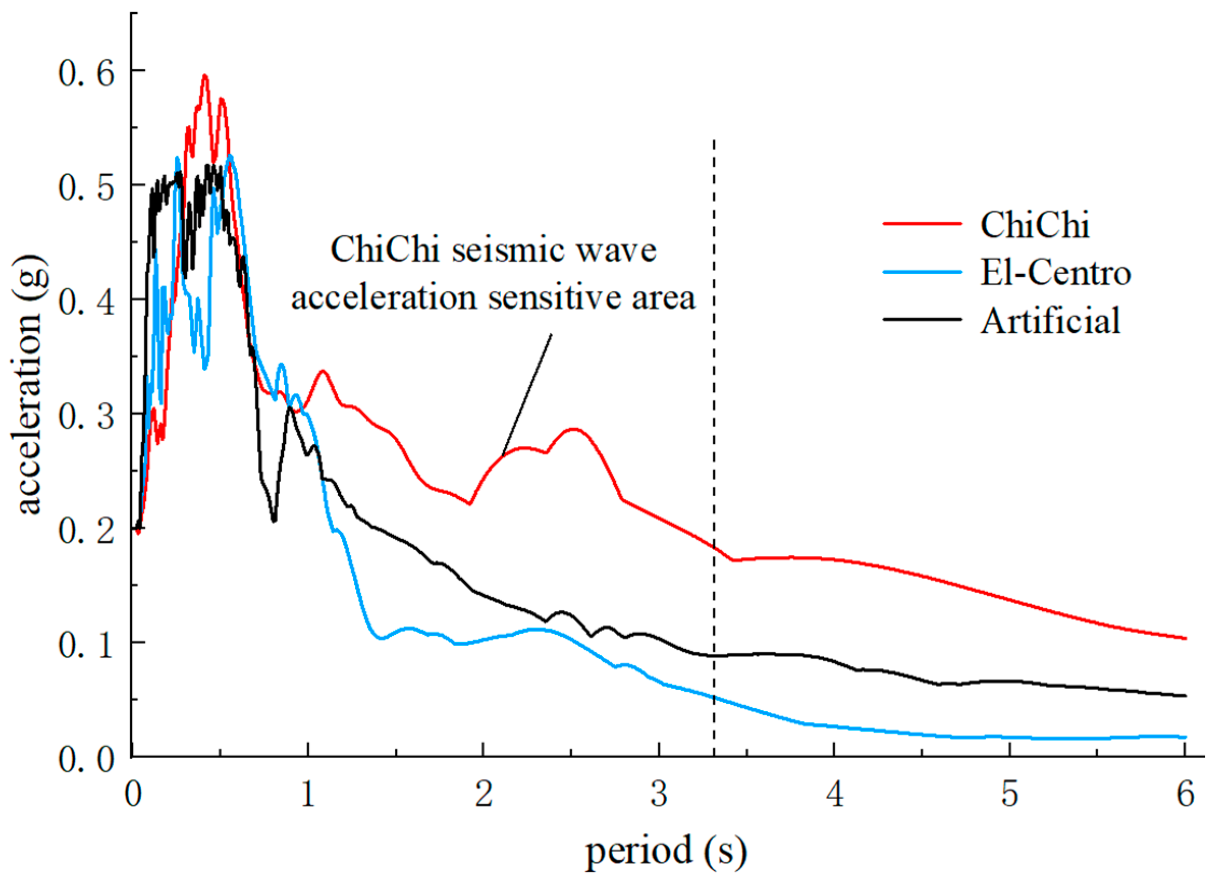
The acceleration response spectra of the three seismic waves are shown in Figure 9. The width of the acceleration-sensitive area of the El-Centro seismic wave and the artificial seismic wave is narrow, and their acceleration response spectra reach a peak in a short period and then decline rapidly. However, the acceleration-sensitive area of the Chi-Chi seismic wave with the characteristic of a velocity pulse is obviously wider, and the acceleration response spectra decrease relatively slowly.

5. Calculation Results and Analysis

5.1. The Response of Soil Acceleration

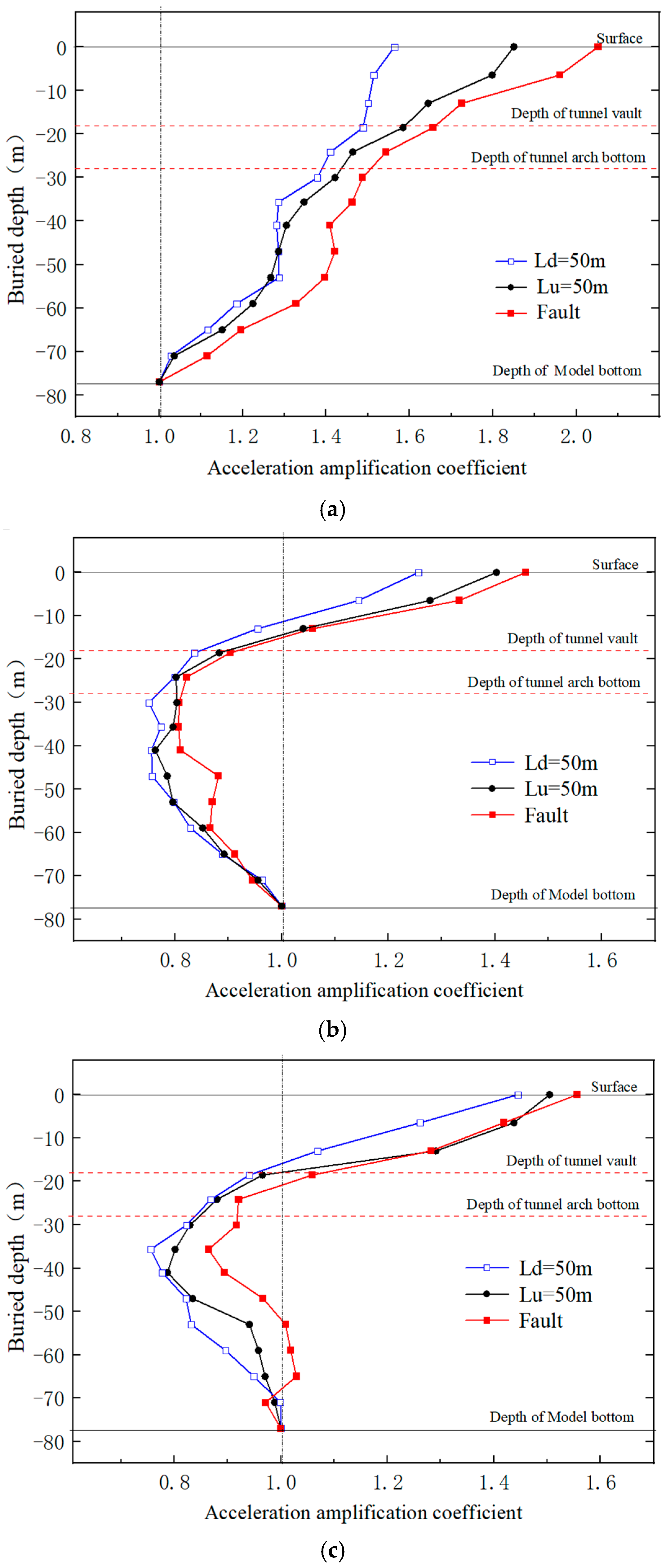
For convenience, Lu represents the distance from the measuring point of the hanging wall to the center of the fault, and Ld represents the distance from the measuring point of the footwall to the center of the fault. The peak soil accelerations were extracted along the buried depth direction at the position of the fault, and Lu = 50 m and Ld = 50 m, respectively. Their amplification coefficients (the ratio of the peak of acceleration at the measuring point to the peak of acceleration at the bottom of the model) are shown in Figure 10. In this section, the coefficients refer to the amplification coefficients of the peak soil accelerations.

The coefficients of the three seismic waves at different fields all show a field effect of fault > hanging wall > footwall, but the field effect is noticeable under the action of the Chi-Chi seismic wave.

The variation characteristics of the coefficients with different seismic waves along the direction of the burial depth were compared. The soil acceleration response of the El-Centro wave is similar to that of the artificial wave, and the coefficients of the El-Centro wave are slightly larger than the artificial wave in numerical terms. Under the action of the artificial wave and El-Centro wave, the coefficients decrease first from bottom to top and then increase, and only the coefficients less than a certain depth are larger than one. Under the action of the Chi-Chi wave, the coefficients continuously increase from the bottom up, and the coefficients from the bottom of the soil layer through the entire burial depth range are larger than one. The coefficients of the Chi-Chi wave are far higher than that of the El-Centro wave and the artificial wave in numerical terms.

The coefficients of different seismic waves according to the burial depth of the tunnel vault (−18 m) were compared. The coefficients of the Chi-Chi wave, artificial wave, and El-Centro wave in the fault are 1.66, 0.91, and 1.05, respectively; the coefficients of the hanging wall are 1.58, 0.85, and 0.95, respectively; and the coefficients of the footwall are 1.48, 0.83, and 0.94, respectively. Thus, the coefficient of the Chi-Chi wave is about 1.8 times that of the artificial wave and about 1.6 times that of the El-Centro wave.

5.2. The Response of Tunnel Acceleration

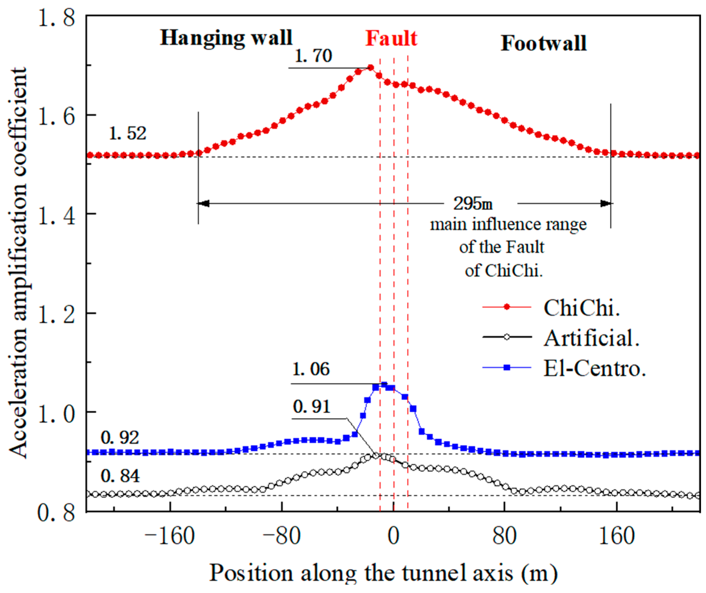
The tunnel is a long, linear structure, and there is a slight difference in the acceleration of each part of the tunnel under longitudinal seismic action. As shown in Figure 11, this paper analyzes the longitudinal distribution characteristics of the acceleration of the tunnel by taking the amplification coefficient of the peak acceleration of the tunnel vault as an example. In this section, the coefficients refer to the amplification coefficients of the peak vault acceleration.

The fault has a significant amplification effect on the response of tunnel acceleration. Similarly, the main range of influence of the fault on the tunnel’s longitudinal acceleration under the action of the Chi-Chi wave is more extensive than that of the El-Centro wave and the artificial wave.

Under the action of the different seismic waves, the maximum coefficients all appear in the fault zone and near the first slip surface. The maximum coefficients of the Chi-Chi wave, artificial wave, and El-Centro wave are 1.70, 0.91, and 1.06, respectively, and that of the Chi-Chi wave is about 1.8 times the artificial wave and 1.6 times the El-Centro wave. In the hanging wall and footwall areas far from the fault, the coefficients are more stable. The coefficients of the Chi-Chi wave, artificial wave, and El-Centro wave are about 1.52, 0.84, and 0.92, respectively, and the coefficients of the Chi-Chi wave are also about 1.8 times those of the artificial wave and about 1.6 times those of the El-Centro wave. In addition, the coefficients of the artificial wave are all less than one; the coefficients of the El-Centro wave are larger than one only near the fault; and the coefficients of the Chi-Chi wave are all larger than one.

In summary, for the metro tunnel crossing the fault, the response of soil acceleration and tunnel acceleration under the action of near-field seismic waves is significantly more potent than that under the far-field seismic waves.

5.3. The Response of Soil Pressure

Figure 12 shows the curves of peak soil pressure at the measuring points of the tunnel vault, hance, and arch bottom. The distribution characteristics of the peak soil pressure under the action of the three seismic waves are basically the same; the difference is only reflected in the numerical value of the peak soil pressure. The peak soil pressures of the El-Centro wave and that of the artificial wave are close to each other, while the peak soil pressure of the Chi-Chi wave is obviously larger than that of the El-Centro wave and the artificial wave. In particular, the peak soil pressure of the Chi-Chi wave is obviously larger at the fault slip surfaces, which indicates that the fault has a more significant influence on the distribution characteristics of soil pressure under near-field seismic action.

Taking the Chi-Chi wave as an example, the distribution characteristics of peak soil pressure along the tunnel axis were analyzed. As shown in Figure 12a,b, the curves of the vault and arch bottom of the tunnel located in the hanging wall and footwall sections are relatively straight, and the range of peak soil pressure is about 0.19 to 0.35 MPa. However, under the influence of the fault, the peak soil pressure of the tunnel located at slip surfaces increases significantly. The peak soil pressure at the first slip surface is most significant, and the most significant soil pressures of the vault and arch bottom at the first slip surface are 1.88 MPa and 1.46 MPa, respectively, which are much higher than the soil pressure in the hanging wall and footwall sections of the tunnel. The reason for this result is that soil activity near the fault is more intense under seismic action, and the soil dislocation caused by seismic action on the slip surfaces will directly act on the tunnel structure, resulting in the dynamic soil pressure of the tunnel at the slip surfaces being much larger than that at other locations.

As shown in Figure 12c, the curve of the tunnel hance is always relatively flat. The peak soil pressure does not change much, even at the slip surfaces. The numerical value of peak soil pressure ranges from 0.17 to 0.34 MPa. This indicates that the horizontal interaction between the soil and tunnel under longitudinal seismic action is less than the vertical interaction, resulting in the dynamic soil pressure of the horizontal lateral hance being correspondingly weaker than the dynamic soil pressure of the vertical vault and arch bottom.

5.4. The Response of Tunnel Longitudinal Internal Forces

5.4.1. Longitudinal Bending Moment

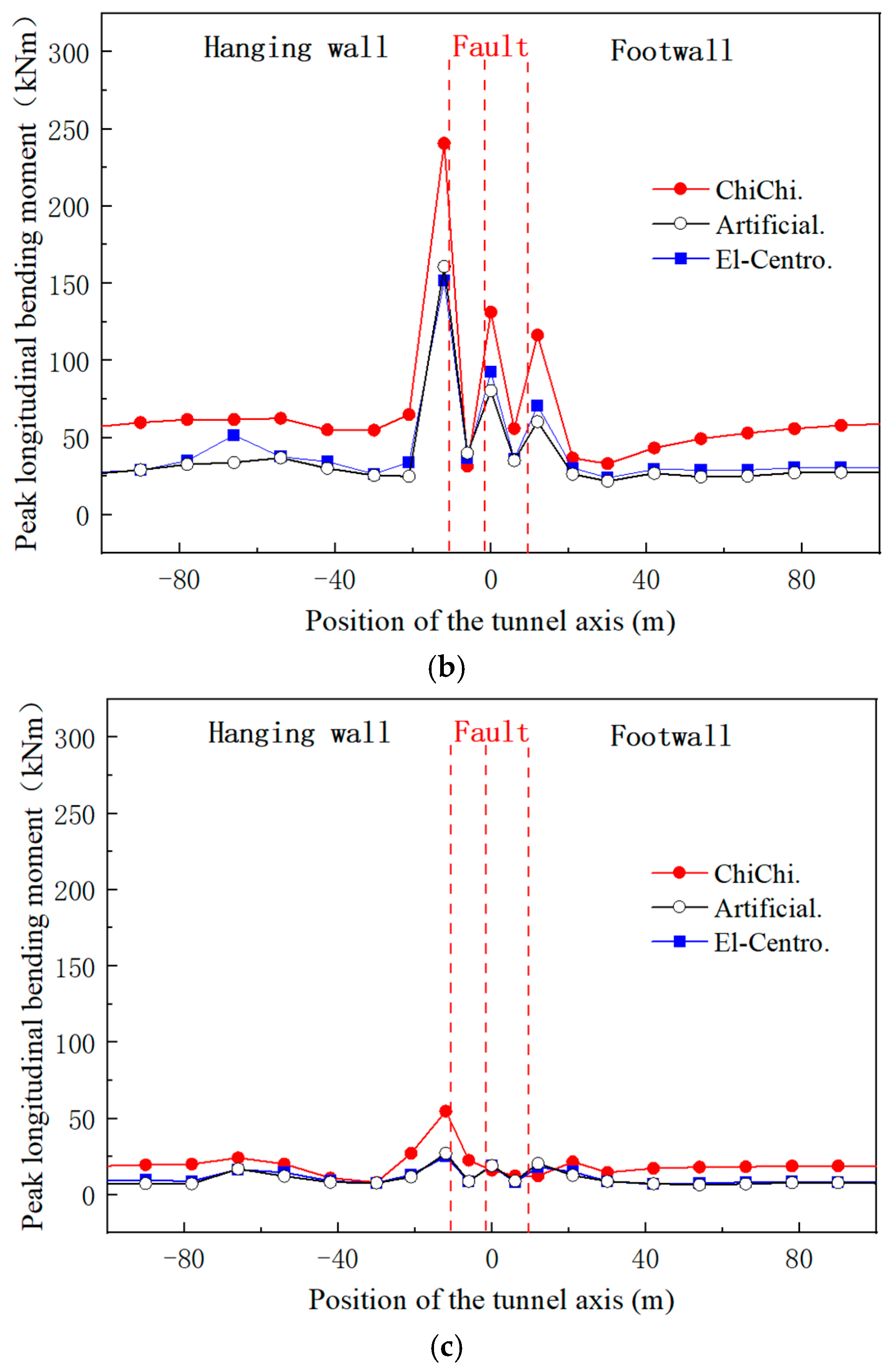
Figure 13 shows the curves of the peak longitudinal bending moment at the measuring points of the tunnel vault, hance, and arch bottom. The distribution characteristics of the peak longitudinal bending moment of different seismic waves are basically the same, and the difference is only reflected in the numerical value of the peak longitudinal bending moment. In numerical terms, the El-Centro wave and the artificial wave are close, while the Chi-Chi wave is obviously larger than the El-Centro wave and the artificial wave.

The distribution characteristics of the longitudinal bending moment along the tunnel axis are similar to the distribution characteristics of the dynamic soil pressure. In the hanging wall and footwall areas, the curves of the longitudinal bending moment remain relatively gentle. When affected by a fault, the longitudinal bending moments of the tunnel vault and arch bottom increase significantly at the position of the slip surfaces. The longitudinal bending moment of the tunnel hance also increases at the position of the first slip surface, but the increment in bending moment is smaller than that of the vault and arch bottom.

The maximum longitudinal bending moments of the vault, arch bottom, and hance all also appear at the position near the first slip surface, and they are 282, 240, and 55k Nm, respectively, under Chi-Chi seismic action. It is evident that the vault and the arch bottom are far larger than the hance.

5.4.2. Longitudinal Stress

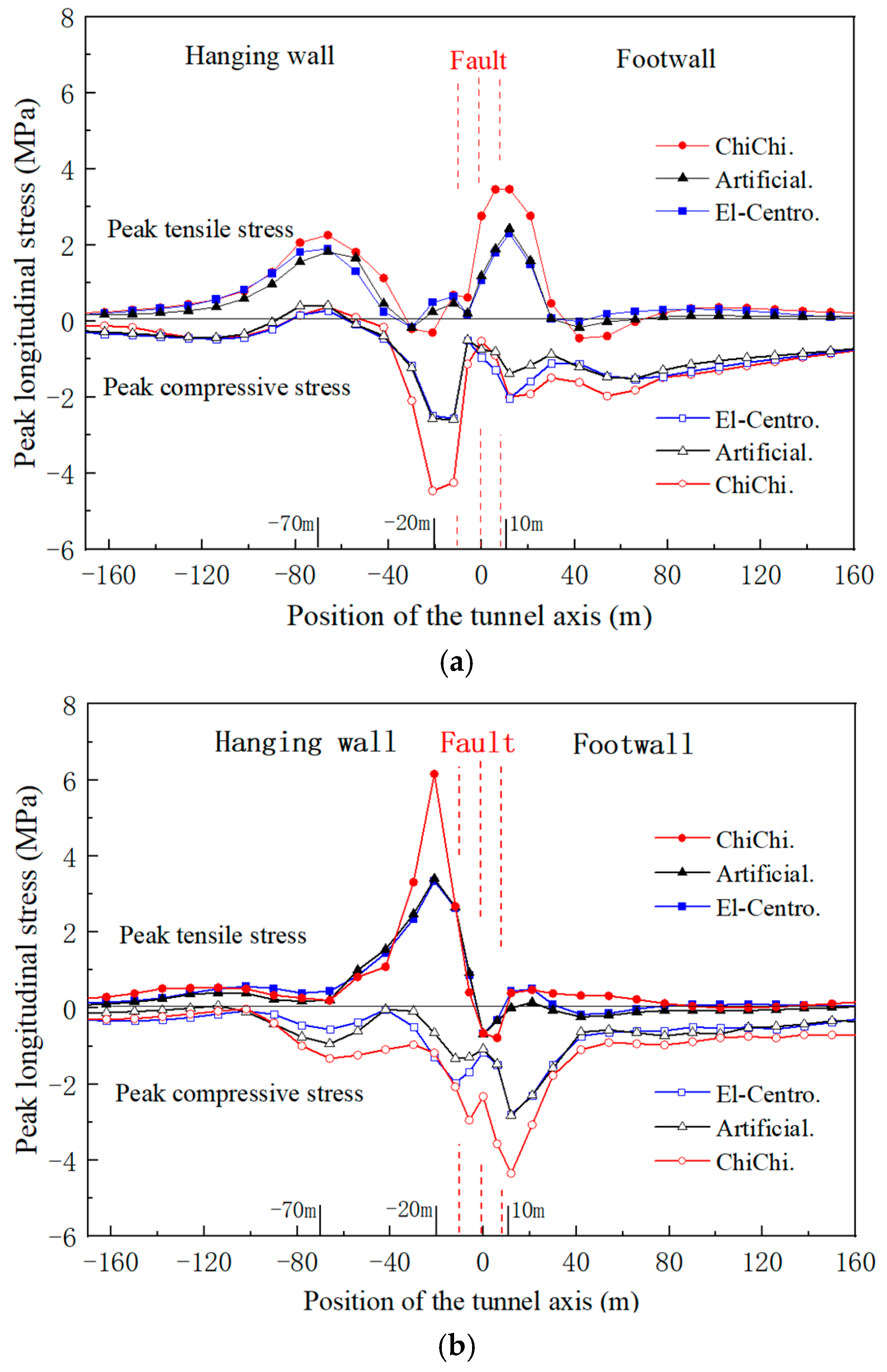
The maximum and minimum longitudinal stress of the tunnel vault and arch bottom measurement points are shown in Figure 14. Because the stress variation and stress magnitude of the tunnel hance are relatively gentle and small, analysis was not carried out. In Figure 14, positive stress indicates the peak tensile stress of the tunnel, and negative stress indicates the peak compressive stress of the tunnel.

The distribution characteristics of longitudinal stress at different seismic actions are also similar. The peak longitudinal stress of the Chi-Chi wave is generally larger than that of the El-Centro wave and the artificial wave in numerical terms, and that of the El-Centro wave and the artificial wave is closer. It appears that near-field seismic motion can cause larger internal forces in tunnel structures. Still, it has no significant impact on the distribution characteristics of internal forces along the tunnel axis.

Taking the Chi-Chi wave as an example, the distribution characteristics of tunnel longitudinal stress along the tunnel axial were analyzed. At the position Lu = 20 m, the peak compressive stress of the vault is much larger than the peak tensile stress, and the peak tensile stress of the arch bottom is much larger than the peak compressive stress, which indicates that the vault at this position is mainly compressed and the arch bottom is mainly tensed during the dynamic process. Thus, the tunnel has a deformation trend of bending downward. Near the position Lu = 70 m and Ld = 10 m, the peak tensile stress of the vault is far larger than the peak compressive stress, while the peak compressive stress of the arch bottom is far larger than the peak tensile stress. This indicates that the vault at these positions is mainly tensed, the arch bottom is mainly compressed during the dynamic process, and the tunnel has a deformation trend of bending upward.

The concrete material of the tunnel lining is more vulnerable to tensile damage, so special attention should be paid to the position of the tunnel structure with sizeable tensile stress. Under seismic action, the maximum tensile stress of the tunnel appears at the position of the arch bottom of the hanging wall near the first slip surface. The peak tensile stress at this position under Chi-Chi seismic action reaches 6.16 MPa, which is far higher than the design value of the axial tensile strength of C35 concrete material (1.57 MPa). In addition, the sizeable tensile stress also appeared at the vault near the positions Lu = 70 m and Ld = 10 m, and the peak tensile stress at these positions under Chi-Chi seismic action reached 2.26 and 3.46 MPa, respectively.

6. Discussion and Conclusions

This paper, using numerical simulation, studies the longitudinal seismic response of a metro tunnel orthogonally crossing a multi-slip surface fault. By analyzing the dynamic response such as acceleration, dynamic soil pressure, and longitudinal internal force, the following conclusions are drawn:

(1)

Compared with a far-field seismic wave, such as an artificial seismic wave and El-Centro seismic wave, the Chi-Chi seismic wave—a near-field seismic wave with velocity pulse—has larger PGV, PGD, and PGV/PGA, and its acceleration response spectrum has a wider acceleration-sensitive area.

(2)

Under seismic action, the soil acceleration of the fault field is larger than the hanging wall, and that of the hanging wall is larger than the footwall. The soil acceleration at different fields shows a noticeable “hanging wall field effect”, and the field effect is particularly noticeable under near-field seismic action.

(3)

The fault has a significant amplification influence on the tunnel acceleration response, and the range of influence of the fault under near-field seismic action is significantly larger than that under far-field seismic action. The maximum acceleration of the tunnel appears near the first slip surface. Overall, the acceleration response of both the soil and tunnel under near-field seismic action is much larger than that under far-field seismic actions.

(4)

Under the influence of the fault, the soil pressure and longitudinal bending moment near the fault slip surfaces increase significantly. The maximum soil pressure and the maximum longitudinal bending moment of the tunnel appear at the vault of the first slip surface. The maximum longitudinal stress appears at the arch bottom of the first slip surface. There is no significant difference in the distribution characteristics of the peak soil pressure and the peak internal force of the tunnel along the tunnel axis caused by different seismic actions. However, in numerical terms, the peak soil pressure and peak internal force of the tunnel under near-field seismic action are obviously larger than those under far-field seismic action.

To summarize, the longitudinal seismic response of the metro tunnel orthogonally crossing a multi-slip surfaces fault under near-field seismic action is significantly more potent than that under far-field seismic action. The tunnel is more susceptible to damage at the position of the slip surfaces under seismic action, especially near the slip surface between the hanging wall and the fault.

The above research results have reference values for the seismic response and seismic design of tunnels crossing a fault. However, there are still many shortcomings in this study due to the limited abilities of the authors. This paper explores this research topic only using theoretical numerical methods, and it is necessary to conduct shaking table experiments on metro tunnels crossing multi-slip surface faults. Future research direction should pay attention to the following key issues:

(1)

In the dynamic analysis of the Soil–Fault–Tunnel model, the model’s boundary is extremely critical and directly affects the reliability of the results. It is still necessary to optimize the artificial boundary of the model.

(2)

Research should consider more practical operating conditions, such as different tunnel intersection angles, fault dip angles, and fault widths.