

Developing Nomographs for the Unit Weight of Soils


Abstract
:1. Introduction
2. Methodology
2.1. Data Collection and Cleansing
2.2. Data Cleansing and Addressing Uncertainty
2.3. Modeling
2.4. Addressing Uncertainty
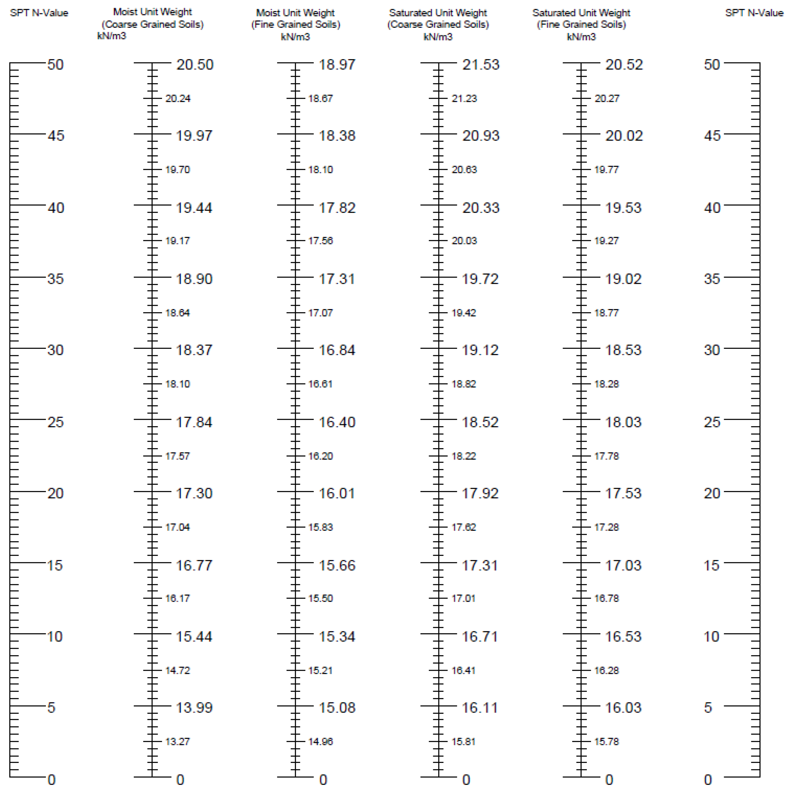
2.5. Nomographs
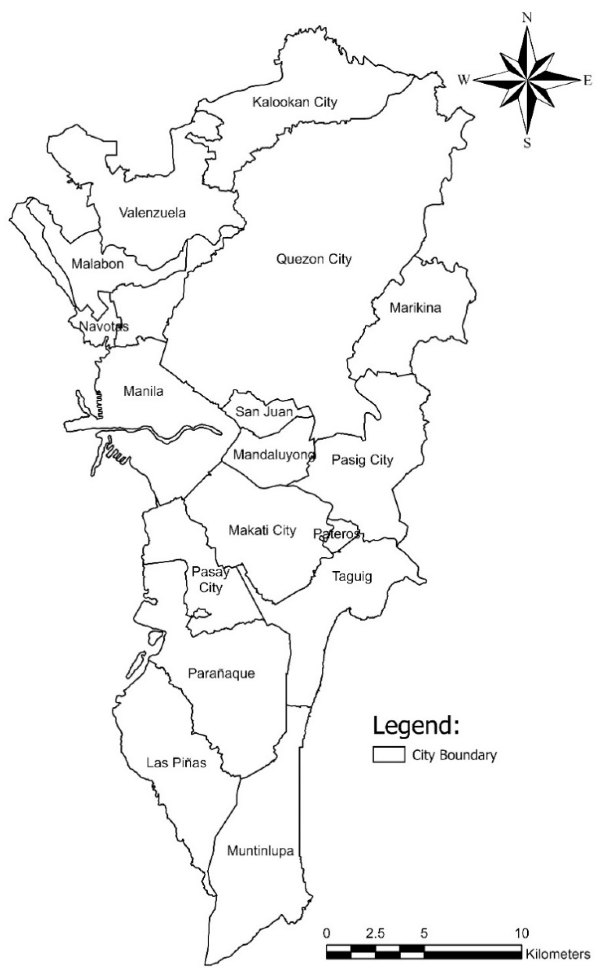
2.6. Case Study
3. Results and Discussion
3.1. Data Collected
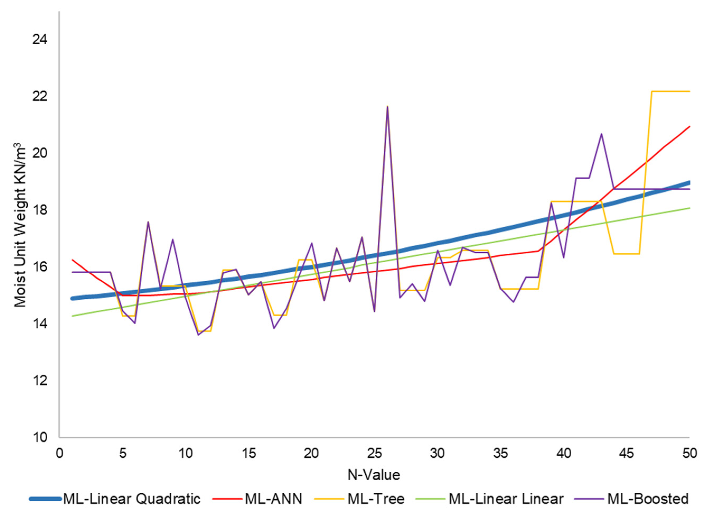
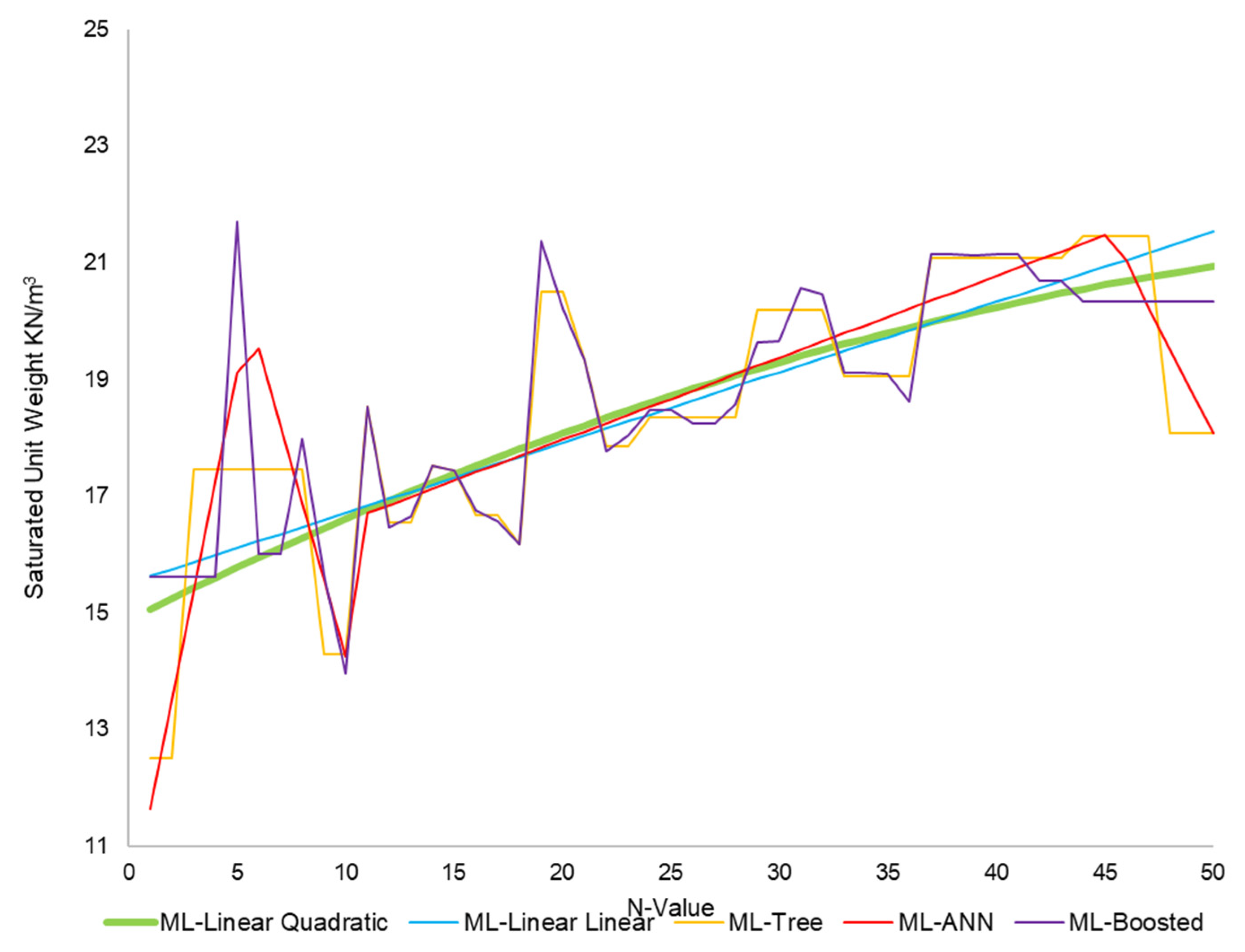
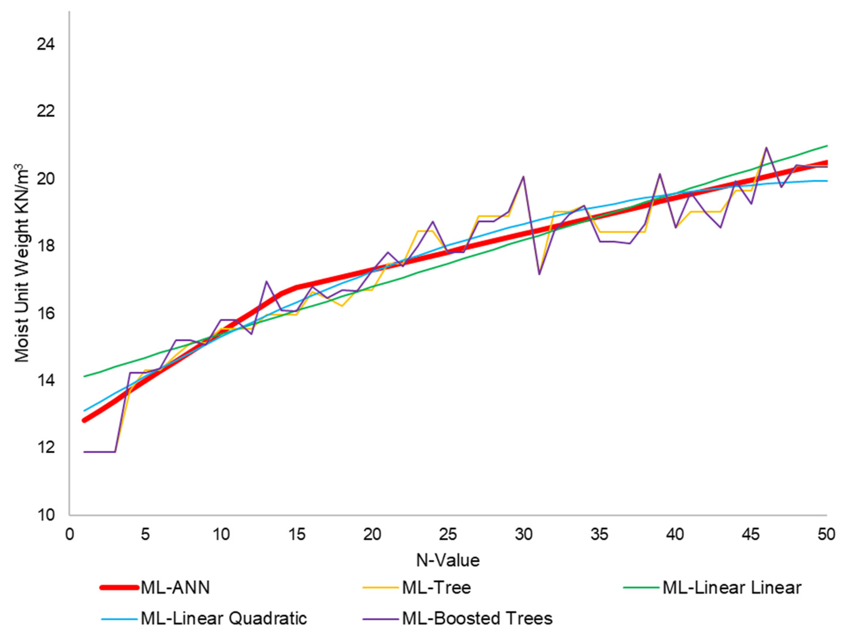
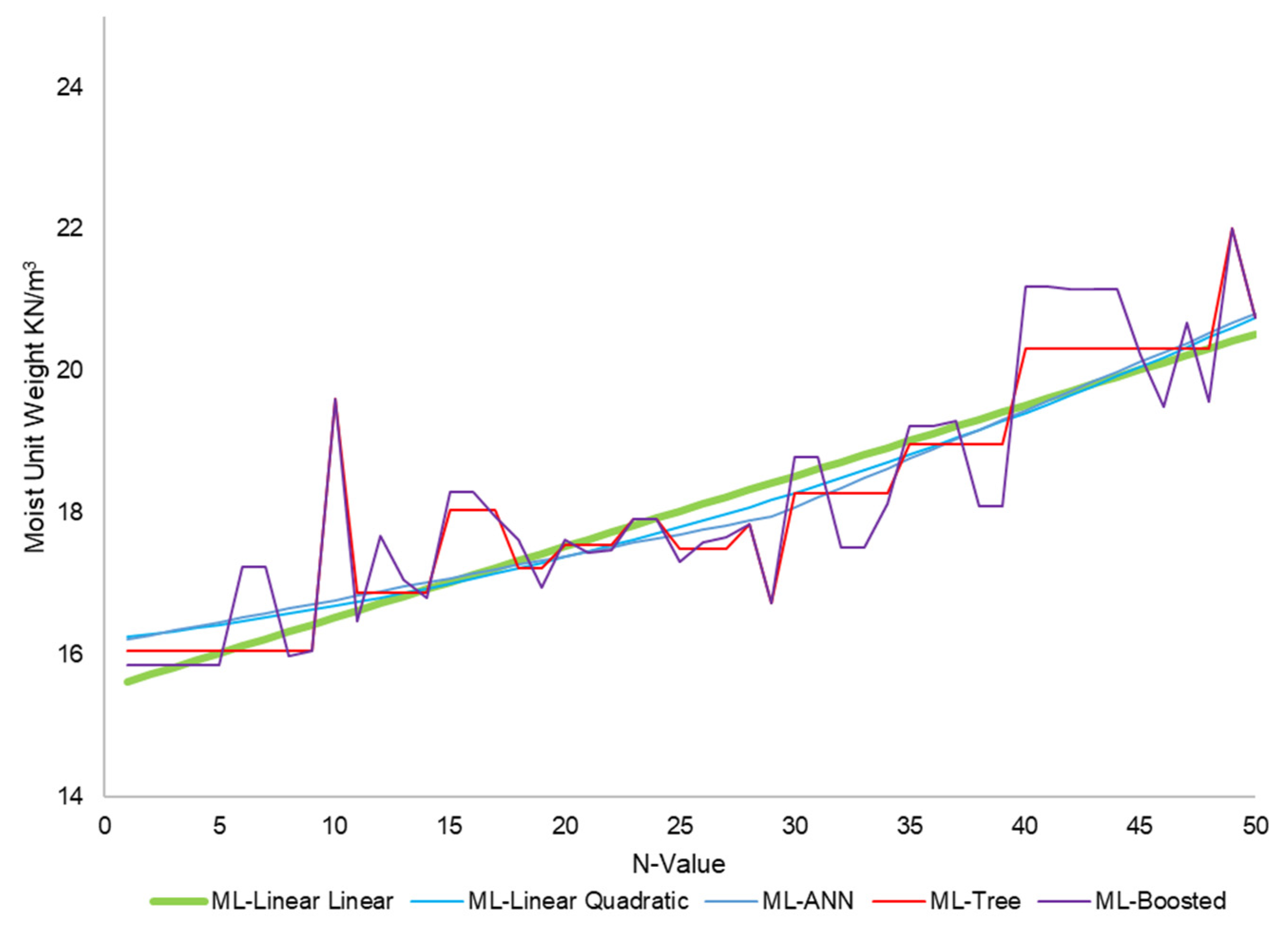
3.2. Models
3.3. Uncertainty Analysis
3.4. Nomographs
3.5. Deploying the Generated Nomograph to Metro Manila, Philippines
3.6. Further Validation
4. Conclusions and Recommendations
Author Contributions
Funding
Data Availability Statement
Acknowledgments
Conflicts of Interest
References
- Peck, R.; Hanson, W.; Thornburn, T. Foundation Engineering, 2nd ed.; John Wiley & Sons: Hoboken, NJ, USA, 1974; Volume 2. [Google Scholar]
- Ameratunga, J.; Sivakugan, N.; Das, B.M. Correlations of Soil and Rock Properties in Geotechnical Engineering; Springer: Berlin/Heidelberg, Germany, 2016. [Google Scholar]
- Terzaghi, K.; Peck, R.; Mesr, G. Soil Mechanics in Engineering Practice; John Wiley & Sons, Inc.: Hoboken, NJ, USA, 1996. [Google Scholar]
- Puri, N.; Prasad, H.D.; Jain, A. Prediction of Geotechnical Parameters Using Machine Learning Techniques. Procedia Comput. Sci. 2018, 125, 509–517. [Google Scholar] [CrossRef]
- Pynomo. Introduction—pyNomo Documentation 0.3.2.1 Documentation. Available online: http://pynomo.org/wiki/index.php/Software_documentation (accessed on 1 July 2022).
- Esmail, E.L. Nomographs for the synthesis of epicyclic-type automatic transmissions. Meccanica 2013, 48, 2037–2049. [Google Scholar] [CrossRef]
- McMillen, E.L. A Versatile Nomograph for Chemical Engineering Calculations. Ind. Eng. Chem. 1938, 30, 71–79. [Google Scholar] [CrossRef]
- Levens, A. Nomography; John Wiley & Sons, Inc.: Hoboken, NJ, USA, 1948. [Google Scholar]
- Glasser, L.; Doerfler, R. A brief introduction to nomography: Graphical representation of mathematical relationships. Int. J. Math. Educ. Sci. Technol. 2018, 50, 1273–1284. [Google Scholar] [CrossRef]
- Douglas, J.; Danciu, L. Nomogram to help explain probabilistic seismic hazard. J. Seismol. 2020, 24, 221–228. [Google Scholar] [CrossRef]
- Coker, A.K. Cost estimation and economic evaluation. Ludwig’s Appl. Process Des. Chem. Petrochem. Plants 2017, 1, 69–102. [Google Scholar]
- Skibniewski, M.J.; Nof, S.Y. A framework for programmable and flexible construction systems. Robot. Auton. Syst. 1989, 5, 135–150. [Google Scholar] [CrossRef]
- Zhao, Z.; Guan, X.; Xiao, F.; Xie, Z.; Xia, P.; Zhou, Q. Applications of asphalt concrete overlay on Portland cement concrete pavement. Constr. Build. Mater. 2020, 264, 120045. [Google Scholar] [CrossRef]
- Mahpour, A.; El-Diraby, T. Incorporating Climate Change in Pavement Maintenance Policies: Application to Temperature Rise in the Isfahan County, Iran. Sustain. Cities Soc. 2021, 71, 102960. [Google Scholar] [CrossRef]
- Mandare, A.B.; Ambast, S.K.; Tyagi, N.K.; Singh, J. On-farm water management in saline groundwater area under scarce canal water supply condition in the Northwest India. Agric. Water Manag. 2008, 95, 516–526. [Google Scholar] [CrossRef]
- Moatar, F.; Person, G.; Meybeck, M.; Coynel, A.; Etcheber, H.; Crouzet, P. The influence of contrasting suspended particulate matter transport regimes on the bias and precision of flux estimates. Sci. Total Environ. 2006, 370, 515–531. [Google Scholar] [CrossRef] [PubMed]
- Barker, G. Pipe sizing and pressure drop calculations. In The Engineer’s Guide to Plant Layout and Piping Design for the Oil and Gas Industries; Elsevier: Amsterdam, The Netherlands, 2018; pp. 411–472. [Google Scholar]
- Chien, S.F. Laminar flow pressure loss and flow pattern transition of Bingham plastics in pipes and annuli. Int. J. Rock Mech. Min. Sci. 1970, 7, 339–356. [Google Scholar] [CrossRef]
- Gamage, S.H.P.W.; Hewa, G.A.; Beecham, S. Modelling hydrological losses for varying rainfall and moisture conditions in South Australian catchments. J. Hydrol. Reg. Stud. 2015, 4, 1–21. [Google Scholar] [CrossRef]
- Haan, C.T.; Barfield, B.J.; Hayes, J.C. Hydraulics of Structures. In Design Hydrology and Sedimentology for Small Catchment; Elsevier: Amsterdam, The Netherlands, 1994; pp. 144–181. [Google Scholar]
- Srivastava, J.B.; Gupta, A.K.; Khanna, S.K. Modelling of Highway Traffic Pollution. IFAC Proc. Vol. 1994, 27, 889–891. [Google Scholar] [CrossRef]
- Burke, C.M.; Scott, D.M. The space race: A framework to evaluate the potential travel-time impacts of reallocating road space to bicycle facilities. J. Transp. Geogr. 2016, 56, 110–119. [Google Scholar] [CrossRef]
- Fricke, L.B. Traffic management and collision investigation. Accid. Anal. Prev. 1982, 14, 486–487. [Google Scholar] [CrossRef]
- Martinelli, P.; Colombo, M.; Ravasini, S.; Belletti, B. Application of an analytical method for the design for robustness of RC flat slab buildings. Eng. Struct. 2022, 258, 114117. [Google Scholar] [CrossRef]
- Minami, F.; Ohata, M.; Shimanuki, H.; Handa, T.; Igi, S.; Kurihara, M.; Kawabata, T.; Yamashita, Y.; Tagawa, T.; Hagihara, Y. Method of constraint loss correction of CTOD fracture toughness for fracture assessment of steel components. Eng. Fract. Mech. 2006, 73, 1996–2020. [Google Scholar] [CrossRef]
- Chala, A.T.; Ray, R.P. Machine Learning Techniques for Soil Characterization Using Cone Penetration Test Data. Appl. Sci. 2023, 13, 8286. [Google Scholar] [CrossRef]
- Daghistani, F.; Abuel-Naga, H. Evaluating the Influence of Sand Particle Morphology on Shear Strength: A Comparison of Experimental and Machine Learning Approaches. Appl. Sci. 2023, 13, 8160. [Google Scholar] [CrossRef]
- Cheng, H.; Zhang, H.; Liu, Z.; Wu, Y. Prediction of Undrained Bearing Capacity of Skirted Foundation in Spatially Variable Soils Based on Convolutional Neural Network. Appl. Sci. 2023, 13, 6624. [Google Scholar] [CrossRef]
- Chala, A.T.; Ray, R. Assessing the Performance of Machine Learning Algorithms for Soil Classification Using Cone Penetration Test Data. Appl. Sci. 2023, 13, 5758. [Google Scholar] [CrossRef]
- Lee, S.; Kang, J.; Kim, J. Prediction Modeling of Ground Subsidence Risk Based on Machine Learning Using the Attribute Information of Underground Utilities in Urban Areas in Korea. Appl. Sci. 2023, 13, 5566. [Google Scholar] [CrossRef]
- Dufour, J.C.; Mancini, J.; Fieschi, M. Searching for evidence-based data. J. Chir. 2009, 146, 355–367. [Google Scholar] [CrossRef] [PubMed]
- Safadi, M.; Ma, J.; Wickramasuriya, R.; Daly, D.; Perez, P.; Kokogiannakis, G. Mapping for the Future: Business Intelligence Tool to Map Regional Housing Stock. Procedia Eng. 2017, 180, 1684–1694. [Google Scholar] [CrossRef]
- Bowles, J.E. Foundation Analysis and Design. In Civil Engineering Materials; The McGraw-Hill Companies, Inc.: New York, NY, USA, 1997. [Google Scholar]
- Rahman, M. Foundation Design using Standard Penetration Test (SPT) N-value. Researchgate 2019, 5, 1–39. [Google Scholar]


| SPT N-Value | Unit Weight (kN/m3) |
|---|---|
| 0–4 | 11.00–15.71 |
| 4–10 | 14.14–18.07 |
| 10–30 | 17.28–20.42 |
| 30–50 | 17.28–22.00 |
| >50 | 20.42–23.56 |
| Soil Layer Location | Reference Parameter | Correlating Parameter |
|---|---|---|
| Above Groundwater Table | SPT N-Value | Moist unit weight of coarse-grained soils |
| Moist unit weight of fine-grained soils | ||
| Below Groundwater Table | Saturated unit weight of coarse-grained soils | |
| Saturated unit weight of fine-grained soils |
| Coefficient of Determination (R2) | Interpretation |
|---|---|
| >0.70 | Very Strong Positive Relationship |
| 0.40–0.69 | Strong Positive Relationship |
| 0.30–0.39 | Moderate Positive Relationship |
| 0.20–0.29 | Weak Positive Relationship |
| 0.01–0.19 | Negligible Relationship |
| 0 | No Relationship |
| Independent Scale | Dependent Scale |
|---|---|
| SPT N-Value | Moist unit weight (coarse-grained soils) |
| Moist unit weight (fine-grained soils) | |
| Saturated unit weight (coarse-grained soils) | |
| Saturated unit weight (fine-grained soils) |
| No. of Data | Description |
|---|---|
| 158 | Moist-coarse |
| 120 | Moist-fine |
| 94 | Saturated-coarse |
| 86 | Saturated-fine |
| Variable | Mean | Conf. | Conf. | Min | Max | Var | Std. Dev. | Conf. SD | Conf. SD | Coef. Var. | Skewness |
|---|---|---|---|---|---|---|---|---|---|---|---|
| SPT N-Value | 28.11 | 27.96 | 28.25 | 1.00 | 50.00 | 382.90 | 19.57 | 19.47 | 19.67 | 69.62 | −0.04 |
| Unit Weight | 17.95 | 17.93 | 17.96 | 13.10 | 20.93 | 5.37 | 2.31674 | 2.30 | 2.33 | 12.91 | 0.00 |
Disclaimer/Publisher’s Note: The statements, opinions and data contained in all publications are solely those of the individual author(s) and contributor(s) and not of MDPI and/or the editor(s). MDPI and/or the editor(s) disclaim responsibility for any injury to people or property resulting from any ideas, methods, instructions or products referred to in the content. |
© 2023 by the authors. Licensee MDPI, Basel, Switzerland. This article is an open access article distributed under the terms and conditions of the Creative Commons Attribution (CC BY) license (https://creativecommons.org/licenses/by/4.0/).
Share and Cite
Dungca, J.; Galupino, J. Developing Nomographs for the Unit Weight of Soils. Buildings 2023, 13, 2315. https://doi.org/10.3390/buildings13092315
Dungca J, Galupino J. Developing Nomographs for the Unit Weight of Soils. Buildings. 2023; 13(9):2315. https://doi.org/10.3390/buildings13092315
Chicago/Turabian StyleDungca, Jonathan, and Joenel Galupino. 2023. "Developing Nomographs for the Unit Weight of Soils" Buildings 13, no. 9: 2315. https://doi.org/10.3390/buildings13092315
APA StyleDungca, J., & Galupino, J. (2023). Developing Nomographs for the Unit Weight of Soils. Buildings, 13(9), 2315. https://doi.org/10.3390/buildings13092315