Finite Element Analysis of Curved Beam Elements Employing Trigonometric Displacement Distribution Patterns

Abstract

A finite element analysis (FEA) model was developed for Euler and Timoshenko curved beam elements by incorporating trigonometric displacement distribution patterns. Local polar coordinate stiffness matrices were derived based on force-displacement relations and static equilibrium conditions. By employing the kinetic energy theorem and triangular displacement functions, an expression for the consistent mass matrix of a curved beam element was obtained. A coordinate transformation matrix for the curved beam element was established by relating the local polar coordinate system to the global polar coordinate system. Calculation programs were implemented in the Fortran language to evaluate the static–dynamic performance and natural frequency characteristics of curved beam bridges. The obtained results were then compared with those obtained using ANSYS solid models and “replace curve with straight” beam element models. The comparison demonstrated a strong agreement between the results of the Euler and Timoshenko curved beam element models and those of the ANSYS solid models. However, discrepancies were observed when comparing with the results of the “replace curve with straight” beam element model, particularly in terms of lateral static displacement. This discrepancy suggests that the characteristic matrix derived in this study accurately represents the stiffness and mass distribution of the curved beam, making it suitable for mechanical performance analysis of curved beam bridges. It should be noted that the “replace curve with straight” method overlooks the initial curvature and the bending–torsion coupling effects of a curved beam, resulting in calculation deviations. On the other hand, the use of curved beam elements in numerical analysis provides a simple and practical approach, which facilitates further research in areas such as vehicle–bridge coupling vibrations and seismic analysis of curved beam bridges.

1. Introduction

With the advancement of modern construction techniques and the increasing demand for aesthetic appeal in structural design, curved beams have found extensive utilization within bridge structures. Given the intricacies of load distribution and complex stress patterns in curved beams, structural analysis presents significant challenges. Currently, the prevalent approach involves approximating curved beams by using straight beams, referred to as the “straight in lieu of curved” method. However, this approach disregards the bending–torsion coupling effects inherent in curved beams. Moreover, substituting straight beams for curved ones fails to capture these coupling effects, leading to issues of a slow convergence during the solution process and substantial computational inaccuracies. Especially when dealing with curved beams of small radii, approximation using straight beams to simulate the behavior of curved beams proves inadequate for meeting the accuracy demanded by real-world engineering applications in curved beam bridges. Thus, it becomes imperative to establish specialized curved beam elements that accurately reflect the mechanical characteristics of curved beams, enabling a more precise simulation of curved beam bridge behavior [1,2,3,4,5,6].

In recent years, several researchers have conducted studies on the finite element analysis of curved beam elements [7,8,9,10,11]. Guo Weitong et al. [12] derived control equations for the axial and radial displacements of curved beams by analyzing equilibrium equations, geometric equations, and physical equations. They obtained analytical solutions and expressed the stiffness equilibrium equations in matrix form to derive the stiffness matrix and equivalent nodal force vector of the curved beam element. The accuracy and efficiency of the curved beam element were verified through numerical examples.

Nadi A et al. [13] proposed a finite element method for analyzing in-plane vibrations of Timoshenko curved beams. They derived the stiffness matrix and mass matrix of a curved beam element, considering shear deformation and rotational inertia, based on the force–displacement relationship and kinetic energy theorem. They also investigated the effect of tuned mass dampers on the vibration response of the curved beam.

Chen Jinhua [14] established out-of-plane and in-plane homogeneous equilibrium vibration equations to address phenomena such as membrane force locking and shear force locking in curved beam elements. They obtained triangular displacement field functions that satisfy the rigid body displacement conditions through numerical calculations. A stiffness matrix and consistent mass matrix of the curved beam element that satisfied the boundary conditions were derived. The results showed that the element had a good calculation accuracy.

Li Xingzhao et al. [15] used the Euler–Bernoulli beam model to establish a free vibration differential equation for circular curved beams. They derived a decoupling solution method for differential equations through theoretical derivation and verified the correctness of the theoretical method using the finite element method.

The preceding body of literature underscores the inclination of prior investigations towards the utilization of differential equation solutions or the scrutiny of hyperstatic frameworks for the execution of a finite element analysis pertaining to curved beams. Nevertheless, scholarly inquiries centered upon the examination of the in-plane or out-of-plane oscillations exhibited by curved beams through the employment of dedicated curved beam elements are notably scarce. These methodologies, due to their inherent intricacies and complexities, have not garnered widespread acceptance within the realm of pragmatic implementations.

Within the framework of finite element theory, it is customary to define suitable shape functions for elements and deduce element characteristic matrices that account for shear deformation by employing the principle of minimum potential energy or the virtual work principle. The selection of appropriate shape functions is a pivotal aspect of finite element analysis. When utilizing polynomial interpolation functions as displacement distribution patterns for curved beam elements, the presence of an initial curvature introduces a “bending–torsion coupling” effect. Unlike straight beam elements, it becomes challenging to incorporate shear deformation into curved beam elements through equilibrium equations at the element level. This intricacy contributes to the heightened complexity of finite element analysis of curved beam elements.

For beams with large span-to-depth ratios, the contribution of shear deformation to deflection cannot be overlooked. In such cases, applying curved beam elements that do not account for shear effects imposes limitations when employed in engineering practice. Consequently, there arises a need to explore an alternative displacement distribution pattern that considers shear deformation and deviates from polynomial forms. This would enable the establishment of a finite element analysis model for curved beam elements that accurately incorporates shear effects.

Due to the potential limitations of conventional linear displacement distribution patterns in describing structural deformations, especially for structures with curved geometries, the introduction of triangular displacement distribution patterns offers a more precise approximation of complex curved deformations, thereby enhancing the accuracy of the analysis model. Therefore, this paper presents a novel approach based on finite element analysis theory. It introduces a new methodology that incorporates triangular function displacement distribution patterns satisfying the equilibrium differential equations of curved beams. The methodology derives characteristic matrices for two types of spatial curved beam elements: Euler and Timoshenko elements, which are decoupled for out-of-plane and in-plane vibrations. It further establishes a coordinate transformation matrix between local polar coordinates and global polar coordinates. The correctness of this methodology is verified through numerical examples, thus providing a valuable reference for finite element analysis of curved beam elements.

2. Displacement Distribution Pattern of Triangular Function for Curved Beam Element

2.1. Basic Assumptions

During the finite element analysis of curved beam elements, several assumptions are generally made to ensure accuracy and efficiency. First, linear elasticity is assumed for the material. Second, the dimensions of the curved beam section are assumed to be small in comparison to the span and radius of the curvature. Third, transverse shear deformation and rotational inertia effects are taken into account, while cross-sectional distortions and shear lag effects are neglected. Finally, the curved beam element is treated as a circular arc element with a constant radius of curvature for each individual element [16].

Figure 1 illustrates the definitions of the local coordinate system, global coordinate system, node displacements, and internal forces for both out-of-plane and in-plane analysis of a spatial curved beam element. The global coordinate system for a curved beam element is represented as XYZ, while the local coordinate system for the element is denoted as xyz(θ). It is important to note that the directions of the coordinate systems are based on the right-hand rule. Furthermore, R denotes the radius of curvature, l represents the length of the curved beam element, θ signifies the angle between any point within the element and the negative x-axis, θ₁ and θ₂ represent the angles between the two nodes of the element, and points ① and ② are positioned at the extremities of the circular arc, serving as its terminal points. These definitions provide a comprehensive understanding of the coordinate systems and parameters involved in analyzing the spatial curved beam element.

A spatial curved beam element is designed with three degrees of freedom in-plane for each node, comprising the axial displacement u_x, radial displacement u_y, and rotational displacement φ_z. Furthermore, three degrees of freedom out-of-plane are provided at each node, including the vertical displacement u_z, rotational displacement φ_y, and torsional angle φ_x. The nodal degree of freedom vector for the spatial curved beam element encompasses twelve degrees of freedom in total, which can be expressed as follows:

$${\delta }^e={[\begin{array}{cccccccccccc}{u}_{x1}& u_{y1}& u_{z1}& {\phi }_{x1}& {\phi }_{y1}& {\phi }_{z1}& u_{x2}& u_{y2}& u_{z2}& {\phi }_{x2}& {\phi }_{y2}& {\phi }_{z2}\end{array}]}^T$$

(1)

In this equation, subscripts 1 and 2 refer to the identification of the two nodes of the element. u_x1(2), u_y1(2), and u_z1(2) represent the linear displacements along the local coordinate axes. Meanwhile, φ_x1(2), φ_y1(2), and φ_z1(2) depict the rotational displacements about the local coordinate axes.

The nodal loads associated with the displacements of the nodes for the spatial curved beam element are given as follows:

$$F^e={\left[\begin{array}{c}\begin{array}{cccccccccccc}{F}_{x1}& F_{y1}& F_{z1}& M_{x1}& M_{y1}& M_{z1}& F_{x2}& F_{y2}& F_{z2}& M_{x2}& M_{y2}& M_{z2}\end{array}\end{array}\right]}^T$$

(2)

In this equation, F_x1(2), F_y1(2), and F_z1(2) are the axial forces and shear forces along the local coordinate axis, while M_x1(2), M_y1(2), and M_z1(2) are the bending and torsional moments around the local coordinate axis. Specifically, the bending moment (around the y-axis) is positive when the lower side of the beam is under tension, and the bending moment (around the z-axis) is positive when the outer side of the beam is under tension. The torsion moment is positive when it points from the inside to the outside of the beam, and the axial force is positive when the beam is under tension.

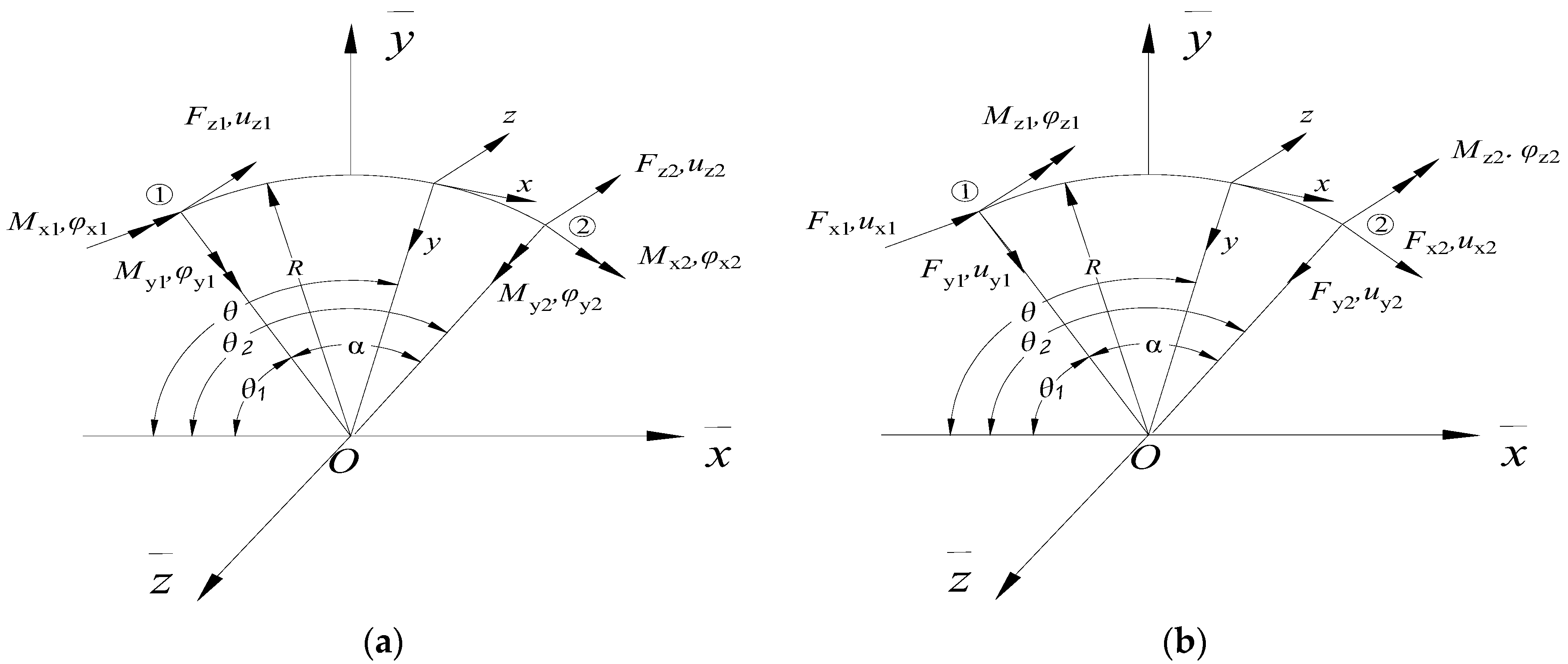
2.2. Displacement Shape Functions of a Curved Beam Element

Before determining the displacement shape function for the curved beam element, it is necessary to combine the differential equation for the curved beam and derive an expression for the displacement function that satisfies the spatial vibration equation through numerical methods [17]. Based on this, the displacement shape functions for the out-of-plane and in-plane displacements of the curved beam element in the local coordinate system can be derived using the internal force–displacement relationship and the static equilibrium equation [18,19]. For the infinitesimal curved beam element shown in Figure 1, assuming the cross-section remains constant along the entire length of the beam and is in a state of static equilibrium, the expressions for the linear displacement and angular displacement along the local coordinate axes can be given as:

$$\{\begin{array}{l}{u}_{out}=H_{out}{B}_{out}\\ u_{in}=H_{in}{B}_{in}\end{array}$$

(3)

In this equation, u_out and u_in represent the degrees of freedom for the out-of-plane and in-plane displacements of the curved beam element, respectively.

$$u_{out}=\left\{u_z(\theta ),{\phi }_x(\theta ),{\phi }_y(\theta )\right\};$$

$$u_{in}=\left\{u_x(\theta ),u_y(\theta ),{\phi }_z(\theta )\right\}$$

(4)

$$B_{out}={\left\{B_1,B_2,B_3,B_4,B_5,B_6\right\}}^T; B_{in}={\left\{B_7,B_8,B_9,B_{10},B_{11},B_{12}\right\}}^T$$

(5)

In Equation (5), the term B represents an integration constant that can be determined by the boundary conditions.

As shown in Figure 1, the displacement of the curved beam element along the local coordinate axis is considered positive in the positive direction, and the twisting angle displacement is determined as positive along the positive direction of the local coordinate axis, according to the right-hand screw rule. Therefore, the coefficient matrix of the displacement function for the outward face and inward face can be, respectively, represented as [20,21]

$$H_{out}=\left[\begin{array}{cccccc}1& \theta & \sin \theta & \cos \theta & \theta \sin \theta & \theta \cos \theta \\ 0& 0& -\sin \theta /R& -\cos \theta /R& -(\theta \sin \theta -2C_{bt}\cos \theta )/R& -(\theta \cos \theta +2C_{bt}\sin \theta )/R\\ 0& -1/R& -\cos \theta /R& \sin \theta /R& -(\theta \cos \theta +\sin \theta )/R& (\theta \sin \theta -\cos \theta )/R\end{array}\right]$$

(6)

$$H_{in}=\left[\begin{array}{cccccc}\theta & \sin \theta & \cos \theta & \theta \sin \theta & 1& \theta \cos \theta \\ C_{in}& \cos \theta & -\sin \theta & \theta \cos \theta +\sin \theta & 0& -\theta \sin \theta +\cos \theta \\ \theta /R& 0& 0& 2\cos \theta /R& 1/R& -2\sin \theta /R\end{array}\right]$$

(7)

Equations (6) and (7) must satisfy the following conditions with respect to their parameters:

$$Euler : C_{in}=R^{2}A/(I_z+R^{2}A)$$

(8)

$$\begin{array}{c}Timoshenko\\ \end{array} \{\begin{array}{l} C_{\mathrm{s}t}=R^2{k}_{z}A/(R^2{k}_{z}A+J)\hspace{1em}{C}_{in}=1\\ S_1=2k_{y}GA{R}^2/(k_{y}GA{R}^2+E{I}_z+k_{y}G{I}_z)\\ S_2=-(k_{y}GA{R}^2+E{I}_z-k_{y}G{I}_z)/(k_{y}GA{R}^2+E{I}_z+k_{y}G{I}_z) \end{array}$$

(9)

In these equations, C_bt = EI_y/(EI_y + GJ), where E is the elastic modulus of the material, G is the shear modulus, J is the torsional moment of inertia, I_y and I_z are the moments of inertia about the local y and z axes, respectively, and k_y is the shear shape factor along the local y-axis given by k_y = A/A^s_y, where A^s_y is the effective shear area along the y-axis. Similarly, k_z is the shear shape factor along the local z-axis given by k_z = A/A^s_z, where A^s_z is the effective shear area along the z-axis, and A is the cross-sectional area.

In accordance with Equation (1), the array of displacement functions can be expressed as a matrix multiplication:

$$u=HB$$

(10)

In the equation, $u={\left\{u_x(\theta ),u_y(\theta ),u_z(\theta ),{\phi }_x(\theta ),{\phi }_y(\theta ),{\phi }_z(\theta )\right\}}^T$ is the degree of freedom vector for the curved beam element; $B={\left\{B_1,B_2,B_3,B_4,B_5,B_6,B_7,B_8,B_9,B_{10},B_{11},B_{12}\right\}}^T$ is the constant of integration vector; and H is the coefficient matrix for the displacement function.

The displacement function expression for the curved beam element can be determined from Equation (10), and then the corresponding displacement shape function can be established based on the boundary conditions θ₁ and θ₂. According to the boundary conditions of the degree of freedom for the two nodes of the curved beam element shown in Figure 1, the node degree of freedom formula can be obtained by substituting Equation (10):

$${\delta }^e=QB$$

(11)

In this equation, ${\delta }^e$ is the degree of freedom vector for the curved beam element, as defined in Equation (1); Q is a 12 × 12 matrix obtained by substituting the node degree of the freedom boundary conditions into the formula.

By integrating the expression of the displacement function and applying the relevant boundary conditions, we can derive the following result:

$$B=Q^{-1}{\delta }^e$$

(12)

By substituting the aforementioned equation into Equation (10), the displacement function expression for the spatial curved beam element can be obtained:

$$u=H{Q}^{-1}{\delta }^e$$

(13)

The relationship between the internal displacement and nodal displacement within the spatial curved beam element is described by Equation (13), in accordance with the definition of shape functions. As a result, the displacement shape function matrix can be expressed as

$$N(\theta )=H{Q}^{-1}=\left[\begin{array}{cccc}{N}_{1,1}(\theta )& N_{1,2}(\theta )& \cdots & N_{1,12}(\theta )\\ N_{2,1}(\theta )& N_{2,2}(\theta )& \cdots & N_{2,12}(\theta )\\ ⋮& ⋮& \ddots & ⋮\\ N_{6,1}(\theta )& N_{6,2}(\theta )& \cdots & N_{6,12}(\theta )\end{array}\right]$$

(14)

In this equation, $N(\theta )={\left[\begin{array}{cccccc}{N}_1(\theta )& N_2(\theta )& N_3(\theta )& N_4(\theta )& N_5(\theta )& N_6(\theta )\end{array}\right]}^T$, and the six row vectors correspond to the coefficients of the six displacement modes in $u={\left\{u_x(\theta ),u_y(\theta ),u_z(\theta ),{\phi }_x(\theta ),{\phi }_y(\theta ),{\phi }_z(\theta )\right\}}^T$. This equation is valid for both the Euler and Timoshenko curved beam elements.

3. Curved Beam Element Stiffness Matrix

According to the principles of finite element analysis, the energy changes can be replaced by force-displacement relationships, resulting in a stiffness matrix [22] for the curved beam element. By combining the strain–displacement geometric relationship of the curved beam with knowledge of material mechanics, force–displacement relationship equations for Euler and Timoshenko curved beams can be derived [18,19]. If we refer to the displacement of the curved beam element as a vector, the force–displacement relationship equation can be modified and rearranged as follows:

$$f=dB$$

(15)

Among them,

$$f={\left[\begin{array}{cccccc}{F}_x& F_y& F_z& M_x& M_y& M_z\end{array}\right]}^T$$

(16)

$$d=\frac{E{I}_y{I}_z}{R^2}\left[\begin{array}{cccccccccccc}0& 0& 0& 0& 0& 0& 0& 0& 0& S_1\sin \theta /(R{I}_y)& 0& S_1\cos \theta /(R{I}_y)\\ 0& 0& 0& 0& 0& 0& 0& 0& 0& S_1\cos \theta /(R{I}_y)& 0& -S_1\sin \theta /(R{I}_y)\\ 0& C_{out}/(R{I}_z)& 0& 0& 0& 0& 0& 0& 0& 0& 0& 0\\ 0& C_{st}/(I_z{\Phi }_{bt})& 0& 0& -2\sin \theta /(I_z+I_z{\Phi }_{bt})& -2\cos \theta /(I_z+I_z{\Phi }_{bt})& 0& 0& 0& 0& 0& 0\\ 0& 0& 0& 0& -2\cos \theta /(I_z+I_z{\Phi }_{bt})& 2\sin \theta /(I_z+I_z{\Phi }_{bt})& 0& 0& 0& 0& 0& 0\\ 0& 0& 0& 0& 0& 0& C_{in}/I_y& 0& 0& -S_1\sin \theta /I_y& 0& -S_1\cos \theta /I_y\end{array}\right]$$

(17)

According to the principle of static equilibrium, it can be deduced that for the curved beam element shown in Figure 1, the load vectors at node 1 and node 2 must satisfy the following conditions:

$$\left[\begin{array}{cccccc}{F}_{x1}& F_{y1}& F_{z1}& M_{x1}& M_{y1}& M_{z1}\end{array}\right]=-\left[\begin{array}{cccccc}{F}_{x2}& F_{y2}& F_{z2}& M_{x2}& M_{y2}& M_{z2}\end{array}\right]$$

(18)

$$F^e=DB$$

(19)

In the above equation, F^e represents the load vector at the nodes of the curved beam element, as shown in Equation (2), and D is the internal force–displacement relationship matrix of the element.

Assuming that the out-of-plane and in-plane vibrations of the curved beam element are decoupled, Equation (19) can be split into separate expressions for the internal force–displacement relationship in the out-of-plane and in-plane cases, respectively.

$$\{\begin{array}{l}{F}_{out}=D_{out}{B}_{out}\\ F_{in}=D_{in}{B}_{in}\end{array}$$

(20)

In the equation presented, F_out and F_in are denoted as the load vectors, which respectively, correspond to the out-of-plane and in-plane cases of the curved beam element. D_out and D_in are the matrices that describe the relationship between the internal force and displacement for the out-of-plane and in-plane cases, respectively. The load vectors for both cases can be expressed as follows:

$$F_{out}={\left[\begin{array}{cccccc}{F}_{z1}& M_{x1}& M_{y1}& F_{z2}& M_{x2}& M_{y2}\end{array}\right]}^T$$

(21)

$$F_{in}={\left[\begin{array}{cccccc}{F}_{x1}& F_{y1}& M_{z1}& F_{x2}& F_{y2}& M_{z2}\end{array}\right]}^T$$

(22)

The matrix that represents the internal force–displacement relationship for the out-of-plane case of the curved beam element can be expressed as follows:

$$D_{out}=\frac{E{I}_y}{R^2}\left[\begin{array}{cccccc}0& -C_{out}/R& 0& 0& 0& 0\\ 0& -C_{st}/{\Phi }_{bt}& 0& 0& 2\sin {\theta }_1/(1+{\Phi }_{bt})& 2\cos {\theta }_1/(1+{\Phi }_{bt})\\ 0& 0& 0& 0& 2\cos {\theta }_1/(1+{\Phi }_{bt})& -2\sin {\theta }_1/(1+{\Phi }_{bt})\\ 0& C_{out}/R& 0& 0& 0& 0\\ 0& C_{st}/{\Phi }_{bt}& 0& 0& -2\sin {\theta }_2/(1+{\Phi }_{bt})& -2\cos {\theta }_2/(1+{\Phi }_{bt})\\ 0& 0& 0& 0& -2\cos {\theta }_2/(1+{\Phi }_{bt})& 2\sin {\theta }_2/(1+{\Phi }_{bt})\end{array}\right]$$

(23)

The above equation is applicable to both Euler and Timoshenko curved beam elements, where ${\Phi }_{bt}=E{I}_y/(\mathrm{GJ})$ and meet the following conditions:

$$\{\begin{array}{l}Euler \hspace{1em}\hspace{1em} :C_{out}=\mathrm{GJ}/(E{I}_y)\hspace{1em}\hspace{1em}{C}_{st}=1\\ Timoshenko :C_{out}=k_{z}GAJ{R}^2/(k_{z}AE{I}_y{R}^2+E{I}_{y}J) C_{st}=R^2{k}_{z}A/(R^2{k}_{z}A+J)\end{array}$$

(24)

The internal force–displacement relationship matrix within the plane of the curved beam element is

$$D_{in}=\frac{E{I}_z}{R^2}\left[\begin{array}{cccccc}0& 0& 0& -S_1\sin {\theta }_1/R& 0& -S_1\cos {\theta }_1/R\\ 0& 0& 0& -S_1\cos {\theta }_1/R& 0& S_1\sin {\theta }_1/R\\ -C_{in}& 0& 0& S_1\sin {\theta }_1& 0& S_1\cos {\theta }_1\\ 0& 0& 0& S_1\sin {\theta }_2/R& 0& S_1\cos {\theta }_2/R\\ 0& 0& 0& S_1\cos {\theta }_2/R& 0& -S_1\sin {\theta }_2/R\\ C_{in}& 0& 0& -S_1\sin {\theta }_2& 0& -S_1\cos {\theta }_2\end{array}\right]$$

(25)

By substituting Equation (12) into Equation (19), we obtain

$$F^e=DB=D{Q}^{-1}{\delta }^e$$

(26)

According to the definition of the element stiffness matrix, the spatial stiffness matrix of the curved beam element in the local coordinate system can be described as follows:

$$K^e=D{Q}^{-1}$$

(27)

4. Curved Beam Element Consistent Mass Matrix

The consistent mass matrix of the curved beam element is derived by considering the effect of rotational inertia and is based on kinetic energy theorem [23]. The total kinetic energy of the spatial curved beam element can be expressed as follows:

$$T=\frac{1}{2}{\displaystyle {\int }_{{\theta }_1}^{{\theta }_2}\rho {\left\{\dot{u}\right\}}^T\Lambda \left\{\dot{u}\right\}Rd\theta }$$

(28)

Here, ρ denotes the density of the material, $\left\{\dot{u}\right\}$ represents the velocity vector at any point within the curved beam element, and Λ is a diagonal matrix that may be expressed as follows:

$$[\Lambda ]=\left[\begin{array}{cccccc}A& & & & & \\ & A& & & 0& \\ & & A& & & \\ & & & J& & \\ & 0& & & I_y& \\ & & & & & I_z\end{array}\right]$$

(29)

Substituting Equation (13) into Equation (28), we obtain

$$T=\frac{1}{2}{\left({\dot{\delta }}^e\right)}^T{\displaystyle {\int }_{{\theta }_1}^{{\theta }_2}\rho {\left[Q^{-1}\right]}^T{H}^T[\Lambda ]H\left[Q^{-1}\right]Rd\theta {\dot{\delta }}^e}$$

(30)

The relationship between the elemental kinetic energy and velocity is given by

$$T=\frac{1}{2}{\left({\dot{\delta }}^e\right)}^T{M}^e{\dot{\delta }}^e$$

(31)

where $M^e$ is the consistent mass matrix for the curved beam element and ${\dot{\delta }}^e$ is the nodal velocity vector for the curved beam element.

Combining Equations (30) and (31), we obtain

$$M^e=\rho R{\left[Q^{-1}\right]}^T{\displaystyle {\int }_{{\theta }_1}^{{\theta }_2}{H}^T[\Lambda ]Hd\theta }\left[Q^{-1}\right]$$

(32)

$$\overline{H}={\displaystyle {\int }_{{\theta }_1}^{{\theta }_2}{H}^T[\Lambda ]Hd\theta }$$

(33)

Substituting Equation (33) into Equation (32), the consistent mass matrix of the curved beam element in the local coordinate system can be obtained as follows:

$$M^e=\rho R{\left[Q^{-1}\right]}^T\overline{H}\left[Q^{-1}\right]$$

(34)

5. A Coordinate Transformation Matrix for Quadrilateral Beam Elements

The position relationship between the global coordinate system and the local coordinate system of the curved beam element is shown in Figure 2. In the figure, OXYZ represents the global coordinate system, and the curved beam element with constant curvature is represented by the arc AB with center at C. The coordinate system of the curved beam element $C\overline{x}\overline{y}\overline{z}$ is in the same direction as the global coordinate system. The angle between vector $\stackrel{\rightharpoonup }{AC}$ of node A and the negative direction of $\overline{x}$ is denoted as θ₁, while the angle between vector $\stackrel{\rightharpoonup }{BC}$ of node B and the negative direction of $\overline{x}$ is denoted as C, $\alpha ={\theta }_2-{\theta }_1$.

The coordinate transformation matrix T for a spatial curved beam element can be expressed as

$$T=\left[\begin{array}{cccc}{\lambda }_1& & & \\ & {\lambda }_1& & \\ & & {\lambda }_2& \\ & & & {\lambda }_2\end{array}\right]$$

(35)

where λ₁ and λ₂ can be, respectively, represented as

$${\lambda }_1=\left[\begin{array}{ccc}{\lambda }_{11}& {\lambda }_{12}& {\lambda }_{13}\\ {\lambda }_{21}& {\lambda }_{22}& {\lambda }_{23}\\ {\lambda }_{31}& {\lambda }_{32}& {\lambda }_{33}\end{array}\right]\hspace{1em}{\lambda }_2=\left[\begin{array}{ccc}{\overline{\lambda }}_{11}& {\overline{\lambda }}_{12}& {\overline{\lambda }}_{13}\\ {\overline{\lambda }}_{21}& {\overline{\lambda }}_{22}& {\overline{\lambda }}_{23}\\ {\overline{\lambda }}_{31}& {\overline{\lambda }}_{32}& {\overline{\lambda }}_{33}\end{array}\right]$$

(36)

$$\{\begin{array}{l}{\lambda }_{21}=\frac{1}{R}\left(X_C-X_A\right) {\lambda }_{22}=\frac{1}{R}\left(Y_C-Y_A\right) {\lambda }_{23}=\frac{1}{R}\left(Z_C-Z_A\right)\\ {\overline{\lambda }}_{21}=\frac{1}{R}\left(X_C-X_B\right) {\overline{\lambda }}_{22}=\frac{1}{R}\left(Y_C-Y_B\right) {\overline{\lambda }}_{23}=\frac{1}{R}\left(Z_C-Z_B\right)\end{array}$$

(37)

$$\{\begin{array}{l}{\lambda }_{31}={\overline{\lambda }}_{31}=\frac{1}{\sin \alpha }\left({\lambda }_{22}{\overline{\lambda }}_{23}-{\lambda }_{23}{\overline{\lambda }}_{22}\right)\\ {\lambda }_{32}={\overline{\lambda }}_{32}=\frac{1}{\sin \alpha }\left({\lambda }_{23}{\overline{\lambda }}_{21}-{\lambda }_{21}{\overline{\lambda }}_{23}\right)\\ {\lambda }_{33}={\overline{\lambda }}_{33}=\frac{1}{\sin \alpha }\left({\lambda }_{21}{\overline{\lambda }}_{22}-{\lambda }_{22}{\overline{\lambda }}_{21}\right)\end{array}$$

(38)

$$\{\begin{array}{l}{\lambda }_{11}=\left({\lambda }_{22}{\lambda }_{33}-{\lambda }_{23}{\lambda }_{32}\right) {\lambda }_{12}=\left({\lambda }_{23}{\lambda }_{31}-{\lambda }_{21}{\lambda }_{33}\right) {\lambda }_{13}=\left({\lambda }_{21}{\lambda }_{32}-{\lambda }_{22}{\lambda }_{31}\right)\\ {\overline{\lambda }}_{11}=\left({\overline{\lambda }}_{22}{\overline{\lambda }}_{33}-{\overline{\lambda }}_{23}{\overline{\lambda }}_{32}\right) {\overline{\lambda }}_{12}=\left({\overline{\lambda }}_{23}{\overline{\lambda }}_{31}-{\overline{\lambda }}_{21}{\overline{\lambda }}_{33}\right) {\overline{\lambda }}_{33}=\left({\overline{\lambda }}_{21}{\overline{\lambda }}_{32}-{\overline{\lambda }}_{22}{\overline{\lambda }}_{31}\right)\end{array}$$

(39)

By utilizing the spatial coordinates of the two nodal points and the center of the curved beam element in the global coordinate system, the coordinate transformation matrix between the local coordinate system and the global coordinate system of the curved beam element can be acquired using Equation (37) through (39).

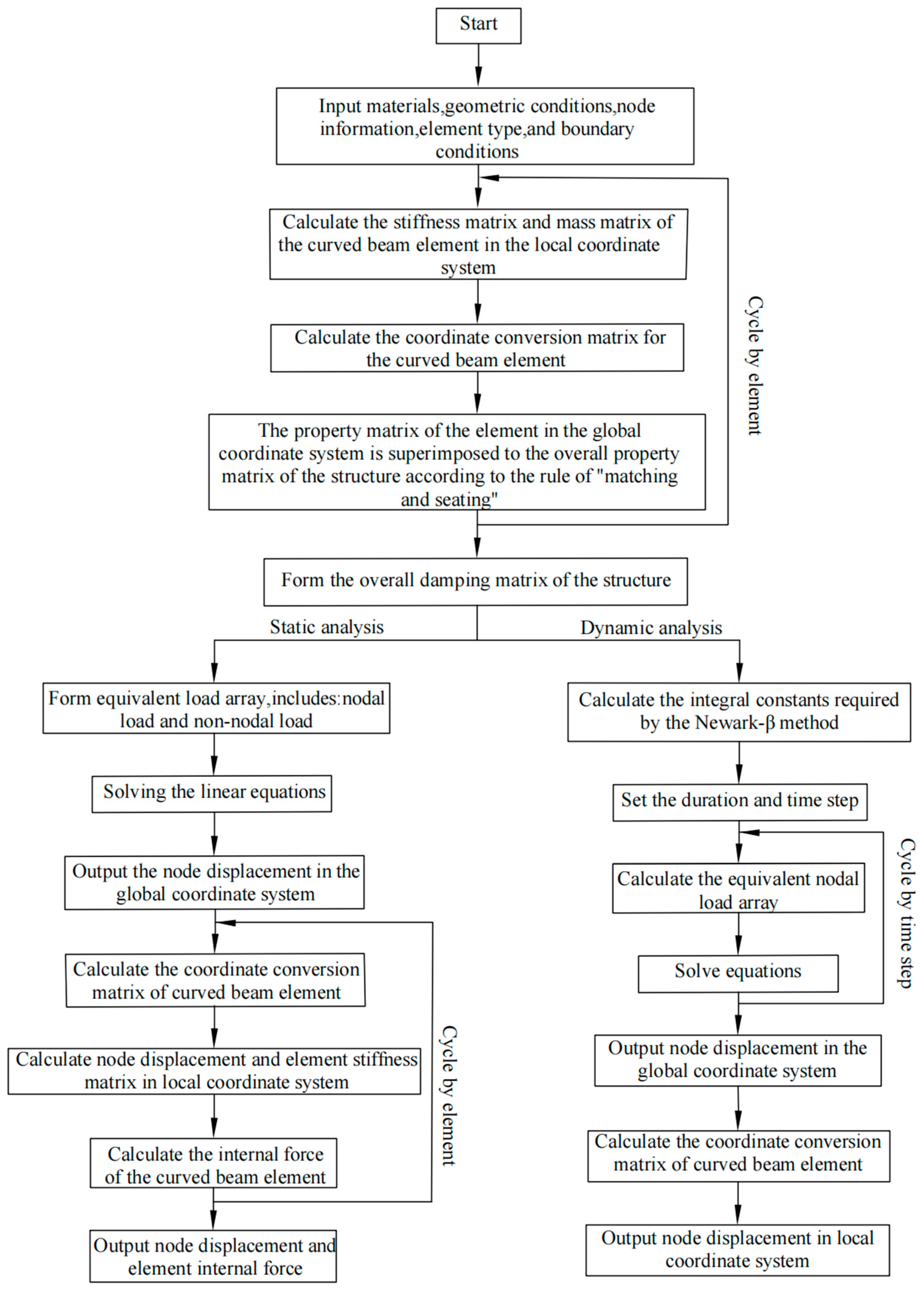
6. Development of a Finite Element Analysis Program for Quadrilateral Beam Elements in Curved Beams

When conducting numerical analysis of structures using the finite element method, the following procedure is employed. First, utilizing the coordinate transformation matrix, the local element characteristic matrix and nodal load vector are transformed from a local coordinate system into a global coordinate system. Subsequently, in accordance with the “matching” principle, these transformed matrices and vectors are assembled to form an overall structural characteristic matrix and a total nodal load vector. After accounting for prescribed boundary conditions, the displacements of unknown nodes are computed. The displacements obtained from solving the system of equations are based on the global coordinate system and need to be transformed back into the local element coordinate system before outputting the results.

Following this, the internal forces within each element are calculated using the element stiffness matrix. Finally, based on the output results, further analysis and research on the obtained data are performed. Utilizing the derived curved beam element stiffness matrix, consistent mass matrix, and coordinate transformation matrix, a finite element analysis program for curved beam elements is developed using the Fortran programming language. The static and dynamic analysis workflow is illustrated in Figure 3, in accordance with the finite element analysis methodology.

7. Validation of the Quadrilateral Beam Element Characteristic Matrix for Curved Beams: Numerical Examples

7.1. Model Development and Validation for Civil Engineering Applications

A simply supported curved box girder bridge was chosen as the research object. The bridge has a span of L = 24 m, a curvature radius of R = 100 m for the beam axis, an elastic modulus of E = 3.25 × 1010 N/m², a shear modulus of G = 1.35 × 1010 N/m², and a density of ρ = 2600 Kg/m³ for the concrete materials used. The main beam section is a single-box single-cell box girder section, as illustrated in Figure 4. It has an area of A = 4.392 m², second moments of area I_y = 2.443 m⁴ and I_z = 20.721 m⁴, and a torsional moment of inertia J = 5.042 m⁴. The bridge model’s boundary conditions were set based on the constraints of a simply supported beam.

To validate the theoretical deductions and the self-developed program, three finite element models of a simply supported curved box beam were created [24]. Model 1 used ANSYS solid elements (SOLID45) to simulate a curved beam bridge, employing regular hexahedral elements. The solid model consisted of a total of 960 elements and 2000 nodes, as depicted in Figure 5. Model 2 employed an “approximate curve with straight” approach using ANSYS beam elements (BEAM189) to discretize the simply supported curved box beam. Model 2 consisted of 24 elements and 49 nodes. Model 3 was a curved beam element model, for which input data files were generated using a self-developed program with bridge structure parameters. Two types of curved beam element model were defined in the input data files: Euler and Timoshenko models. These models were labeled as the E-curved beam element model and T-curved beam element model, respectively.

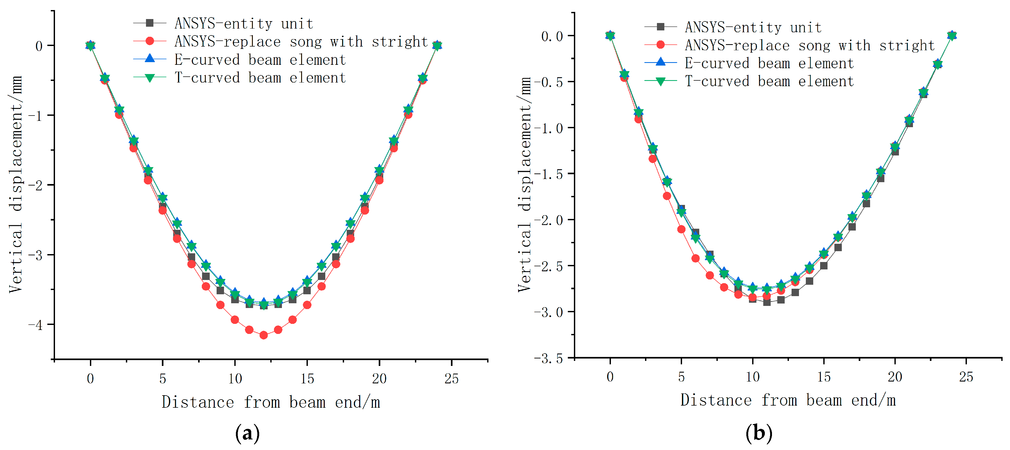
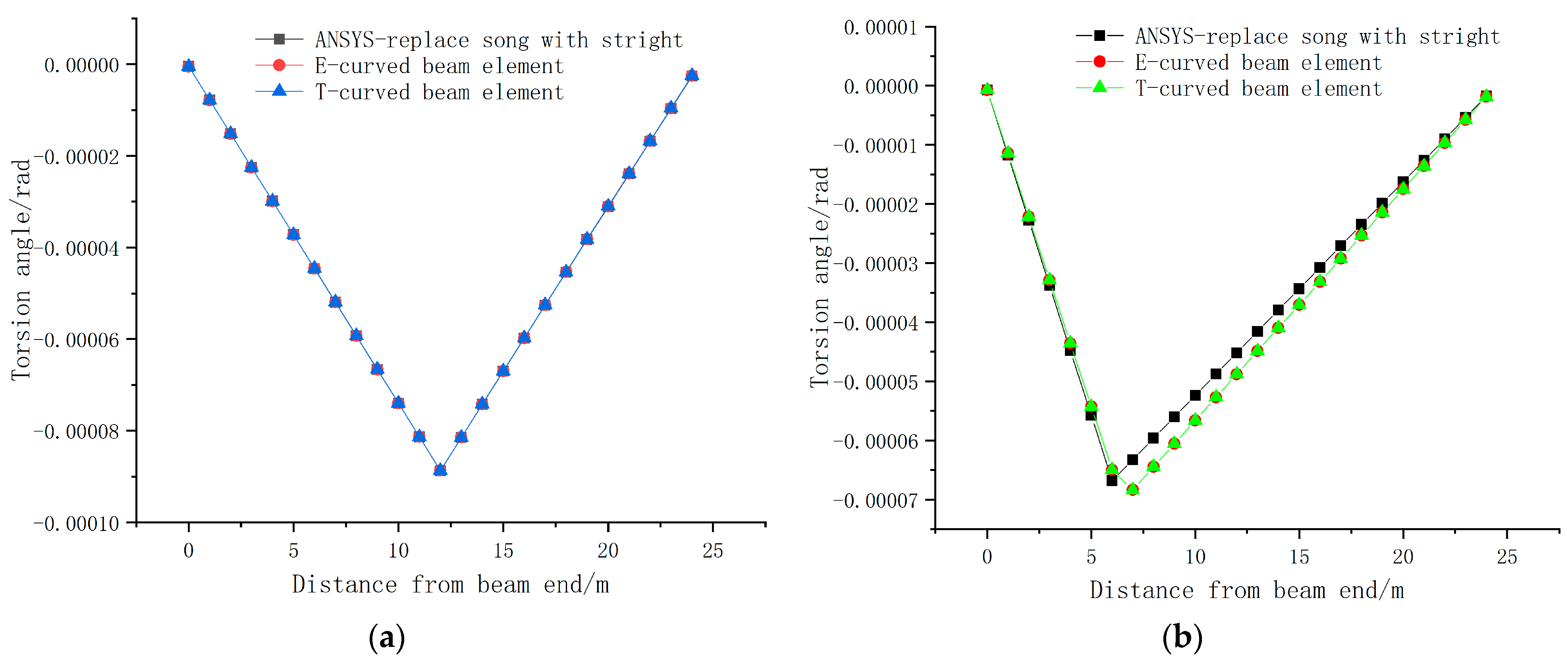
7.2. Analysis of Results for Civil Engineering Applications: Static Analysis

Under two load conditions, namely nodal loads and non-nodal loads, a lateral force (F = 1 × 10⁶ N), a vertical force (F = 1 × 10⁶ N), and a torsional moment (M = 1 × 10⁶ N·m) were applied at the node of the centerline of the top plate in the mid-span position and at a non-node position located L/4 away from the beam end. The calculated main beam displacements for the different analysis models of the curved beam bridge are presented in Figure 5, Figure 6, Figure 7 and Figure 8, and the peak displacement values are compared in

Table 1. Peak Displacement of the Different Models.

Element Type		3D Solid Model in ANSYS	Beam Element Model in ANSYS	Euler–Bernoulli Beam Element Model	Timoshenko Beam Element Model
Node Load	Lateral Displacement (unit in mm)	0.168	0.296	0.128	0.189
	Vertical Displacement /mm	3.734	4.160	3.695	3.717
	Twist Angle/(×10−5 rad)	--	8.873	8.868	8.868
Non-Node Load	Transverse Displacement/mm	0.110	0.187	0.079	0.121
	Vertical Displacement/mm	2.900	2.850	2.750	2.759
	Twist Angle/(×10−5 rad)	--	6.679	6.836	6.836

, while the computation times for the four models under static analysis are provided in

Table 2. Computational Time of the Various Models in the Static Analysis.

Element Type	Node Load (s)	Non-Node Load (s)
3D solid model in ANSYS	1	1
Beam element model in ANSYS	1	1
Euler–Bernoulli beam element model	0.9	0.9
Timoshenko beam element model	0.9	0.9

.

From Figure 6, it is apparent that the lateral displacements obtained from the Timoshenko curved beam element model and the ANSYS solid model were in good agreement, with similar peak values. The lateral displacement of the Euler curved beam model was slightly smaller. This can be attributed to the fact that the Euler curved beam element neglects the influence of transverse shear deformation, resulting in a stiffer response in the lateral direction. On the other hand, the “straight replacement for curved” ANSYS beam element model exhibited a larger lateral displacement, indicating that using the “straight replacement for curved” method decreased the lateral stiffness of the curved beam element, due to neglecting bending–torsion coupling effects.

From Figure 7 and Figure 8, and Table 1 and Table 2, it can be observed that the vertical displacements and torsional displacements of the different analysis models exhibit similar trends. Additionally, the computation times of the various models were also generally comparable.

The vertical displacements of the Euler and Timoshenko curved beam element models closely matched those of the ANSYS solid model, while the “straight replacement for curved” beam element model yielded larger vertical displacements compared to the other three models. The torsional displacements of the Euler and Timoshenko curved beam element models were consistent and slightly larger than the calculated values of the “straight replacement for curved” beam element model under non-nodal loads.

Since the solid model accurately represented the mass and stiffness distribution of the curved beam bridge, and as the results obtained from the curved beam element models were in good agreement with the solid model, this indicates that the derived stiffness matrix for the curved beam element in this study was correct and can be utilized for static analysis of curved beam bridges.

Analysis of Natural Frequencies and Modes for Civil Engineering Applications

The natural frequencies of a structure provide valuable insights into its mechanical characteristics, and they can be used to validate the correctness of the stiffness matrix and mass matrix of a curved beam element. In this study, the subspace iteration method was employed to analyze the natural frequencies of the aforementioned bridge models, and the first five natural frequencies with the same mode shape were extracted for comparison. The calculated results are presented in

Table 3. Natural Frequencies and Mode Shape Characteristics of the Different Models.

Order	3D Solid Model in ANSYS	Beam Element Model in ANSYS	Euler–Bernoulli Beam Element Model	Timoshenko Beam Element Model	Vibration Mode Characteristics
1	6.88	6.86	7.21	7.19	Symmetric vertical bending
2	23.46	24.13	24.22	23.96	Antisymmetric vertical bending
3	29.95	29.57	31.64	30.16	Lateral bending
4	36.69	36.51	36.71	36.54	Vertical displacement
5	45.79	46.12	47.53	47.52	Torsion

.

From the results presented in Table 3, it is evident that the calculated natural frequencies of the Euler and Timoshenko curved beam element models, as well as the “straight replacement for curved” ANSYS beam element model, exhibited good agreement with the ANSYS solid model. The calculated mode shapes for modes such as vertical bending, lateral bending, longitudinal translation, and torsion were also consistent among the different models. The frequencies obtained from the Euler and Timoshenko curved beam element models were slightly higher, with most deviations falling within 5%. This further confirms that the derived stiffness and mass matrices for the curved beam element in this study accurately captured the mechanical characteristics of the curved beam bridge.

7.3. Analysis of Results for Civil Engineering Applications: Dynamic Analysis

A concentrated mobile load of F = 1 × 10⁶ N was applied to a curved beam bridge at a constant speed of v = 10 m/s. To investigate the effects of moving loads on curved beam bridges, a dynamic analysis was conducted on several models. Time history curves for vertical displacement and twist angle were then calculated at the mid-span of the curved beam bridge, as represented in Figure 9 and Figure 10. Under dynamic analysis, the computation times for different models are provided in

Table 4. Computation Time of Different Models in Dynamic Analysis.

Element Type	Time (s)
3D solid model in ANSYS	1.2
Beam element model in ANSYS	1.2
Euler–Bernoulli beam element model	1.5
Timoshenko beam element model	1.5

.

From Figure 9 and Figure 10 and Table 4, it is evident that the dynamic analysis results exhibited the same patterns as observed in the static analysis. The overall trends in the vertical displacement and torsional displacement over time among the different analysis models remained roughly consistent. The computation time was slightly higher compared to the static analysis; however, the calculation times for the three models were still roughly similar. Specifically, the vertical displacement values of the Euler and Timoshenko curved beam element models closely aligned with those of the ANSYS solid model. Conversely, the “straight instead of curve” beam element model displayed a larger vertical displacement. Furthermore, the twist displacement time history curve at the mid-span demonstrated excellent agreement, indicating that the characteristic matrix derived for the curved beam element in this study possesses strong adaptability and is suitable for dynamic analysis of curved beam bridges.

In conclusion, through a comparison of static, modal, and dynamic analysis results using different analysis models (ANSYS solid element, “straight instead of curve” ANSYS beam element, and Euler and Timoshenko curved beam element), it can be concluded that the ANSYS solid element model accurately represented the mechanical characteristics of the curved beam bridge. The results obtained from the curved beam element model exhibited good agreement with the solid model, thereby validating the accuracy and applicability of the derived characteristic matrix for the curved beam element in this study. Additionally, the use of curved beam elements in the numerical analysis of curved beam bridges offers the advantage of reducing the overall degree of freedom of the structure, resulting in faster and more convenient calculations.

8. Conclusions

This study primarily concerned curved beam bridges and presented the derivation of an element stiffness matrix, element consistent mass matrix, and coordinate transformation matrix based on the displacement distribution pattern of trigonometric functions. A finite element analysis program was developed using the programming language Fortran. Static and dynamic analyses, as well as free vibration analyses, were carried out on a curved beam element. The outcomes were compared with the solid model in ANSYS APDL 19.2 software and the “straight-substituted-curved” beam element model, which validated the findings. The study concluded that the developed analysis program is capable of performing accurate simulations of curved beam structures.

• The computed results from both the Euler and Timoshenko curved beam element models exhibited an excellent correlation with the solid model in ANSYS software, thus confirming the accuracy of the characteristic matrix derived for the curved beam element in this study;
• The vertical displacement of the “straight-substituted-curved” beam element model was consistently higher, implying that the “straight-substituted-curved” approach resulted in a decrease in the vertical stiffness of the curved beam. This reduction can be attributed to the neglect of the bending–torsion coupling effect in the simulation of the curved beam bridge using this approach;
• The utilization of curved beam elements for numerical analysis of curved beam bridges can noticeably diminish the total degree of freedom, enhancing the computational speed and convenience, while facilitating the advancement of computational programs, thus rendering this an exceptionally beneficial approach for modeling curved beam bridges and extending research on topics such as vehicle–bridge coupling vibration for curved beam bridges, which require a high degree of accuracy and computational efficiency to achieve optimal results;
• This study demonstrates that the displacement distribution model based on trigonometric functions employed in the finite element analysis of curved beam elements exhibited a relatively limited scope. Subsequent investigations should encompass the utilization of diverse models for the purpose of validation and analysis.

References

1. Zhou, L.; Liu, Z.; Yan, X.; Li, Q. Design Theory and Analytical Methods for Curved Beam Bridge Structures; People’s Communications Press: Beijing, China, 2018. [Google Scholar]
2. Edita, D.; Bořek, P. An isogeometric Timoshenko curved beam element with an enhanced representation of concentrated loads. Comput. Struct. 2022, 270, 106815. [Google Scholar]
3. Rezaiee-Pajand, M.; Rajabzadeh-Safaei, N.; Masoodi, R.A. An efficient mixed interpolated curved beam element for geometrically nonlinear analysis. Appl. Math. Model. 2019, 76, 252–273. [Google Scholar] [CrossRef]
4. Dragan, R. A Simple and Efficient Three-Node Curved Beam Element for the Out-of-Plane Shear, Bending and Torsion, Based on the Linked Interpolation Concept. Trans. Famena 2021, 45, 13–29. [Google Scholar]
5. Zhang, Z. Theoretical Research and Application of Qu-Liang Element in Bridges. Master’s Thesis, Changsha University of Science and Technology, Changsha, China, 2014. [Google Scholar]
6. Luo, H. Analysis and Research on the Mechanical Properties of Curved Beam Bridges. Master’s Thesis, Chang’an University, Xi’an, China, 2014. [Google Scholar]
7. Macedo, R.C.; Marcos, A.; Dalledone, R.M. Free in-plane vibration analysis of curved beams by the generalized/extended finite element method. Eur. J. Mech. A Solids 2021, 88, 104244. [Google Scholar]
8. Jočković, M.; Radenković, G.; Nefovska-Danilović, M.; Baitsch, M. Free vibration analysis of spatial Bernoulli–Euler and Rayleigh curved beams using isogeometric approach. Appl. Math. Model. 2019, 71, 152–172. [Google Scholar] [CrossRef]
9. Gao, Y.; He, G.; Zhou, W. Finite element analysis of plane curved beam. West China Explor. Eng. 2005, 6, 188–190. [Google Scholar]
10. Zhou, W.; Zeng, Q. Geometric nonlinear finite element analysis of spatial curved beams. J. Chang. Railw. Univ. 1998, 3, 1–5. [Google Scholar] [CrossRef]
11. Wu, Y.; Lai, Y.; Zhang, X.; Zhu, Y. Analysis of static and dynamic characteristics of curved box girder by finite segment element. J. China Railw. Soc. 2001, 5, 81–84. [Google Scholar]
12. Guo, W.; Ding, M.; Deng, T.; Jiang, X.; Wang, B.; Huang, Z. Direct Stiffness Method for Static Analysis of Circular Arch Structures. J. Guangxi Univ. 2017, 42, 1351–1360. [Google Scholar]
13. Nadi, A.; Raghebi, M. Finite Element Model of Circularly Curved Timoshenko Beam for In-plane Vibration Analysis. FME Trans. 2021, 49, 615–626. [Google Scholar] [CrossRef]
14. Chen, J. Stiffness Matrix and Consistent Mass Matrix of Element for Curved Beam Displacement Field Function. Transp. Stand. 2008, 2008, 51–54. [Google Scholar]
15. Li, X.; Li, P.; Sun, L. Decoupling Solution Method and Verification of Free Vibration Differential Equations for Curved Beams. Nucl. Power Eng. 2016, 37, 7–10. [Google Scholar]
16. Rezaiee-Pajand, M.; Rajabzadeh-Safaei, N. An explicit stiffness matrix for parabolic beam element. Lat. Am. J. Solids Struct. 2016, 13, 1782–1801. [Google Scholar] [CrossRef]
17. Lebeck, A.O.; Knowlton, J.S. A finite element for the three-dimensional deformation of a circular ring. Int. J. Numer. Methods Eng. 1985, 21, 421–435. [Google Scholar] [CrossRef]
18. Wu, J.S.; Chiang, L.K. A new approach for free vibration analysis of arches with effects of shear deformation and rotary inertia considered. J. Sound Vib. 2004, 277, 49–71. [Google Scholar] [CrossRef]
19. Wu, J.S.; Chiang, L.K. A new approach for displacement functions of a curved Timoshenko beam element in motions normal to its initial plane. Int. J. Numer. Methods Eng. 2005, 64, 1375–1399. [Google Scholar] [CrossRef]
20. Kim, J.G.; Lee, J.K. Free-vibration analysis of arches based on the hybrid-mixed formulation with consistent quadratic stress functions. Comput. Struct. 2007, 86, 1672–1681. [Google Scholar] [CrossRef]
21. Desantiago, E.; Mohammadi, J.; Albaijat, H. Analysis of horizontally curved bridges using simple finite-element models. Pract. Period. Struct. Des. Constr. 2005, 10, 18–21. [Google Scholar] [CrossRef]
22. Zhang, J.; Yin, H.; Li, J.; Chen, H. Derivation of Stiffness Matrix for Euler-Bernoulli Beam Element. J. Water Resour. Archit. Eng. 2019, 17, 89–93+131. [Google Scholar]
23. Jiang, T. Key Technologies for Design of Curved Beam Bridges and Experimental Study of Model. Master’s Thesis, Dalian University of Technology, Dalian, China, 2021. [Google Scholar]
24. Chen, P.; Du, H.; Sun, S.; Fu, X. Unified Formation Method of General Beam Element in Finite Element Software. Mech. Eng. Pract. 2021, 43, 446–452. [Google Scholar]
Figure 1. Local and global coordinate systems, node displacements, and internal forces of curved beam elements; (a) in-plane vibration; (b) out-of-plane vibration.
Buildings 13 02239 g001
Figure 2. Transformation relationship between global and local coordinate systems for a curved beam element.
Buildings 13 02239 g002
Figure 3. Finite element analysis workflow for a curved beam element.
Buildings 13 02239 g003
Figure 4. Section dimensions of the box beam (unit: cm).
Buildings 13 02239 g004
Figure 5. Three-dimensional finite element solid model of SOLID45.
Buildings 13 02239 g005
Figure 6. Lateral displacement of the different models: (a) lateral displacement under nodal load; (b) lateral displacement under non-nodal loading.
Buildings 13 02239 g006
Figure 7. Vertical displacement of different models: (a) vertical displacement under nodal loading; (b) vertical displacement under non-nodal loading.
Buildings 13 02239 g007
Figure 8. Comparison of the torsional displacement of the different models: (a) torsional displacement under nodal loading; (b) torsional displacement under non-nodal loading.
Buildings 13 02239 g008
Figure 9. Vertical displacement time history of mid-span.
Buildings 13 02239 g009
Figure 10. Twist displacement time history of mid-span.
Buildings 13 02239 g010