Experiment and Prediction of Pressure Drop in a Fiber–Powder Composite Material with Porous Structure for Energy Wheels and Air Cleaners

Abstract

Energy wheels and air cleaners play crucial roles in building air conditioning systems. The former is essential for conserving energy in air conditioning systems, while the latter is necessary for ensuring the quality of indoor air. Pressure drop is a crucial parameter for both energy wheels and air cleaners, and it is essential to conduct theoretical and experimental investigations to aid in their design. In this study, we focused on the study of pressure drop in a fiber–powder composite material which can be used for both total heat exchange and air purification. Experimental tests were initially conducted to examine the impact of different parameters on the pressure drop in the material. Subsequently, based on the special fiber–powder structure of the material, two pressure drop prediction methods with different prediction strategies were proposed. The two prediction strategies were compared by analyzing the prediction accuracy of the two methods. As tested by experimental data, for both methods, the absolute prediction error was less than ±6 Pa when the pressure drop was below 50 Pa, and the relative prediction error was less than ±8% for most data sets when the pressure drop was greater than 50 Pa. Moreover, the root mean square error ($RMSE$) and mean absolute percentage error ($MAPE$) values of prediction for both methods were less than 4 Pa and 7% respectively. The test results show that although the prediction strategies are different, both prediction methods can obtain acceptable prediction results, and both methods are practical. This study is intended to serve as a valuable reference for the design of energy wheels and air cleaners.

1. Introduction

Energy wheels play a significant role in building energy conservation because they can reduce the fresh air load of air conditioning systems by recovering energy from indoor air. The results of previous experiments [1,2] have demonstrated the effectiveness of energy recovery wheels in reducing the fresh air load in both cold and hot climates. Figure 1 illustrates the working principle of energy wheels. Air cleaners are also widely used in building applications, where they play a key role in maintaining and improving the indoor air quality.

For energy wheels and air cleaners, the pressure drop is a critical parameter that significantly impacts the design of these devices. Therefore, it is meaningful to establish pressure drop prediction models to study the pressure drop of these devices. In [3,4,5], pressure drop models for energy wheels or rotary heat exchangers were developed, and they were utilized to investigate the thermal performance of the wheel. Moreover, in [6,7,8], pressure drop models for adsorption filters or air filters were developed for better design of the device. Dallaire et al. [4] examined the influence of a dimensionless pressure drop on the optimal values of two design variables of a rotary heat exchanger with a porous medium. Their findings indicated that the optimal length of the device is strongly affected by the dimensionless pressure drop. Harshe et al. [5] constructed pressure drop and heat and mass transfer models of desiccant wheels which can be utilized for energy recovery. In their study, heat and mass transfer coefficients were obtained by assuming that the Stanton number is proportional to the fractional coefficient. Zhang et al. [6] studied the pressure drop of honeycomb adsorption filters filled with granular adsorbents and built a prediction model of the filter. It was found that the pressure drop was mainly affected by the void ratio and the granular size and shape of the material.

The material investigated in this study features a porous structure with a fibrous material serving as the substrate material, which is sprayed with adsorption material powder. Previous studies have shown that the material with this structure has good total heat exchange performance [9], which can be considered to be a potential high-performance energy wheel core material. In addition, the composite material can be used for air purification, as the sprayed adsorption material can absorb contaminants. As a result, the material is versatile and can be applied in a wide range of building applications, and it is meaningful to study its pressure resistance characteristics.

Studies have been conducted on the pressure drop of fibrous materials [10,11,12,13,14,15,16,17] and granular matrices [18,19,20,21], which contain experimental investigations and modeling of the materials’ pressure drop. These studies can serve as a reference for the establishment of pressure drop models for porous materials. Liu et al. [10] developed a friction factor correlation of foam matrixes using experimental pressure drop data and found that the friction factor of granular matrixes is far more than that of foam matrixes. Watanabe et al. [11] studied pressure drop and heat transfer in a sintered fibrous porous media. In their study, the friction factor of the heat transfer tube was calculated, and a pressure drop model containing a quadratic function of velocity was built.

In the above research, the influence of various variables on the pressure resistance characteristics of porous materials was explored. For the prediction of pressure drop, it is important to know the relationship between various parameters and the materials’ pressure drop. Wang et al. [17] simulated the pressure drop in a fibrous air filtration material and compared it with experimental results. An exponential relationship between the pressure drop and the fiber diameter and porosity of the material was found. Allen et al. [18] investigated the effect of different variables on packed bed pressure drop experimentally. Results showed that when building the pressure drop prediction model, the particle shape, surface roughness, and packing method of the material should be taken into consideration, because these factors have significant effects on pressure drop. Koekemoer and Luckos [19] studied the influence of particle size distribution and material type on the pressure drop of packed beds. In their study, the Ergun equation was modified to predict the pressure drop of packed beds filled with particles of multiple materials, and good prediction results were obtained.

However, most of the existing studies on pressure drop in porous materials have focused on porous material with a single medium, which means that the material does not possess a composite structure. Theoretical and experimental investigations on the pressure drop characteristics of fiber–powder composite materials are relatively rare. Due to both fiber and powder having impacts on the pressure drop of the material, the influence of both of them on the pressure drop needs to be considered when building a pressure drop prediction model.

The present study is aimed at studying the pressure drop in a fiber–powder composite material. Moreover, the study tries to find a high-accuracy pressure drop prediction method suitable for the studied material. Considering the specificity of the material structure, this paper tries to split the prediction of the pressure drop into several steps to accomplish it. As a result, the proposed prediction methods of the material are different from traditional prediction methods for porous material. The study began with an experimental investigation of the pressure drop of the composite material to study the impact of various parameters on the material’s pressure drop. After that, a multi-step method for predicting the pressure drop of the material was proposed. The method divides the pressure drop of the material into two parts and predict them separately to increase prediction accuracy. After that, another prediction method with different prediction strategies was proposed; the method predicts the pressure drop of the material using one model but trained in two steps. The accuracy of the two methods was compared and their advantages were discussed. This research provides a reference for pressure drop prediction and the optimal design of energy wheels and air cleaners.

2. Methodology

In this section, the pressure drop test system and test method are introduced first. Subsequently, the pressure drop prediction models for the composite material are established, and finally, the prediction steps and methods using the built model are summarized.

2.1. Pressure Drop Experimental Setup

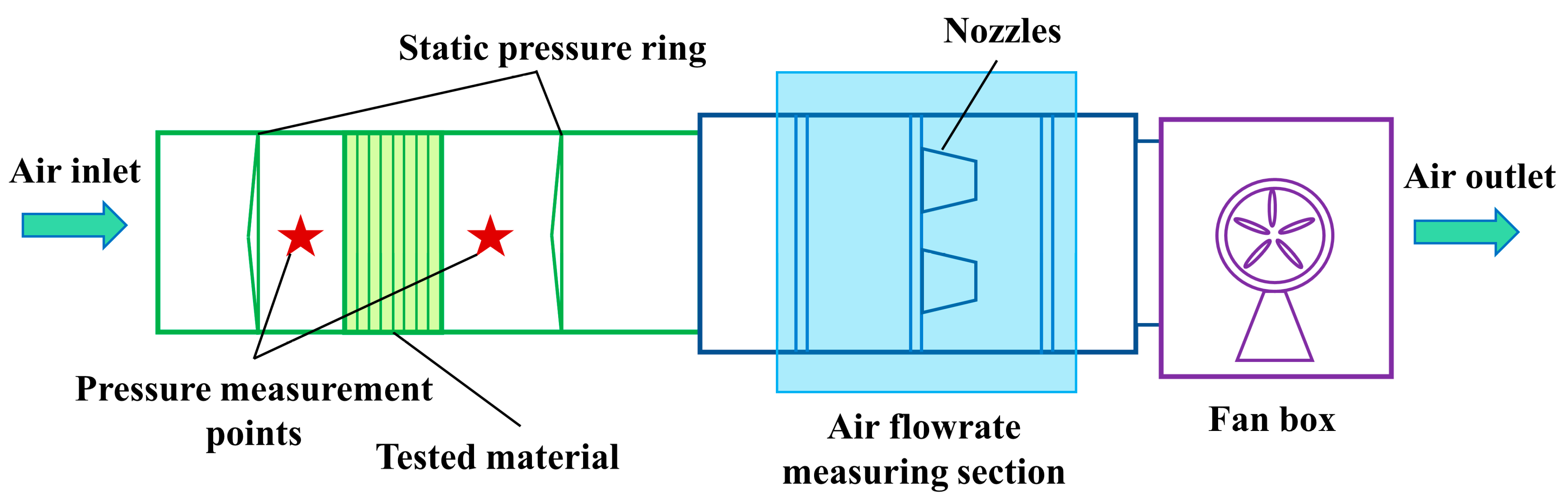
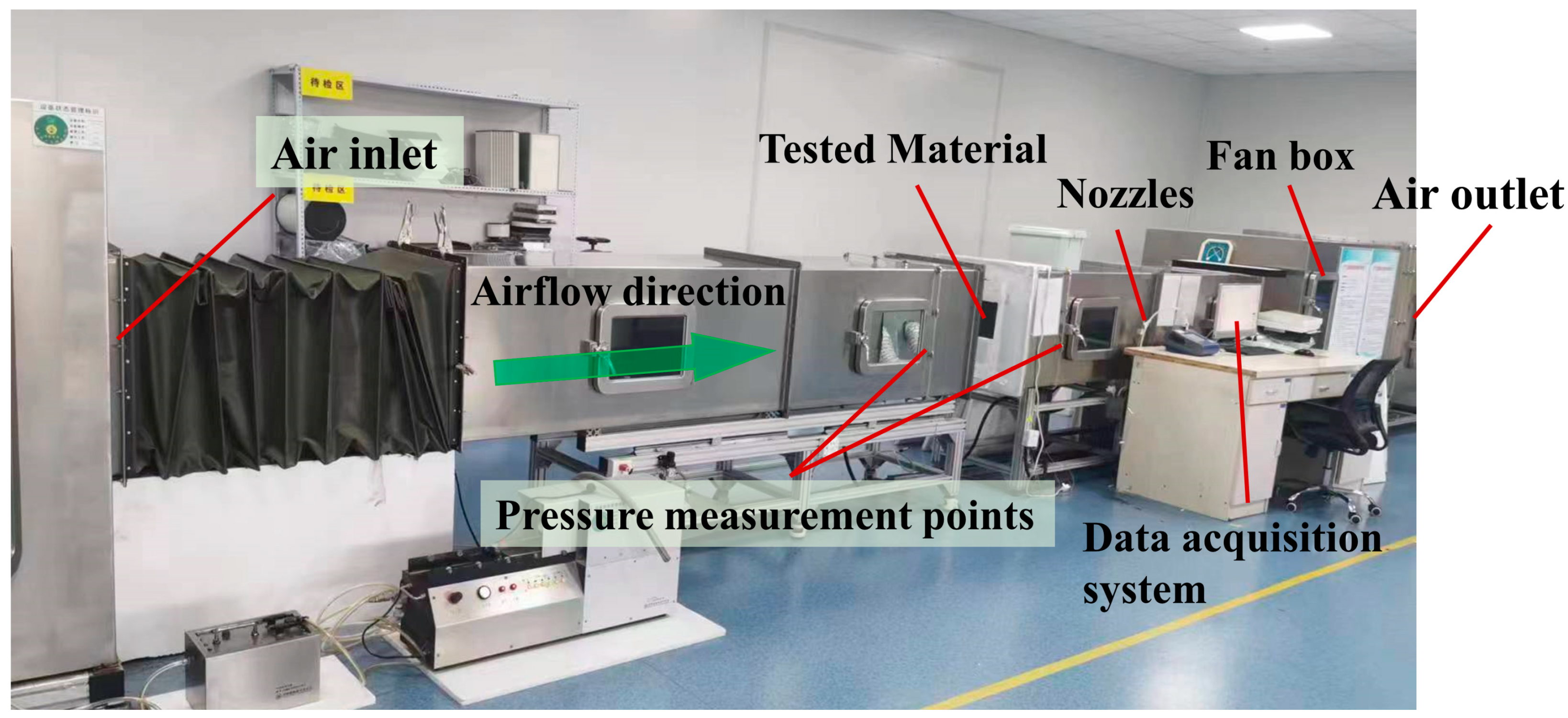
An experimental apparatus was utilized to test the air volume flowrate and pressure drop. Figure 2 and Figure 3 show the schematic diagram and physical diagram of the experimental system, respectively. The system consists of an air flowrate measuring section and a pressure drop testing section, and the measured data can be analyzed using a data acquisition system. The details of the testing method of air flowrates and pressure drop are specified in GB/T 14295-2019 [22]. The pressure drop of the material was measured using a differential pressure gauge with a range of 0–1000 Pa. During the experiment, measurement points were established on the up- and down-wind side of the tested material to obtain the pressure drop, which can be calculated using the following equation:

$$\Delta p_t=p_{t,up}-p_{t,down}$$

(1)

During the experiment, the air volume flowrate was measured using nozzles. The total air flowrate through the tested material was obtained by summing the flowrates of the individual nozzles. The air velocity could be calculated using the measured air volume flowrate and cross-sectional area. The adjustable range of air velocity in the experiment was 0.2–1.5 m/s. The air volume flowrate of one nozzle and the total air volume flowrate can be calculated using the following equations, which are in accordance with the standard [23]:

$$Q_i=Y{C}_i{F}_i\sqrt{2\Delta p_{N}u}$$

(2)

$$Q_N={{\displaystyle \sum }}_{i=1}^n{Q}_i$$

(3)

Here, $Y$ is the expansion coefficient, where $Y=0.452+0.548\left(1-\frac{\Delta p_N\times {10}^{-3}}{p_N}\right)$; $Q_i$ is the air volume flowrate through the ith nozzle; $Q_N$ is the total air volume flowrate; $F_i$ and $D_i$ are the cross-sectional area and diameter of the ith nozzle, respectively, where $F_i=\frac{\pi D_i{}^2}{4}$; $C_i$ is the flow coefficient of the ith nozzle; and $\Delta p_N$ and $p_N$ are the static pressure difference before and after the nozzle and the air pressure in front of the nozzle, respectively.

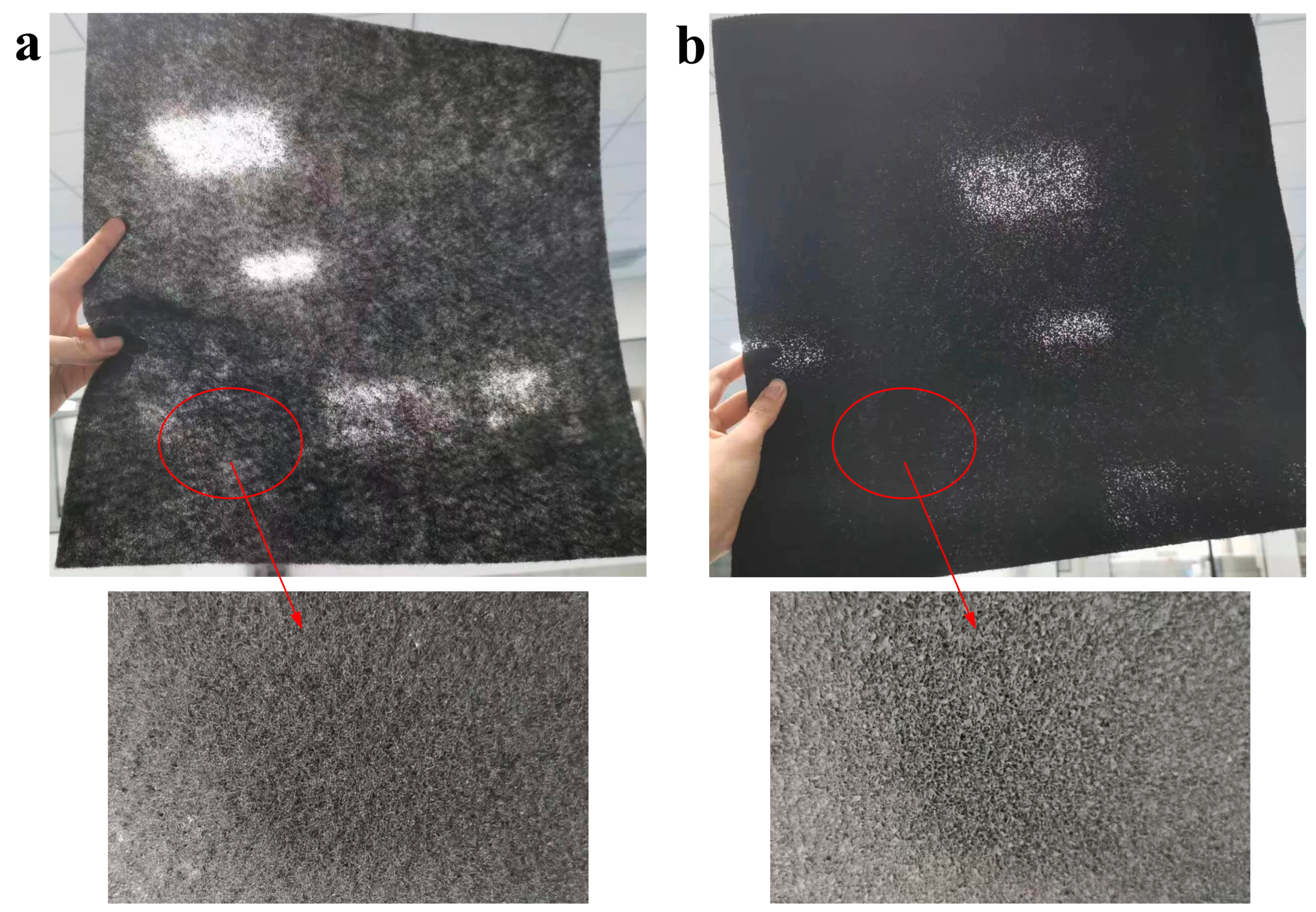
The tested material’s substrate material is composed of polyester wadding, which has a fibrous structure. The powder material is uniformly sprayed onto the surface of the polyester wadding using a spraying process. After spraying and drying, the powder material adheres to the fiber filaments inside and on the surface of the substrate material. Activated carbon powder is used as the powder material. Considering its porous structure and adsorption characteristics, it can be used as a desiccant material for total heat exchange and an adsorption material for air purification. Figure 4 displays the physical image of the substrate material before and after the activated carbon is sprayed. More details of the tested material including the morphology and adsorption properties can be found in reference [9].

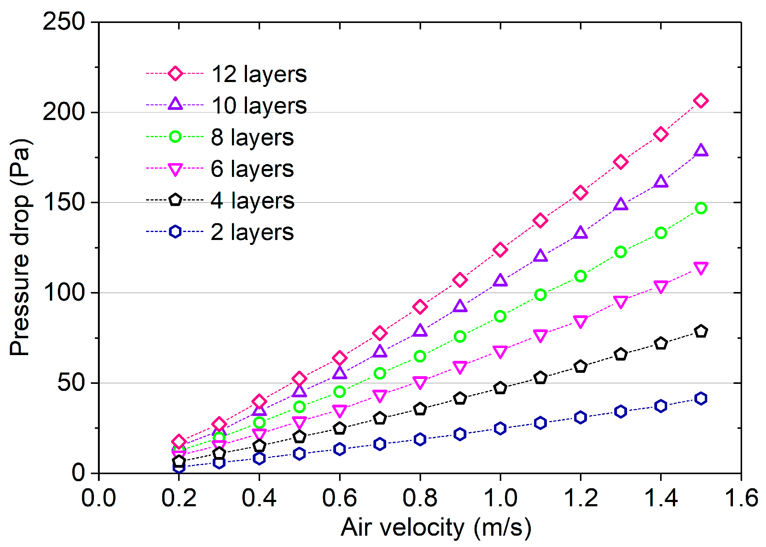
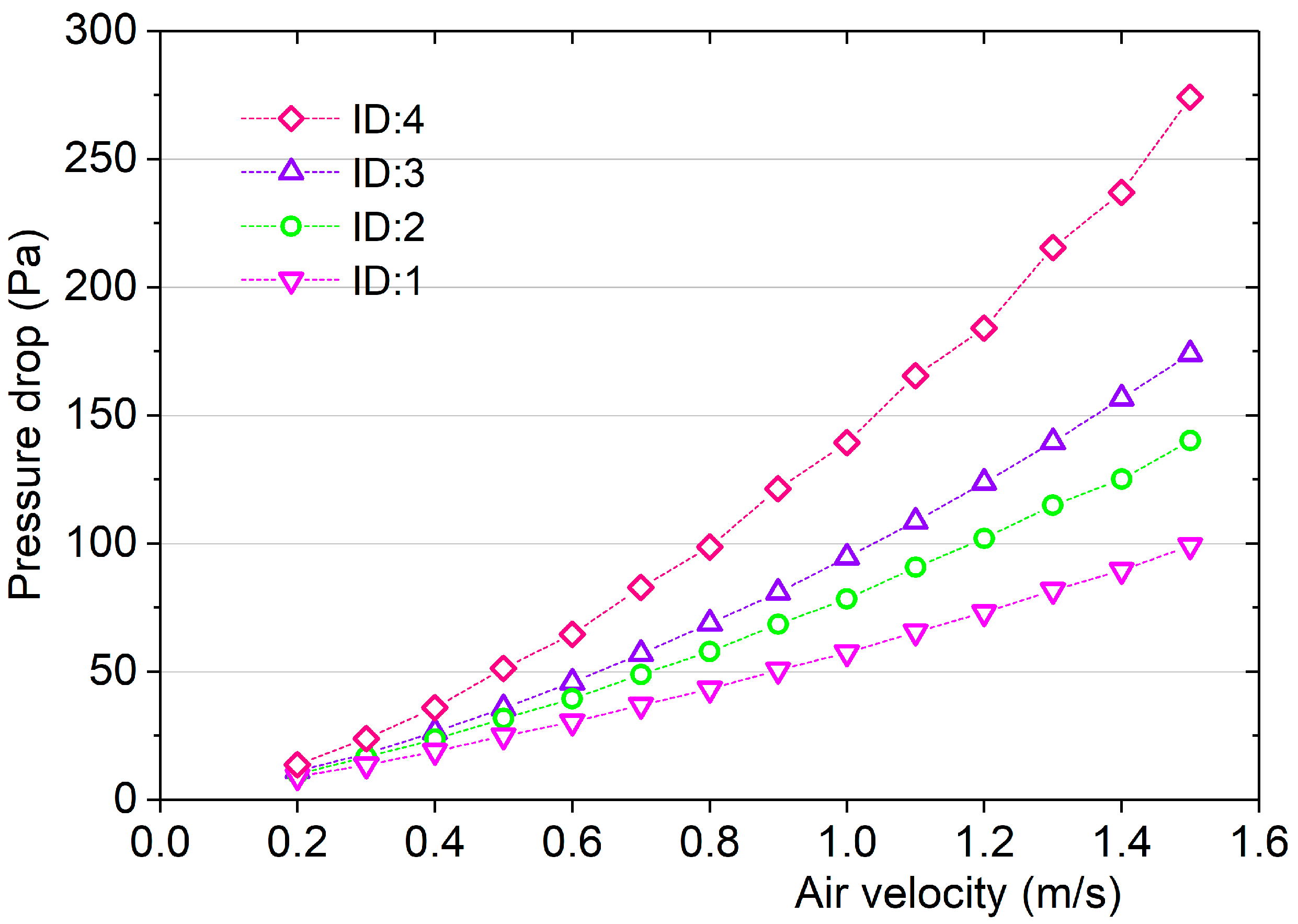
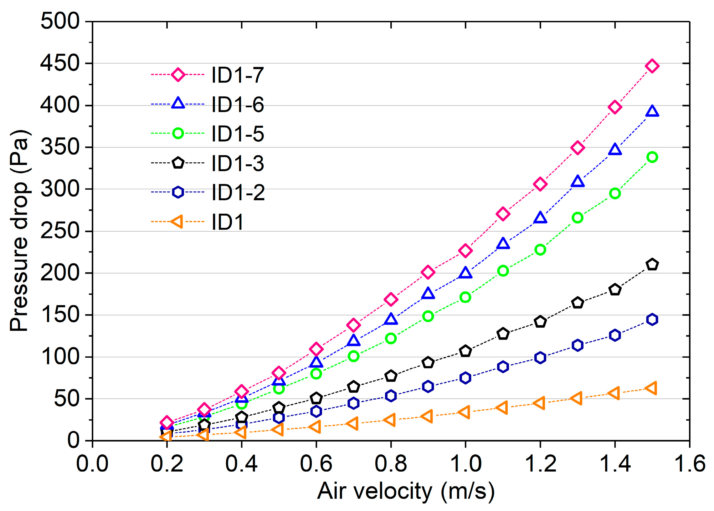
Four test materials with different amounts of carbon per unit area were prepared. All four test materials were based on the same substrate material. The thickness of the material was adjusted by changing the number of layers during the test, and the pressure drop of the multilayer materials was measured after stacking the multilayer materials together. In the experiment, the airflow passed vertically through the surface of each layer of material. The thickness and mass of a single-layer substrate material were about 3 mm and 0.027 kg, respectively.

2.2. Pressure Drop Prediction Model for the Composite Material

The main objective of this section is to establish a pressure drop prediction method capable of predicting material pressure drop under different adsorption material loading and operating conditions while using a fixed substrate. If the parameters of the substrate material are considered, more parameters will be introduced to the pressure drop prediction model. This will significantly increase the amount of experimental data needed to train the model, and the cost of experiment will be greatly increased. Moreover, the increase of parameter amounts will make the accurate prediction much more difficult. As a result, a fixed substrate is used for prediction. As the adsorption material loading increases, the pressure drop of the material increases based on the pressure drop of the substrate. This rise in pressure drop is attributed to the adhesion of adsorption materials. Given the wholly distinct shape and structure of the substrate material and adsorption material, the impact of various parameters on the substrate material pressure drop and the pressure drop increase may be different. As a result, the substrate material pressure drop and the pressure drop increase caused by adsorption materials are predicted separately, and the sum of them is calculated to obtain the total pressure drop of the material.

Figure 4 illustrates that the tested material possesses a fibrous and porous structure. Given the similarity in structure, the empirical equation of foam matrices’ friction characteristics was utilized as a reference to establish the pressure drop model. The pressure drop and the friction factor can be calculated as follows [10]:

$$\Delta p=f_f\rho L{u}^2 \frac{1-\epsilon }{D_p{\epsilon }^3}$$

(4)

$$f_f=22\frac{1-\epsilon }{Re}+0.22$$

(5)

Here, $Re$ is the Reynolds number, and the relationship between the Reynolds number and other parameters can be expressed as follows:

$$Re=\left(1-\epsilon \right)\frac{D_p\rho u}{\mu }$$

(6)

Substituting Equations (5) and (6) into (4) yields

$$\Delta p=\left(22\frac{\mu }{D_p\rho u}+0.22\right)\rho L{u}^2 \frac{1-\epsilon }{D_p{\epsilon }^3}$$

(7)

It can be seen from Equation (7) that when $\rho$ and $\mu$ are kept constant, $\Delta p$ is mainly related to $L$, $u$, $\epsilon$, and $D_p$. The void ratio of single layer material can be calculated by the following equation:

$$\epsilon =1-\frac{m_s}{{\rho }_s{V}_t}-\frac{m_d}{{\rho }_d{V}_t}$$

(8)

Here, $m_s$ and $m_d$ are the content of substrate material and adsorption material per unit area, and $V_t$ is the total volume of the material per unit area. Equation (8) shows that with a certain parameter of the substrate material and $V_t$, $\epsilon$ is only influenced by $m_d$ when ${\rho }_d$ is considered as constant.

When the parameters of the substrate material are certain, $D_p$ is mainly affected by $m_d$. By increasing the amount of adsorption material, the porosity of the material being tested is reduced, and the size of the pores within the material is also impacted. Therefore, $u$, $L$, and $m_d$ can be considered as the most significant parameters affecting $\Delta p$. Since all three of these variables are easy to obtain, it is convenient to use them to train the model.

In the modeling of the pressure drop increase caused by adsorption materials, the structure of Equation (7) is referenced, and the following considerations are included:

1.

In the $\frac{1-\epsilon }{D_p{\epsilon }^3}$ term in Equation (7), $D_p$ and $\epsilon$ are mainly affected by $m_d$, and the term is positively correlated with $m_d$. To reduce computing expenses, the term is simplified to the form of an exponential function containing $m_d$.

2.

The $D_p$ in the $22\frac{\mu }{D_p\rho u}$ term is simplified to the form of an exponential function containing $m_d$.

3.

Referring to Equation (7), power functions are used to describe the relationship between L and $\Delta p_d$ as well as the relationship between u and $\Delta p_d$.

In conclusion, the pressure drop increase prediction model is formulated as

$$\Delta p_i=k_1\left(\frac{k_2\exp \left(k_3{m}_d\right)}{u}+k_4\right)L^{k_5}{u}^{k_6}\left(\exp \left(k_7{m}_d\right)-1\right)$$

(9)

Here, $k_i$s are undetermined coefficients which can be obtained through regression; $\mu$ and $\rho$ are considered as constants and merged into $k_i$s.

The prediction methods proposed in this work are based on the substrate material with constant porosity and material parameters. Therefore, the pressure drop of the substrate material is mainly influenced by the air velocity and material thickness. The substrate material’s pressure drop prediction model was developed based on the following equation [24]:

$$\frac{\Delta p}{L}=k_{1}u+k_2{u}^2$$

(10)

The pressure drop prediction model of the substrate material is formulated as

$$\Delta p_s=(j_{1}u+j_2{u}^2)L^{j_3}{u}^{j_4}$$

(11)

Here, $j_i$s are undetermined coefficients which can be obtained through regression.

The total pressure drop of the material can be obtained by summing the pressure drop of the substrate material and the pressure drop increase caused by adsorption materials:

$$\Delta p_t=\Delta p_s+\Delta p_i$$

(12)

To simplify the modeling process and reduce the experimental data required for modeling, the pressure drop model of the substrate material can be trained first to obtain coefficients $j_i$s, and the coefficient $k_5$ in Equation (9) can be replaced by $j_3$. In this way, when training the prediction model for $\Delta p_i$, the experimental data needed in the modeling can be drastically reduced due to the reduction of one model parameter. Using this approach, the cost of modeling can be reduced significantly.

2.3. Pressure Drop Prediction Procedure

The total pressure drop of the tested material can be predicted following the steps below:

A.

Obtain the tested data for prediction ($u,L,m_d,\Delta p_s, \Delta p_t$) and calculate $\Delta p_i$.

B.

Train the substrate material pressure drop prediction model and obtain the coefficient $j_i$s.

C.

Calculate $\Delta p_s$ with the trained model.

D.

Train the adsorption material pressure drop prediction model and obtain the coefficients $k_i$s.

E.

Calculate $\Delta p_i$ with the trained model and calculate the predicted $\Delta p_t$.

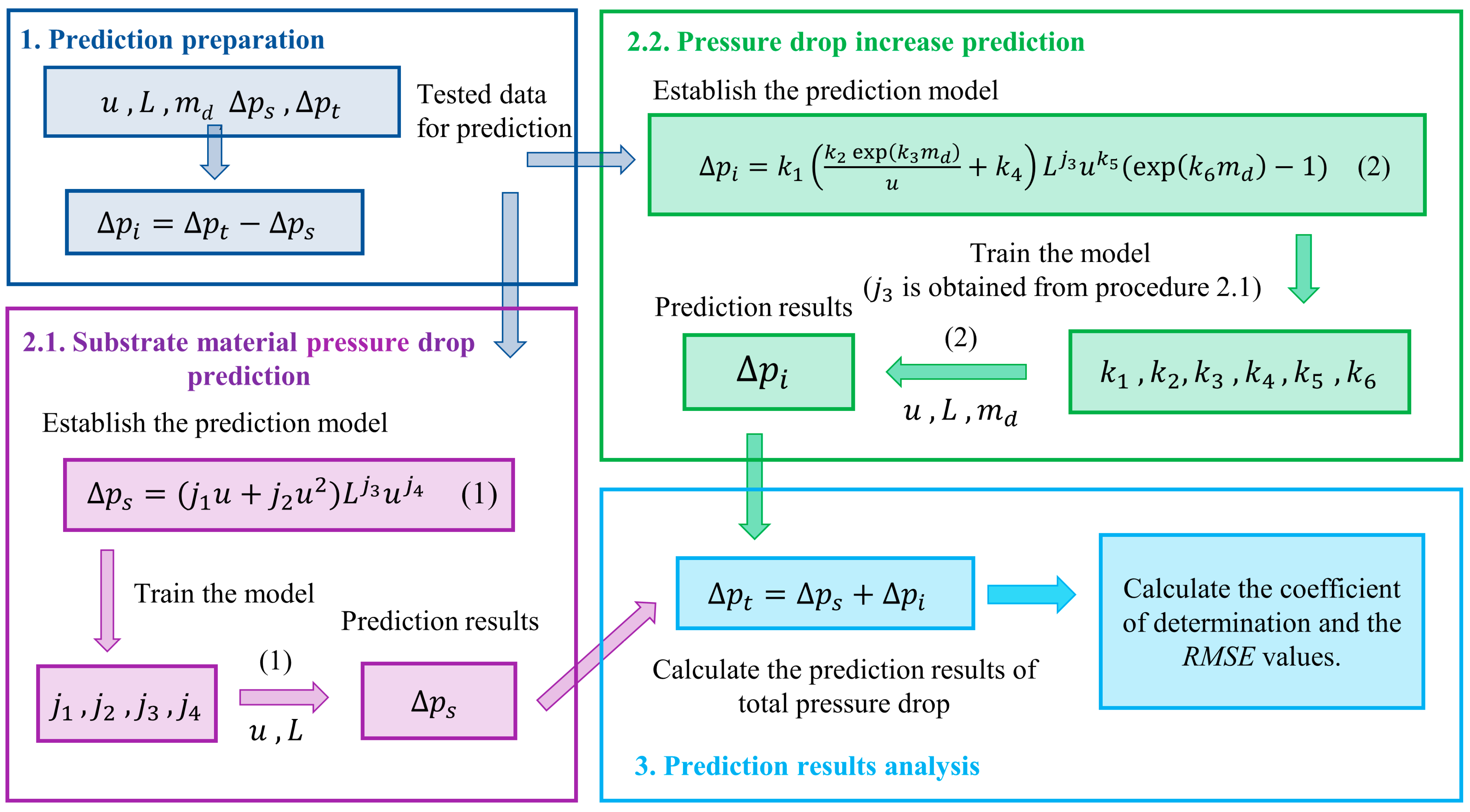
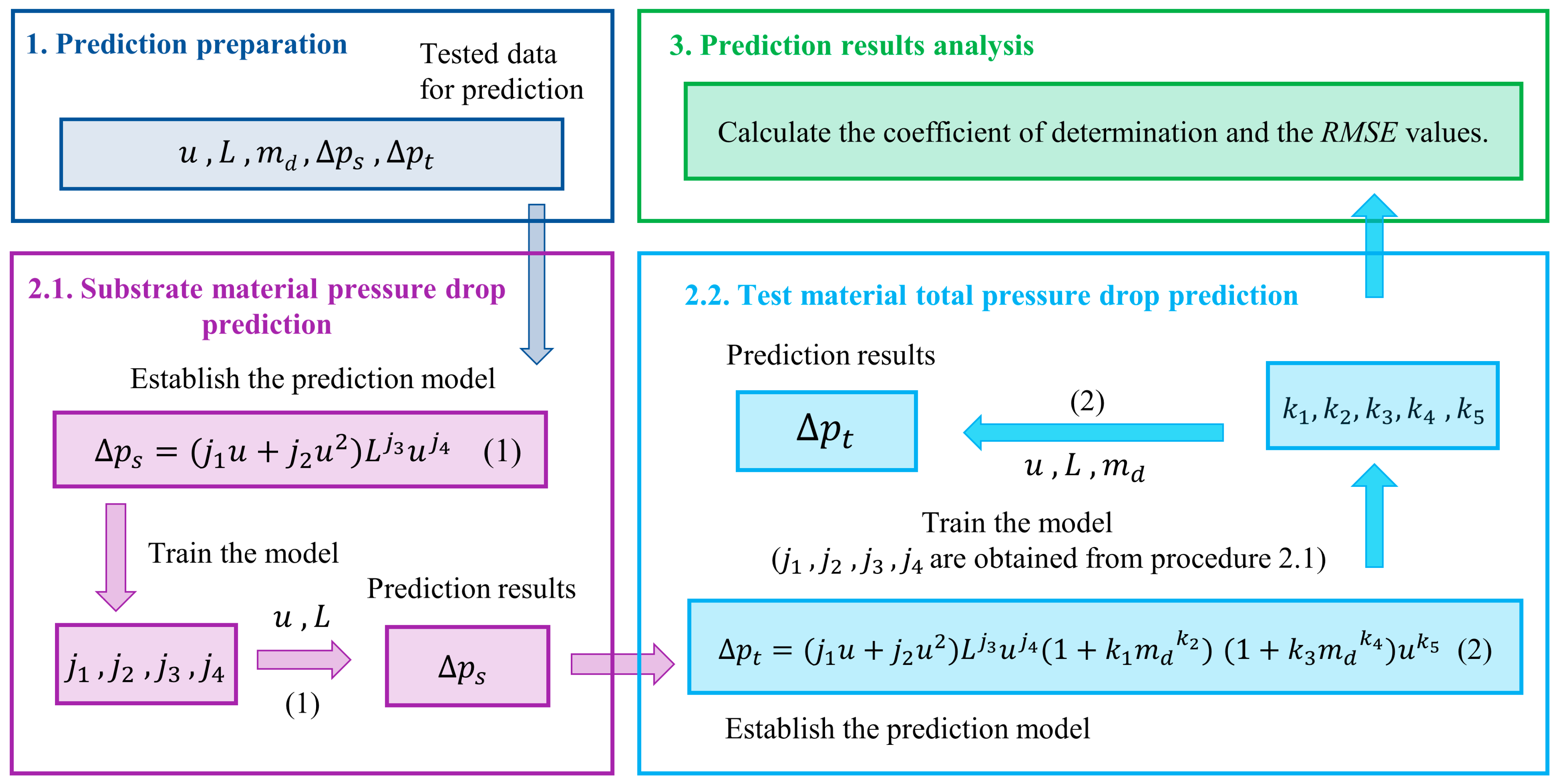
The above prediction process is depicted specifically in Figure 5. The input parameters required for training the model are specified in

Table 1. Introduction of the model input parameter.

Parameter	Acquisition Method	Use
Length of material (L)	Measured	Train the $\Delta p_s$ and $\Delta p_i$ prediction model
Air velocity (u)	Measured	Train the $\Delta p_s$ and $\Delta p_i$ prediction model
Desiccant material content ($m_d$)	Measured	Train the $\Delta p_i$ prediction model
Substrate material pressure drop ($\Delta p_s$)	Measured	Train the $\Delta p_s$ and $\Delta p_i$ prediction model
Material total pressure drop ($\Delta p_t$)	Measured	Train the $\Delta p_i$ prediction model
Material pressure drop increase ($\Delta p_i$)	Calculated	Train the $\Delta p_i$ prediction model

.

Experimental data are used to train the $\Delta p_s$ and $\Delta p_i$ prediction model, and the parameters shown in Table 1 serve as the model inputs. With the help of the nonlinear regression method, the unknown coefficients $j_i\mathrm{s}$ and $k_i\mathrm{s}$ in the model can be obtained. Coefficients $j_i\mathrm{s}$ are the unknown coefficients of the substrate material pressure drop prediction model, and $k_i\mathrm{s}$ are the unknown coefficients of the pressure drop increase prediction model. In the prediction process, coefficients $j_i\mathrm{s}$ and input parameters u and L are used to calculate the predicted substrate material pressure drop, while coefficients $j_3$ and $k_i\mathrm{s}$ and input parameters u, L, and $m_d$ are used to calculate the predicted pressure drop increase. The predicted $\Delta p_s$ and $\Delta p_i$ are the outputs of the substrate material pressure drop prediction model and the pressure drop increase prediction model, respectively.

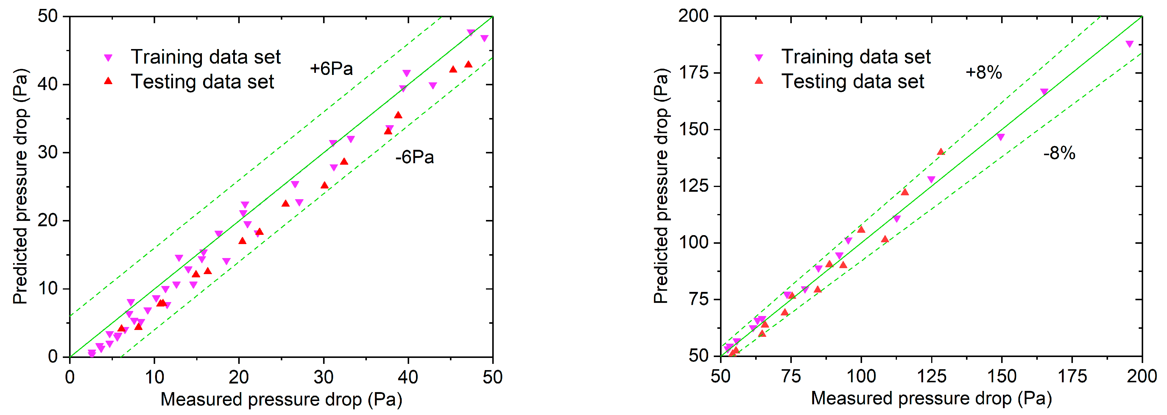
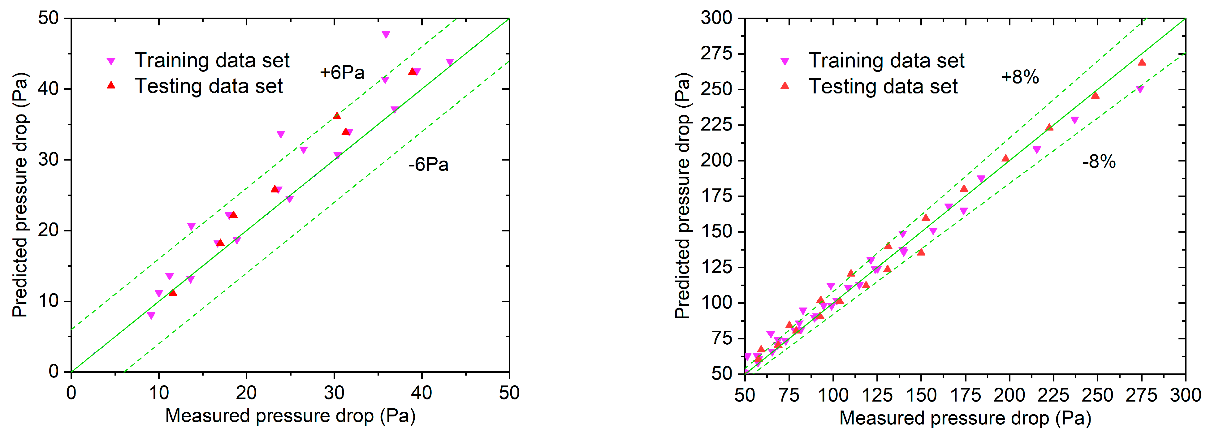
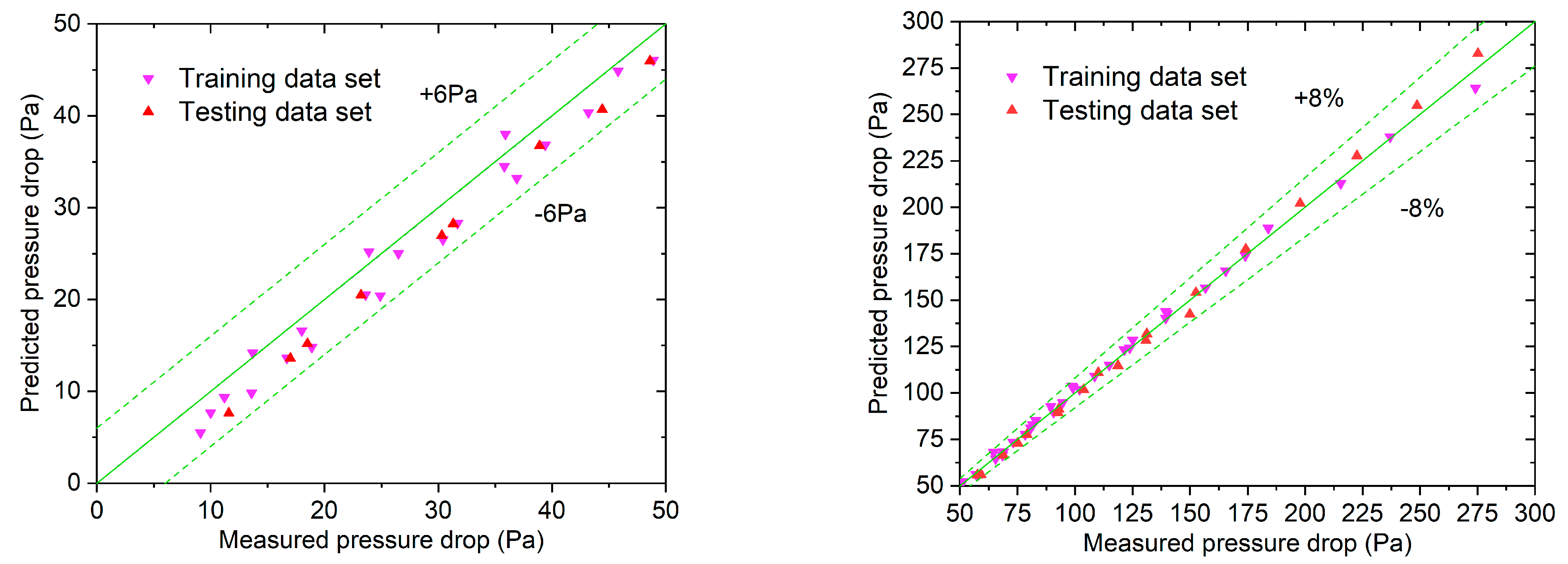
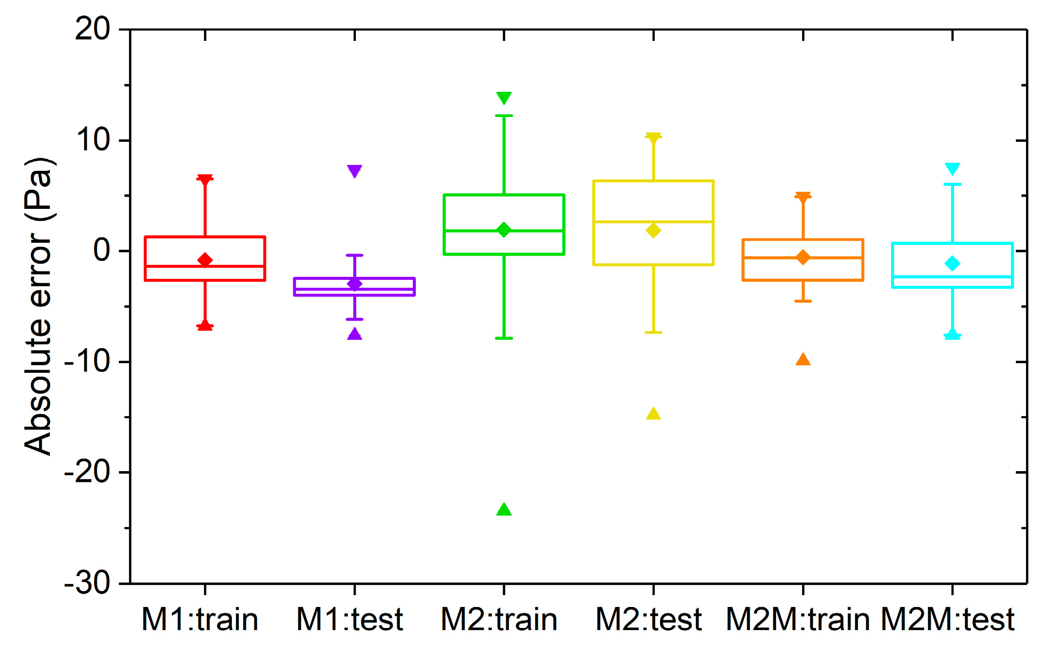
In the prediction process, the model is trained with the pressure drop data obtained from a series of experiments, which are called training data sets. The difference between the predicted and measured pressure drop results can be utilized to analyze the prediction accuracy of the model. In order to further validate the prediction accuracy of the model, the experimental data, which are called testing data sets, are obtained independently of the training sets. This part of the data can be used to independently validate the prediction accuracy of the model.

3. Results and Discussion

3.1. Experimental Results of Pressure Drop in Fibrous Core Materials

In this section, the pressure drop of the material was experimentally investigated. The impacts of varying the carbon content, the number of material layers, and the airflow velocity on material pressure drop were investigated. Figure 6 illustrates the variation of pressure drop with head-on air speed for different layers of substrate material.

Figure 6 shows that the pressure drop of the substrate material increased with the increase of the airflow velocity and the number of layers of the material, and the pressure drop did not vary linearly with the airflow velocity. For example, for the substrate material with 12 layers, the pressure drop increased from 40 Pa to 92 Pa when the airflow velocity increased from 0.4 m/s to 0.8 m/s, and it further increased to 156 Pa when the airflow velocity increased to 1.2 m/s. Figure 7 demonstrates the variation of pressure drop with airflow velocity of the tested material with different adsorption material amounts. The specific parameters of the four tested materials are shown in

Table 2. Test material parameters in Figure 7.

Test Material ID (4 Layers)	1	2	3	4
Layer number of material	4	4	4	4
Material width W (cm)	40	40	40	40
Material height H (cm)	40	40	40	40
Substrate material content (kg)	0.108	0.108	0.108	0.108
Total content (kg)	0.186	0.289	0.343	0.409

. The relative error of adsorption material amount of each layer material for the same material ID was measured to be within ±8% of the mean value. Test results showed that the adhesion amount of adsorption material has a large effect on the pressure drop. The higher the airflow velocity, the greater the influence of the adsorption material amount on the pressure drop. For example, the pressure drop of the material (ID:4) was about 2.6 times of that of the material (ID:1) when the airflow velocity was 1.4 m/s, while the pressure drop of the material (ID:4) was about 2.2 times of that of the material (ID:1) when the airflow velocity was 0.7 m/s. Test results show that when designing energy wheels and air cleaners with the studied material, the adsorption material amount of the material and the air flowrate should not be too high, as these can lead to excessive pressure drops of the devices and thus to high energy consumption of the fan.

Figure 8 shows the pressure drop of the tested material with different numbers of layers. The specific parameters of each layer of the tested material are shown in

Table 3. Test material parameters in Figure 8.

Layer ID (Single Layer)	1	2	3	4	5	6	7
Material width W (cm)	40	40	40	40	40	40	40
Material height H (cm)	40	40	40	40	40	40	40
Substrate material content (kg)	0.027	0.027	0.027	0.027	0.027	0.027	0.027
Total content (kg)	0.098	0.106	0.103	0.102	0.111	0.106	0.104

. Figure 8 shows that at a certain airflow velocity, the pressure drop increases with increasing numbers of layers, which shows that the thickness of the material is also an important design parameter of the device. For example, the pressure drop of the single-layer material was 57 Pa when the airflow velocity was 1.4 m/s, while the pressure drop of the 7-layer material was increased to 398 Pa.

3.2. Analysis of the Prediction Results

In this section, the total pressure drop of the material was predicted with the help of the method described in Figure 5, and the predicted results were analyzed. The pressure drop model of the substrate material was trained using the experimental data in Figure 6, while the pressure drop increase model was trained using the experimental data in Figure 7. Additional tests were conducted to verify the prediction accuracy of the model, and they were considered as testing data points. The test results are displayed in

Table 4. Testing data sets.

Data Point ID	$\mathit{u}\left(\mathbf{m}/\mathbf{s}\right)$	$\Delta {\mathit{p}}_{\mathit{i}}\left(\mathbf{P}\mathbf{a}\right)$	$\Delta {\mathit{p}}_{\mathit{t}}\left(\mathbf{P}\mathbf{a}\right)$	Data Point ID	$\mathit{u}\left(\mathbf{m}/\mathbf{s}\right)$	$\Delta {\mathit{p}}_{\mathit{i}}\left(\mathbf{P}\mathbf{a}\right)$	$\Delta {\mathit{p}}_{\mathit{t}}\left(\mathbf{P}\mathbf{a}\right)$
1	0.2	8.1	11.6	15	0.2	6.1	18.5
2	0.3	11	17	16	0.3	10.7	30.3
3	0.4	14.9	23.2	17	0.4	16.3	44.4
4	0.5	20.4	31.3	18	0.5	22.4	59.2
5	0.6	25.5	38.9	19	0.6	30.1	75.2
6	0.7	32.4	48.6	20	0.7	37.6	92.9
7	0.8	38.8	57.6	21	0.8	45.3	110.1
8	0.9	47.1	68.8	22	0.9	55.4	131.2
9	1.0	54.2	79.1	23	1.0	65.7	152.6
10	1.1	64.7	92.6	24	1.1	75.4	174.2
11	1.2	72.8	103.8	25	1.2	88.7	197.9
12	1.3	84.5	118.7	26	1.3	100	222.6
13	1.4	93.6	130.9	27	1.4	115.5	248.7
14	1.5	108.5	150	28	1.5	128.3	275.2

, and the parameters of the tested materials are listed in

Table 5. Test material parameters of testing data sets.

Data Point ID	1–14	15–28
Layer number of material	2	8
Material width W (cm)	40	40
Material height H (cm)	40	40
Substrate material content (kg)	0.054	0.216
Total content (kg)	0.204	0.622

. Considering the limited difference in material thickness for different amounts of carbon on the material, the number of layers was used to express the material thickness for the convenience of modeling, and the influence of carbon amount on material thickness was merged into other terms. For multilayer materials, $m_d$ was taken as the average value of this parameter for each layer of material. When training the nonlinear model, the Levenberg-Marquardt method [25] was used. After the model was built, the prediction results were obtained for both the training data points and the testing data points with the help of the built model. Figure 9 and Figure 10 show the comparison of the predicted and tested $\Delta p_i$ and $\Delta p_t$, respectively.

It can be seen from Figure 9 and Figure 10 that when the pressure drop is less than 50 Pa, the absolute error of prediction can be controlled within ±6 Pa for both training sets and testing sets. When the pressure drop is greater than 50 Pa, the relative error of prediction is less than ±8% for most data sets. These data show that the prediction accuracy of the model is acceptable, and it is much higher than that of the previous study on porous materials [6].

The root mean square error ($RMSE$) and mean absolute percentage error ($MAPE$) were used to analyze the prediction accuracy of the model. These two indicators were used because $RMSE$ can be used to reflect the absolute prediction error, and $MAPE$ can be used to indicate the relative prediction error, and they can provide a comprehensive picture of prediction accuracy. They can be calculated using the following equations:

$$RMSE=\sqrt{\frac{{{\displaystyle \sum }}_{i=1}^n{\left(x_{p,i}-x_{e,i}\right)}^2}{n}}$$

(13)

$$MAPE=\frac{1}{n}{{\displaystyle \sum }}_{i=1}^n\left|\frac{x_{p,i}-x_{e,i}}{x_{e,i}}\right|$$

(14)

Here, $x$ is the pressure drop value, and subscripts p and e represent the predicted pressure drop and the tested pressure drop, respectively. Since training sets and testing sets are independent data sets, it is better to analyze the predictions results of them separately. As a result, the $RMSE$ and $MAPE$ values of training sets and testing sets were calculated separately. The calculation results are listed in

Table 6. $RMSE$ and $MAPE$ values of the prediction model.

Parameters	$\Delta {\mathit{p}}_{\mathit{t}}$
$RMSE$ training sets	2.7 Pa
$RMSE$ testing sets	4.0 Pa
$MAPE$ training sets	5.2%
$MAPE$ testing sets	6.6%

.

The absolute error of the predicted pressure drop is defined by

$$AE=x_p-x_e$$

(15)

Table 6 shows that the $RMSE$ and $MAPE$ values of training sets for $\Delta p_t$ are less than 3 Pa and 6%, and the $RMSE$ values of testing sets are no more than 4 Pa and 7%.

3.3. Further Discussion of the Pressure Drop Prediction Method

The key idea of the method proposed in Section 2.3 is to divide the total pressure drop of the material into two separate parts for prediction. In an effort to simplify the prediction process, an alternative total pressure drop prediction method is proposed, and its prediction accuracy is compared with the accuracy of the method mentioned in Section 2.3. The method attempts to predict the total pressure drop directly on the basis of the substrate material pressure drop. First, the pressure drop prediction model of the substrate material is obtained using the method proposed in Section 2.3, after which the total pressure drop prediction model is directly established based on the pressure drop prediction model for the substrate material. In this way, the prediction process can be simplified.

Test results in Section 3.1 shows that the total pressure drop of the material increases with an increase in the amount of adsorption material, based on the substrate material pressure drop, and that the pressure drop rises with higher amounts of adsorption material. The total pressure drop model is simplified by multiplying the substrate material pressure drop model by a factor that contains the adsorption material amount. Consequently, the following total pressure drop prediction model is established:

$$\Delta p_t=(j_{1}u+j_2{u}^2)L^{j_3}{u}^{j_4}\left(1+k_1{m}_d{}^{k_2}\right)\left(1+k_3{m}_d{}^{k_4}\right)$$

(16)

Here, $j_i$s and $k_i$s are undetermined coefficients which can be obtained via regression.

To account for the potential difference in the impact of air velocity on the pressure drop characteristics of the substrate material and the material sprayed with adsorption materials, an additional term containing the air velocity is added in Equation (17). In this way, the relationship between airflow velocity and total pressure drop is determined through two regression processes. The modified prediction model of the total pressure drop can be expressed as follows:

$$\Delta p_t=(j_{1}u+j_2{u}^2)L^{j_3}{u}^{j_4}\left(1+k_1{m}_d{}^{k_2}\right)\left(1+k_3{m}_d{}^{k_4}\right)u^{k_5}$$

(17)

Using this method, the total pressure drop of the tested material can be predicted follow the steps below:

A.

Obtain the tested data for prediction ($u,L,m_d,\Delta p_s, \Delta p_t$).

B.

Train the substrate material pressure drop prediction model and obtain the coefficient $j_i$s.

C.

Calculate $\Delta p_s$ with the trained model.

D.

Train the total pressure drop prediction model and obtain the coefficient $k_i$s.

E.

Calculate the predicted $\Delta p_t$ with the trained model.

The above prediction process is depicted specifically in Figure 11.

The total pressure drop of the material was predicted using the method described in this Section. The training data points and the testing data points are the same as those used in Section 3.2. To study the effect of model modification on the improvement of prediction accuracy, the total pressure drop was predicted using Equations (16) and (17), respectively. The prediction results of $\Delta p_t$ using Equations (16) and (17), are shown in Figure 12 and Figure 13, respectively, and

Table 7. $RMSE$ and $MAPE$ values of the method proposed in Section 3.3.

Parameters	$\Delta {\mathit{p}}_{\mathit{t}}$	$\Delta {\mathit{p}}_{\mathit{t}}$ (After Modification)
$RMSE$ training sets	6.3 Pa	2.8 Pa
$RMSE$ testing sets	6.0 Pa	3.6 Pa
$MAPE$ training sets	8.2%	5.9%
$MAPE$ testing sets	7.1%	6.1%

shows the calculated results of the accuracy indices of the method proposed in this section using Equations (16) and (17).

It can be seen from Figure 12 and Figure 13 that the prediction accuracy of the method proposed in this section using Equation (17) was obviously higher than that using Equation (16). Moreover, Table 7 shows that after integrating the modified model, as expressed by Equation (17), the $RMSE$ and $MAPE$ values of both training sets and testing sets decreased significantly. For example, the $MAPE$ value of training sets decreased from 8.2% to 5.9%, and the $MAPE$ value of testing sets decreased from 7.1% to 6.1%. This indicates that determining the relationship between airflow velocity and total pressure drop through two regression processes helps to mitigate prediction errors effectively. Figure 10 and Figure 13 demonstrate that the proposed method, utilizing the modified model, exhibits a similar level of prediction accuracy as that in Section 2.3. For example, when the pressure drop is below 50 Pa, the absolute prediction error can be controlled within ±6 Pa, and when the pressure drop is greater than 50 Pa, the relative prediction error is within ±8% for most data sets.

Figure 14 depicts the absolute prediction error of two distinct prediction methods. Figure 14 clearly illustrates that the range of absolute prediction error using Equation (17) is noticeably smaller than that using Equation (16). The absolute prediction error of testing sets using Equation (17) ranges from −7.6 Pa to 7.6 Pa, while that using Equation (16) ranges from −14.8 Pa to 10.3 Pa. The primary advantage of this method is its reduced number of prediction steps compared to that in Section 2.3. However, it should be noted that the predicted total pressure drop in this method is based on the predicted results of the substrate material pressure drop. Consequently, this approach is more reliant on the predicted data of the substrate material pressure drop.

4. Conclusions and Future Work

This study investigated the pressure drop in a fiber–powder composite material. Referring to the fiber–powder structure of the material, two pressure drop prediction methods with different prediction strategies were proposed, and their prediction accuracies were analyzed. Both methods take into account the differences in pressure drop characteristics between the substrate and composite materials. As verified by experimental data, both proposed methods demonstrated acceptable prediction results. Specifically, the absolute prediction error of them was within ±6 Pa when the pressure was below 50 Pa, and the relative prediction error was within ±8% for the majority of data points when the pressure exceeded 50 Pa. Each method has its advantages; the first proposed method is less reliant on the predicted results of the substrate material pressure drop, while the second proposed method involves fewer prediction steps.

The proposed prediction methods were validated within certain ranges. For example, the airflow velocity ranged from 0.2 m/s to 1.5 m/s, and the number of material layers ranged from 2 layers to 8 layers. In the future, more test data will be used to further verify the model and to explore whether its applicability can be expanded. Prediction results in Section 3.3 show that determining the relationship between airflow velocity and total pressure drop through two steps instead of one step helps to reduce prediction errors, and as a result, more studies on the optimization of the prediction process can be conducted in the future to further improve the prediction method.