A Facility’s Energy Demand Analysis for Different Building Functions

Abstract

A more accurate determination of energy demands for buildings is of utmost importance for estimating future energy demands. This article presents two novel ideas that have the potential to contribute to a more precise determination of expected energy demands. The first idea involves accounting for a building’s function more thoroughly, which enables the determination of different energy demands for two or more identical buildings, depending on their respective usage functions. According to a case study, the heating energy demand can be up to twice as high in a commercial facility compared with a residential building. Similarly, the cooling energy requirement can also differ. The second idea concerns determining the heating degree day (HDD) and cooling degree day (CDD) values from the daily minimum and maximum temperatures. This idea may be relevant when few instantaneous values are available for the daily mean temperature. According to the case study, the calculated values from the daily minimum and maximum temperatures follow the HDD and CDD values specified from the daily mean temperature. However, the difference is less than 2% for the heating season and higher for the cooling season. Therefore, further research is required to refine the constants in the cooling equation.

1. Introduction

Human activities contribute significantly to global warming, which is now widely accepted as a reality. To lessen this contribution, the main energy consumers must be examined. Building heating accounts for the biggest share of energy consumption, accounting for 12% of global energy usage and 13% (4.3 Gt) of CO₂ emissions [1]. In Hungary, heating energy consumption accounts for 70% of the total energy consumption in residential buildings [2]. In comparison, cooling accounts for only 2% of global energy usage and 3% of CO₂ emissions (1 Gt) [1]. The ratios can vary between countries due to differences in applicable comfort categories [3] and variable radiative heat gains [4]. Energy requirements can be reduced through various methods, such as the insulation of buildings [5,6] and mechanical systems [7,8] or through thoughtful operational strategies [9]. Previous research has shown that regulatory policies are the most effective means of reducing energy consumption in residential heating, highlighting the need for increased attention to this area for successful energy reduction [10]. Accurate estimates of the energy demands of buildings are required, taking into account the precise values of various factors [11,12]. The energy consumption of buildings is highly dependent on local meteorological conditions [13], regardless of the energy efficiency of individual buildings [14]. Therefore, precise determination of the energy demands of buildings and consideration of environmental factors are necessary for practicable regulations.

Research on estimating the future energy consumption of buildings has been and continues to be conducted worldwide. Ciancio et al. [15] analyzed energy consumption trends in different European cities, while Morakinyo et al. [16] presented research on Hong Kong’s urban energy demand. Cao et al. [13] emphasized the need for a general analysis of temporal changes in building energy demand and extrapolated data from the past two decades to present realistic scenarios for the future. While these studies primarily focus on metropolitan regions, it is crucial to highlight that a significant percentage of the population in Hungary lives in small-town environments (5000–200,000 inhabitants). Therefore, these results should be approached with caution [17].

Several methods are available for the analysis and prediction of energy consumption by heating and cooling season, among which the degree-day approach [18] stands out, being used for the estimation and analysis of the weather-related energy consumption of buildings [19,20,21]. It is generally accepted that seasonal energy consumption depends on, among other things, heating degree days (HDDs) and cooling degree days (CDDs), respectively [22,23]. European legislation often uses the HDD value to characterize the energy performance of buildings, for example, in the EU Directive on the Energy Performance of Buildings [24].

To calculate HDD and CDD values, it is necessary to sum the positive temperature differences over a certain period between the indoor and outdoor air temperatures [25,26]. To determine the length of this period, a base temperature is necessary, which is the external temperature at which further cooling or heating is not needed to maintain a designed internal environment [11,27]. In other words, it can also be referred to as the balance-point temperature, because this is the external temperature when heat gain and heat loss are equal [27,28]. The value of the balance-point temperature, or base temperature, varies depending on several factors, including the thermal characteristics of the building [29]. However, the only locally dependent parameter in the applied approach is the balance-point temperature [30,31]. It is important to emphasize that choosing the correct balance-point temperature is essential for the accurate prediction of a building’s energy consumption [32].

For each country, a different standard is often given for buildings’ balance-point temperature. For heating balance-point temperature, the European standard EN ISO 15927-6 recommends 12.0 °C [33], while Carbon Trust (UK) suggests 15.5 °C [34], and ASHRAE recommends 18.3 °C. The daily heat gain is generally higher during the cooling season than during the heating season. As a result, in the case of CDDs, the balance-point temperature without ventilation might be lower than in the case of HDDs. For this reason, ASHRAE, for example, also uses 10.0 °C for the cooling balance-point temperature in addition to 18.3 °C [35]. Unfortunately, these standards do not consider a building’s function or user habits and often prescribe the same base-point temperature all year round (i.e., ignore the differences between heating and cooling seasons). As a result, the standard base-point temperatures often deviate from the balance-point temperatures used in research. Azevedo et al. [30] reviewed the balance-point temperatures associated with the degree-day method and found significant differences among the balance-point temperatures used, even within the same country. The average balance-point temperatures reported in their literature review were 18.1 °C (heating season) and 22.0 °C (cooling season).

The energy consumption of a building is influenced not only by the external temperature but also by various other factors. These factors encompass the thermal properties of the building, including materials, exterior cladding systems, and types of curtain walls. Furthermore, building management systems (BMSs) and automated building systems (ABSs) should also be considered. Moreover, energy consumption can also be influenced by possible renovations of the building or even user behavior [36,37].

After summarizing the energy-demand estimation using the degree-day method, two novel ideas are presented in this article. One concept proposes the incorporation of a new factor to better account for the impact of a building’s function on its energy demand. This factor aims to enhance the accuracy of energy-demand assessments by considering the specific usage functions of the building. The other concept focuses on determining the HDD and CDD values based on the daily maximum and minimum temperatures. It understands that the daily mean temperature is not independent of the daily minimum and maximum temperatures, and as a result, the derived degree-day values are interconnected. Subsequently, we attempt to demonstrate the usability of the two ideas through a case study. In the case study, their usability is investigated by varying two parameters. One is the internal temperature (±3 °C), and the other is the air change rate (between 0 and 9 1/h). Finally, in the discussion, the relevance of the correlations given to determine the HDD and CDD values in other cities is investigated to find the impact of varying these two parameters on the accuracy of these correlations.

2. Theoretical Background

Describing the varying external temperature can be applied to the daily mean, the daily maximum, and the daily minimum temperatures, too. If these temperatures and the days of the year are arranged such that the number of days for each temperature value is related to that value, a curve known as the degree-day curve is obtained. The degree-day curve for Debrecen (Hungary) based on the years 1991–2020 is shown in Figure 1a. The Hungarian Meteorological Service (OMSZ) took the necessary measurements for the graph.

The degree-day curve can be used to determine the degree-day values (Figure 1b) given the knowledge of the internal temperature and the heating/cooling balance-point temperature. The heating (“T_B,H”) and cooling balance-point temperatures (“T_B,C”) can be determined using the following equation [26]:

$$T_B=T_i-\frac{{\dot{Q}}_s+{\dot{Q}}_i}{H_{tr}+H_{ve}}\hspace{1em};\hspace{1em}\left[K\right]$$

(1)

where “T_B” is the balance-point temperature (for the heating or cooling season), in [K]; “T_i” is the internal set-point temperature for the heating or cooling season, in [K]; “Q_s” is the daily mean value of solar gains, in [W]; “Q_i” is the daily mean value of internal gains, in [W]; “H_tr” is the heat-loss coefficient for transmission [W/K]; and “H_ve” is the heat-loss coefficient for ventilation [W/K].

The mathematical description of the heating and cooling degree-day value is as follows [26]:

$$HDD=\underset{j=1}{\overset{N_{heating}}{\int }}\left(T_i-{\overline{T}}_{ej}\right)·dt\hspace{1em};\hspace{1em}\left[hK\right]$$

(2)

$$CDD=\underset{j=1}{\overset{N_{cooling}}{\int }}\left({\overline{T}}_{ej}-T_i\right)·dt\hspace{1em};\hspace{1em}\left[hK\right]$$

(3)

where “HDD” is the degree-day value of the heating season, in [hK]; “CDD” is the degree-day value of the cooling season, in [hK]; “T_ej” is the mean outdoor temperature of the “j” heating or cooling day, in K; and “N” is the number of days in a heating or cooling season, in [–].

The heating and cooling energy demand of the building can be determined using the degree-day values [26]:

$$E_H=\left(H_{tr}+H_{ve}\right)·HDD=\left(H_{tr}+H_{ve}\right)·\underset{j=1}{\overset{N_{heating}}{\int }}\left(T_i-{\overline{T}}_{ej}\right)·dt\hspace{1em};\hspace{1em}\left[Wh\right]$$

(4)

$$E_C=\left(H_{tr}+H_{ve}\right)·CDD=\left(H_{tr}+H_{ve}\right)·\underset{j=1}{\overset{N_{cooling}}{\int }}\left({\overline{T}}_{ej}-T_i\right)·dt\hspace{1em};\hspace{1em}\left[Wh\right]$$

(5)

where “E_H” is the building energy demand for the heating season, [Wh], and “E_C” is the building energy demand for the cooling season, [Wh].

3. Results

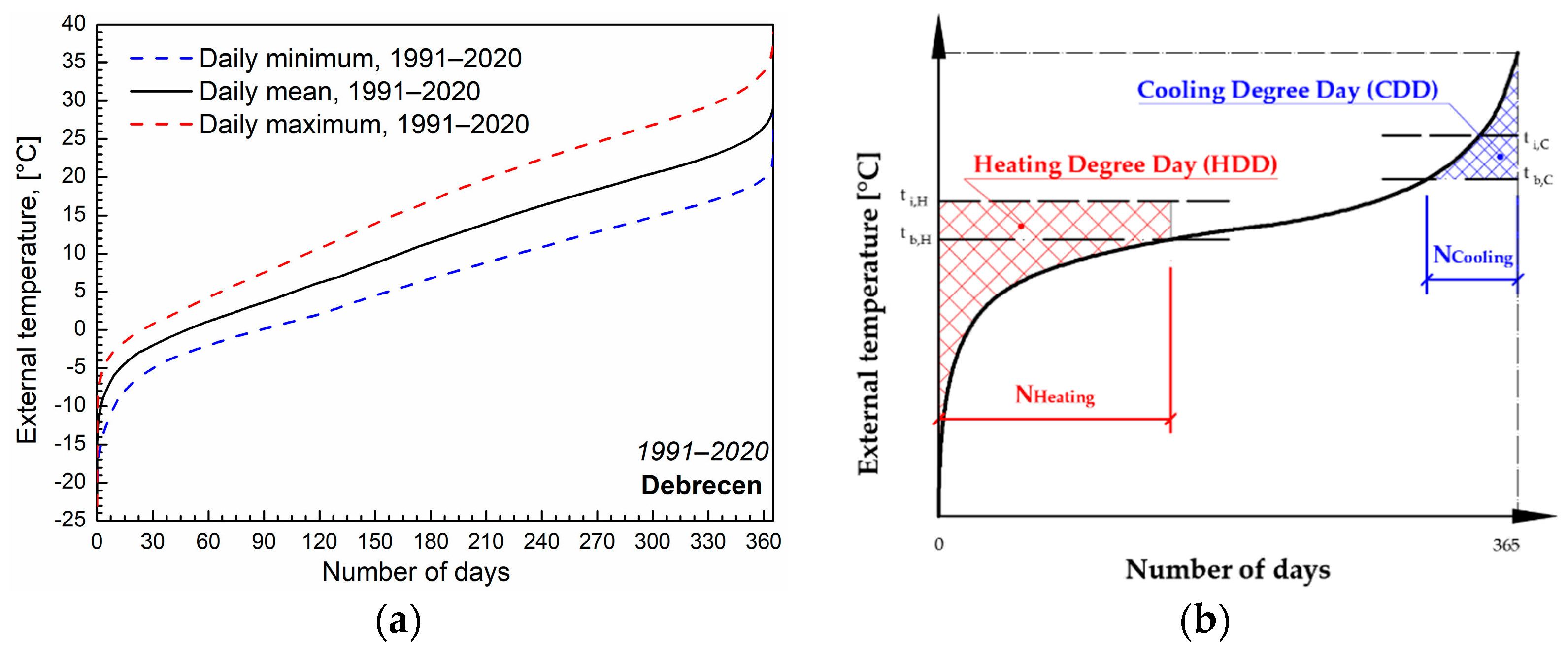
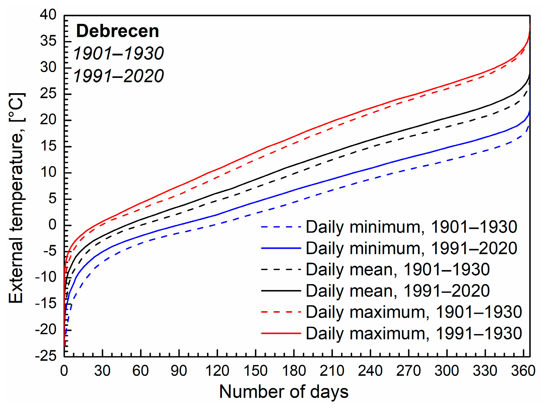
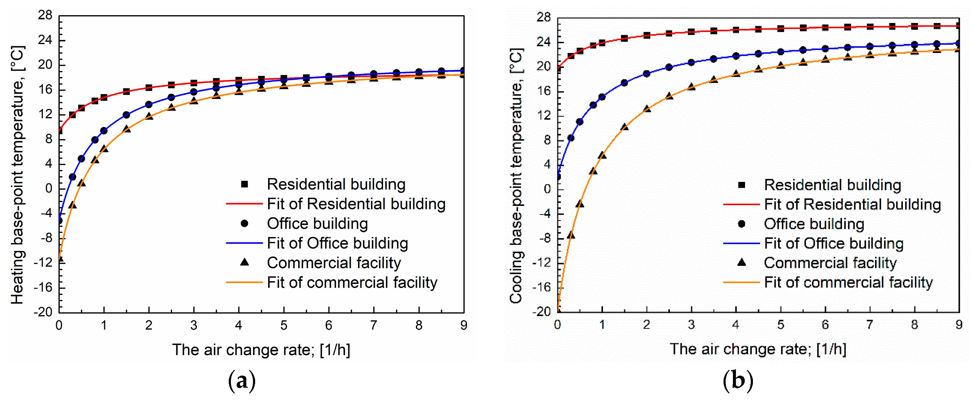
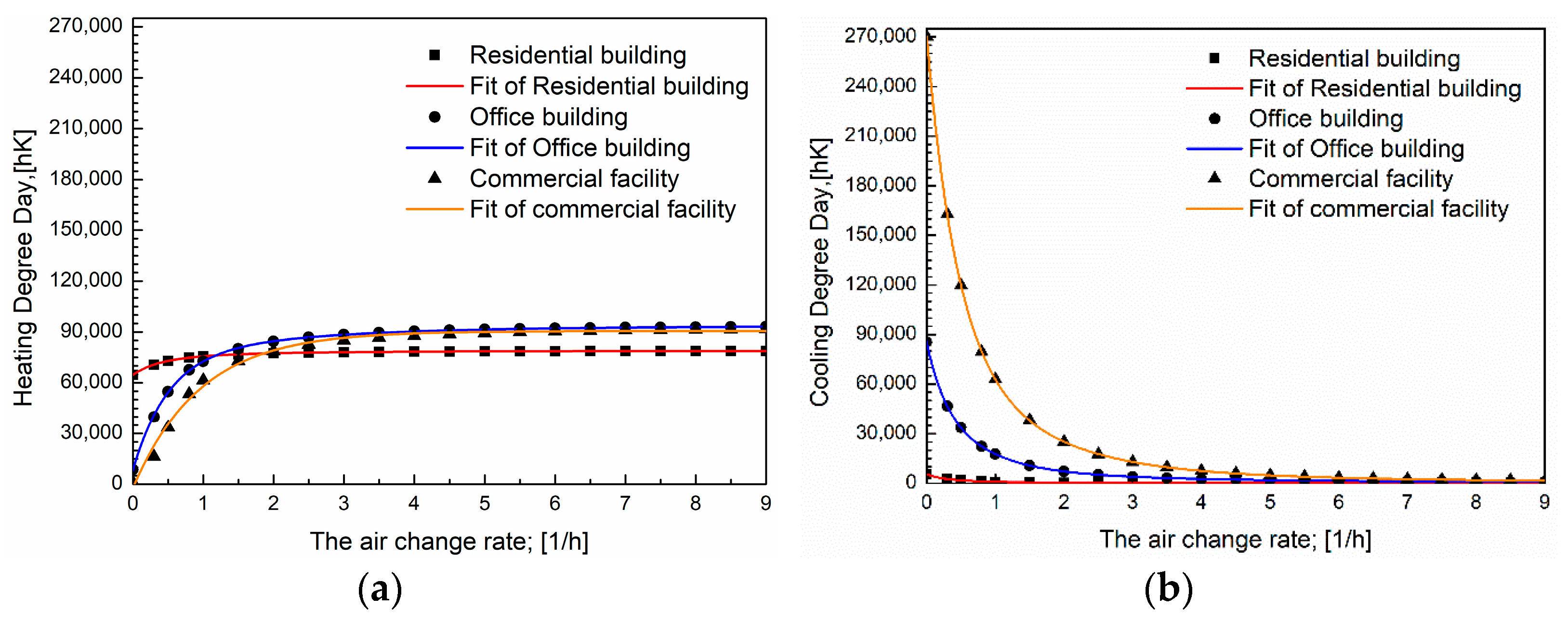
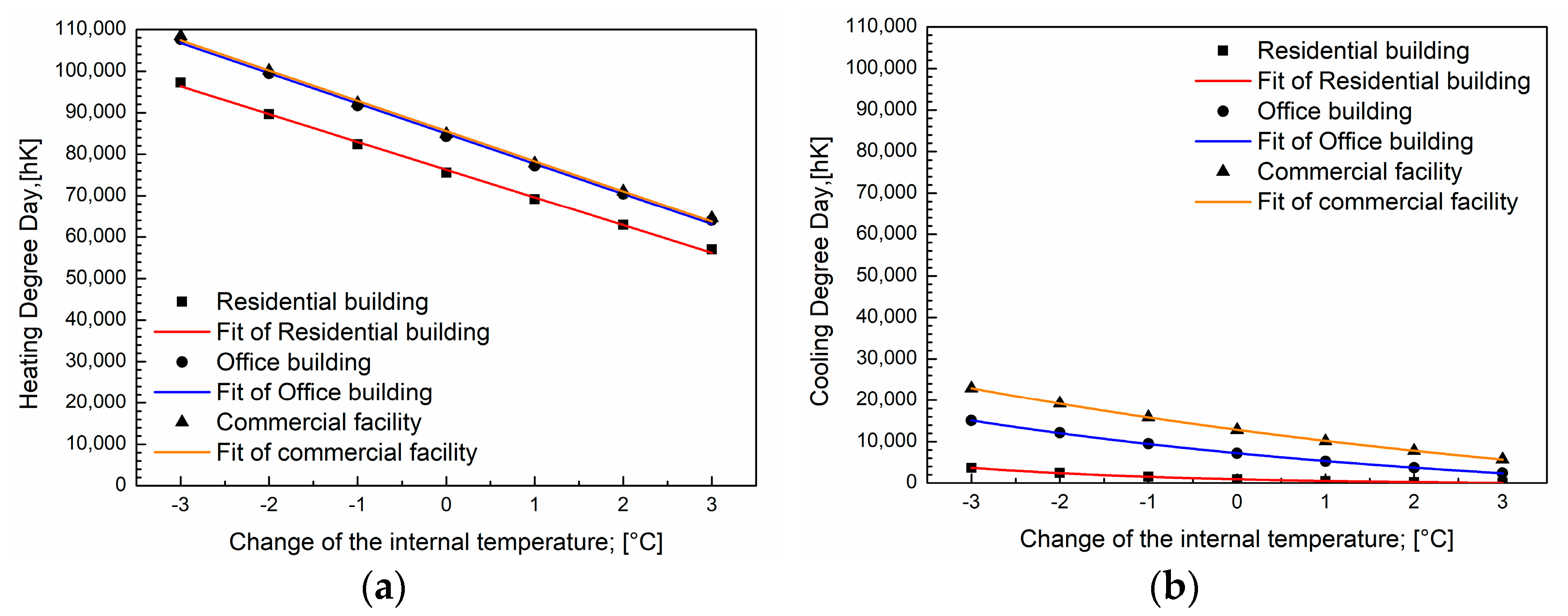
3.1. Novel Determination of Degree-Day Values

The daily minimum, the daily mean, and the daily maximum temperatures between 1901–1930 and 1991–2020 were compared in Debrecen (Figure 2):

Between these two periods, there was an average increase of 2.16 °C in the daily minimum temperature, 1.49 °C in the daily mean temperature, and 1.14 °C in the daily maximum temperature. It seems advisable to develop a method by which the different rates of increase in the extreme values can be calculated.

Unfortunately, the daily minimum and maximum temperatures are momentary values. In contrast, the daily mean temperatures were calculated from multiple temperature readings; thus, generally, they provide a more accurate basis for calculating energy demands. However, if only a few or exactly two (the daily minimum and maximum) temperatures are known, then the calculations become imprecise. This article aims to explore a solution for this particular scenario.

The proposed solution is based on the understanding that the daily minimum and maximum temperatures are not independent of the daily mean temperature. Consequently, the degree-day values derived from them are also interdependent. It has been determined that the degree-day values obtained from the daily minimum temperature (“HDD_min” or “CDD_min”) and the daily maximum temperature (“HDD_max” or “CDD_max”) can be utilized as approximations for the degree-day values derived from the daily mean temperature (“HDD” or “CDD”). Various equations were tested using the “Nonlinear Curve Fit” feature in OriginPro to describe their relationships. For heating cases, it was found that the most accurate approximation is obtained by calculating the arithmetic and harmonic means of “HDD_min” and “HDD_max”, followed by taking the arithmetic mean of these two means. Therefore, the following equation can be used for heating:

$$HDD=\frac{{HDD}_{max}+{HDD}_{min}}{4}+\frac{1}{\frac{1}{H{DD}_{max}}+\frac{1}{{HDD}_{min}}}\hspace{1em};\hspace{1em}\left[hK\right]$$

(6)

where “HDD_max” is the degree-day value of the heating season from the daily maximum temperature, in [hK], and “HDD_min” is the degree-day value of the heating season from the daily minimum temperature, in [hK].

Determining the cooling degree-day value was more problematic. Finally, the most successful solution was to take the arithmetic average of two approximate equations. In one of the equations, the degree-day value derived only from the daily minimum temperature was used, while in the other, the degree-day value derived only from the daily maximum temperature was applied as a variable. Therefore, the cooling case is:

$$CDD=\left[a·{\left({CDD}_{max}+b\right)}^c\right]+\left[d+e·{{CDD}_{min}}^f\right]\hspace{1em};\hspace{1em}\left[hK\right]$$

(7)

where “CDD_max” is the degree-day value of the cooling season from the daily maximum temperature, in [hK], and “CDD_min” is the degree-day value of the cooling season from the daily minimum temperature, in [hK]. “a”–“f” are constants.

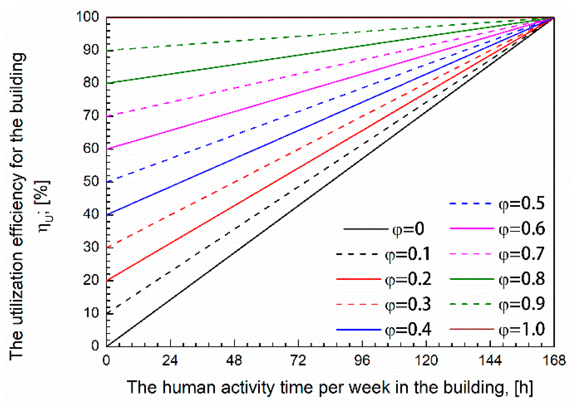
3.2. Considering the Building Function with the Utilization Efficiency for a Building

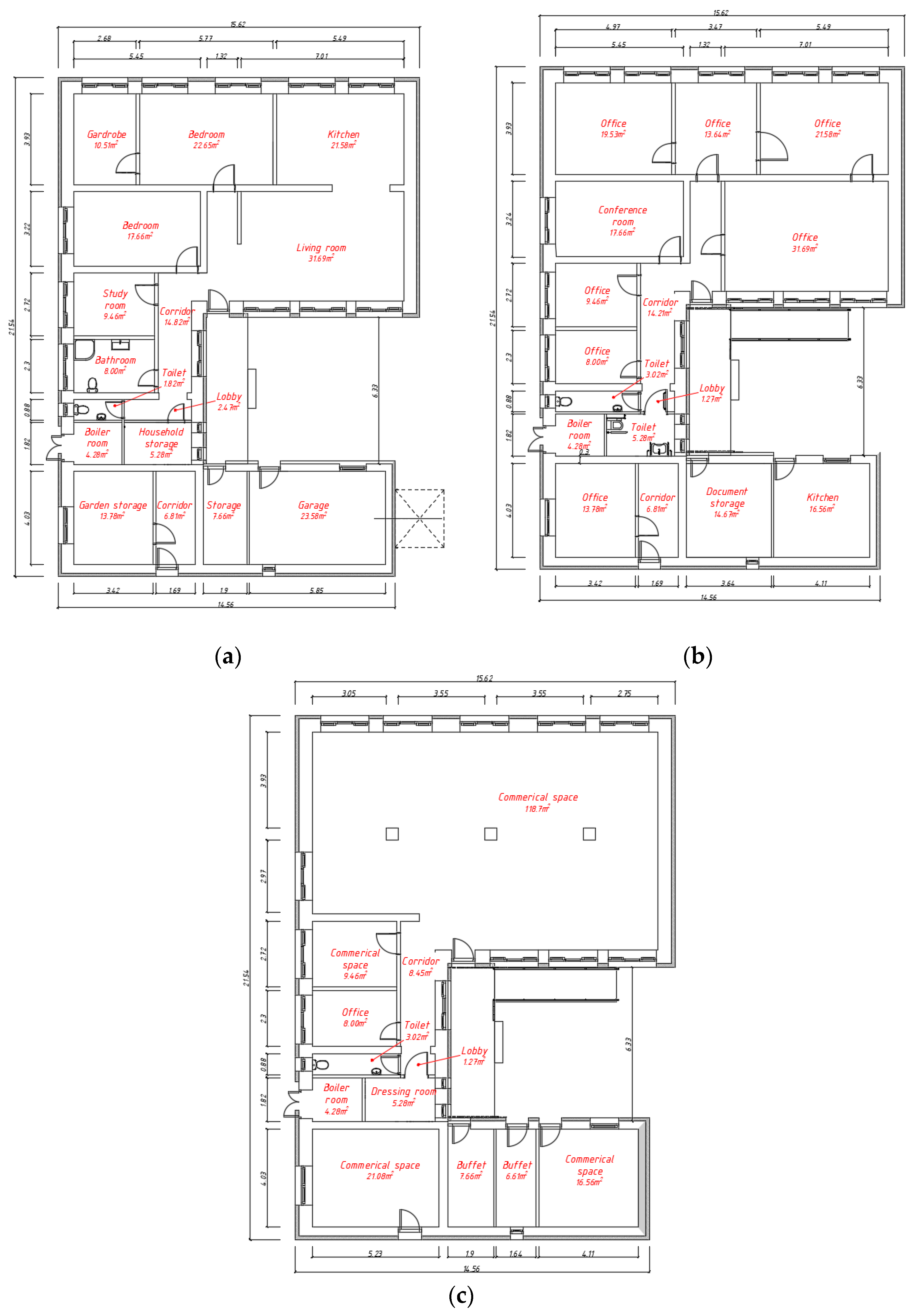
From the perspective of human usage, the operation of HVAC systems in a building can be divided into two distinct periods: activity and passivity. The activity period is primarily determined by the elapsed time, while the passivity period depends on the extent to which the HVAC system can be back-regulated compared with the activity period. By considering the combined duration of the passivity period, which is corrected by the ratio of back-regulation, and the activity period, a latent time that characterizes the system’s functioning within a specified time frame can be calculated. Relating this latent time to the investigated period, a more comprehensive efficiency factor may be given. Although it is feasible to examine several time intervals, focusing on a weekly period proves to be more practical. By adopting this approach, a novel efficiency factor, namely the utilization efficiency of a building, can be introduced:

$${\eta }_U=\frac{A+\left(168-A\right)·\overline{\phi }}{168}·100\hspace{1em};\hspace{1em}\left[\%\right]$$

(8)

where “η_U” is the utilization efficiency for a building (heating or cooling mode), in [%]; “A” is the human activity time per week in the building (heating or cooling mode), in [h]; and “ $\overline{\phi }$” is the passivity operating ratio (heating or cooling mode), in [-].

The human activity time per week can vary widely, ranging from 0 h (for example, in a vacant vacation house) to 168 h (for example, in 24 h shops). Hence, the utilization efficiency value can change from “100∙$\overline{\phi }$” to “100%”. When determining the passivity operating ratio, it is essential to consider the differences between heating and cooling HVAC systems and the variations in human utilization of these systems. Therefore, it is advisable to provide distinct utilization efficiency values for a building during the heating (“η_U,H”) and cooling (“η_U,C”) seasons. The following diagram (Figure 3) can also be used to determine utilization efficiency:

The heating and cooling energy demand, corrected by the utilization efficiency for a building, is:

$$E_H=\frac{{\eta }_{U,H}}{100}·\left(H_{tr}+H_{ve}\right)·HDD\hspace{1em};\hspace{1em}\left[Wh\right]$$

(9)

$$E_C=\frac{{\eta }_{U,C}}{100}·\left(H_{tr}+H_{ve}\right)·CDD\hspace{1em};\hspace{1em}\left[Wh\right]$$

(10)

where “η_U,H” is the utilization efficiency for the building (heating mode), in [%], and “η_U,C” is the utilization efficiency for the building (cooling mode), in [%].

4. Case Study

4.1. Background to the Investigation

In a small town near Debrecen, the energy demand of a newly built (currently still hypothetical) building is investigated from two viewpoints. These two aspects are the impacts of the building functions and the internal temperature change.

The building has the potential for several functions, including residential, municipal office, and commercial (e.g., food store) purposes, all of which are explored. Additionally, the study investigates the changes in the building’s energy demand resulting from implementing the European Union’s recommendations for reduced internal air temperatures during the heating season and elevated temperatures during the cooling season. Additionally, the study analyzes the differences in the heating and cooling degree-day values if calculated using the daily minimum and maximum temperatures.

The building has a floor area of 201.9 m², and its structures comply with Hungarian Regulation 7/2006 on the energy performance of buildings. The examined building has walls made of brick. The external walls are 50 cm thick, the internal load-bearing walls are 30 cm, and the partition walls are 10 cm. However, the windows are plastic. Due to the different functions, the interior layouts of the building differs from each other (Figure 4).

The indoor air quality of the building is affected by various factors, including the number of occupants and their activities, which influence the demand for fresh air. The different air change rates can be used to consider this demand. The balance-point temperatures for heating (Figure 5a) and cooling (Figure 5b) are changed exponentially (R² = 1) as a function of the air change rate. During the investigations, it was assumed that the value of the air change rate could occur between 0 [1/h] (no-use state) and 9 [1/h] (multi-facade, continuous artificial ventilation).

During the investigations, nominal air change rates (“n_nom”) of 1 [1/h] for a residential building, 2 [1/h] for an office building, and 3 [1/h] for a commercial facility were considered. These air change rate values were determined to be capable of adequately meeting the fresh-air demand of each building’s function.

The further data of the building are presented in

Table 1. The main data of the examined building.

Nomination	Symbol, [Unit]	Residential Building	Office Building	Commercial Facility
A/V ratio	A/V,	1.144	1.142	1.131
	[m2/m3]
Heat demand (EN 12831)	${\dot{Q}}_{\mathrm{HD}}$, [W]	10,113	17,377	23,572
Heat loss, from heat demand	${\dot{Q}}_{\mathrm{loss}}$, [W]	11,649	18,892	26,780
Heat loads (MSZ 04140)	${\dot{Q}}_{\mathrm{HL}}$, [W]	1986	8291	9082
Air change rate	nnom, [1/h]	1.0	2.0	3.0
The heat-loss coefficient for ventilation	Hve, [W/K]	185.45	367.5	577.12
The heat-loss coefficient for transmission	Htr, [W/K]	154.17	151.51	161.52
Indoor air temperature during the heating season	Ti,C, [°C]	19.3	21.4	21.3
Balance-point temperature during the heating season	TB,H, [°C]	14.8	13.66	14.17
Indoor air temperature during the cooling season	Ti,C, [°C]	27.37	25.86	26.9
Balance-point temperature during the cooling season	TB,C, [°C]	23.93	18.93	16.68

:

The internal partition walls also vary depending on the function of the building (e.g., a food store requires a large contiguous area). Due to these rearrangements, there will be minimal differences in the heat-loss coefficient for transmission and the A/V ratio value. Depending on the use, different air temperatures develop in each room, as the applicable Hungarian standards (e.g., MSZ 24140) prescribe different internal air temperatures based on the function. According to this standard, a residential building has fewer cooled spaces than an office or a commercial facility.

The daily minimum, maximum, and mean temperature values were measured by the Hungarian Meteorological Service (OMSZ). The observations were taken at 07:00, 13:00, and 19:00 h, while the nocturnal 01:00 h data were read from a thermograph. The times were in Central European Time (CET). The daily mean temperature was calculated as the average of the four readings. The maximum and minimum thermometers, too, were read at 07:00 and 19:00 h. The daily maximum temperature was the higher value between the two maximum temperatures, while the daily minimum temperature was the lower value between the two minimum temperatures.

The temperature values for 1991–2020 measured near Debrecen were used during the investigation.

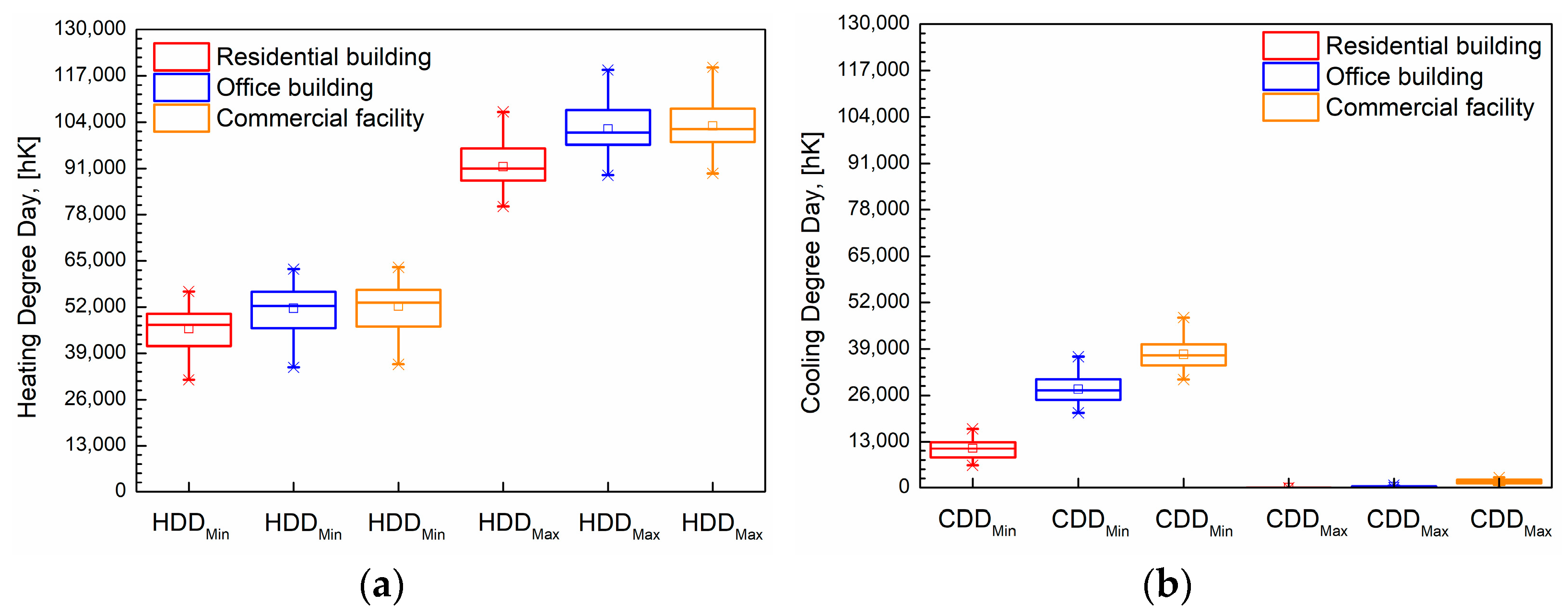
4.2. Calculating the Cooling and Heating Degree Days

Figure 6 displays the average degree-day values calculated from the daily mean temperature between 1991 and 2020 as a function of air change for the three examined building functions. The internal air temperatures are the standard temperatures (from MSZ 24140); thus, the changes are zero (∆t_i = 0 °C).

Based on the figure, both the heating degree day (R² > 0.99043) and the cooling degree day (R² > 0.99997) change exponentially as a function of the air change rate.

Figure 7 shows the average degree-day values calculated from the daily mean temperature between 1991 and 2020 as a function of the indoor temperature for the three examined building functions (n = n_nom).

Based on the figure, the heating degree day changes linearly (R² > 0.99759), while the cooling degree day changes exponentially (R² > 0.99905) as a function of the internal temperature. Interestingly, the curves for the office and the commercial building functions almost overlap. This similarity is because, for these two building functions, the difference between the internal temperature and the balance-point temperature is nearly the same (7.74 °C and 7.13 °C, respectively), while for the residential building, this value is 4.5 °C.

The degree-day values calculated from the daily minimum and maximum temperatures, determined using Equations (6) and (7), are compared with these values.

The calculated degree-day values from the daily minimum and maximum temperatures measured from 1991 to 2020 are shown in Figure 8 (Δt_i = 0 °C).

The values of the constants a−f appearing need to be determined using Equation (7). The values in

Table 2. The values of the constants used in Equation (7).

a	b	c	d	e	f
589.28	0.06461	0.3277	(−416.033)	0.000353	1.593

were optimized for the Debrecen data (1991–2020; all three building functions; Δt_i = ±3 °C) using the built-in Solver subroutine “GRG Nonlinear” in Microsoft Excel.

Figure 9 shows the deviation in determining heating and cooling degree days in the average of the 30 years studied when using Equations (6) and (7) instead of starting from the daily mean temperatures. (The nominal values of the heating and cooling degree days were determined from the daily mean temperatures.)

Based on Figure 9, in the heating case, the value is always smaller than the nominal but not higher than 1.5%. In the cooling season, higher deviations can occur, up to a difference of 9.4%. This value can be misleading, as the cooling degree-day value is much smaller than the heating degree-day value. Therefore, the extent of the deviation in [hK] was also examined.

The deviations from the nominal values of the heating and cooling degree days using each year’s data and applying Equations (6) and (7) for Δt_i = 0 °C are investigated in Figure 10.

Based on Figure 10a, the difference in the heating season was similar for each building function. For the residential building, the deviation was between +3979 and (−3600) hK; for the office, it was between +5051 and (−4588) hK; and for the commercial building function, it was between +4895 and (−4210) hK. In the cooling mode (Figure 10b), these deviations were also similar for each building function, but were significantly less than in the heating mode. For the residential building, the divergence ranged between +1410 and (−500) hK; for the office, it was between +1498 and (−1379) hK; and for the commercial facility, it was between +1512 and (−1883) hK.

4.3. The Determination of Energy Demand Takes into Account the Utilization Efficiency

The utilization efficiency for the three building functions examined can be calculated using Figure 3. But, their exact values are influenced by numerous factors, including owner expectations and local lifestyle. Applying this diagram, the “A” and “$\overline{\phi }$” must be determined. Both values can be specified precisely by the owner or the user as requirements. Without such specifications, only approximations can be used, for example, based on observations made by local HVAC system designers. In this additional case study, the only way can be to proceed. Based on the designed experience of the author (Bodó, B.) in Hungary, weekly activity time in residential buildings can range between 80 and 140 h, in offices between 40 and 72 h, and in commercial facilities between 40 and 100 h in rural small towns. The passive operational factor during the heating season may range between 70 and 100% in residential buildings, 70 and 100% in offices, and 40 and 70% in commercial facilities. During the cooling season, this factor may range between 0 and 50% in residential buildings, 0 and 70% in offices, and 0–80% in commercial facilities. As can be seen, the values can vary widely. This study considers the reasonably expected values, as shown in

Table 3. The utilization efficiency for the three building functions examined.

		A, [h]	$\overline{\mathit{\phi }}$, [-]	ηU, [%]
Heating season	Residential building	98	0.80	91.67
	Office building	45	0.70	78.04
	Commercial facility	66	0.70	81.79
Cooling season	Residential building	35	0.00	20.83
	Office building	45	0.30	48.75
	Commercial facility	66	0.00	39.29

.

The building’s heating energy demand can be determined using Equation (9), while its cooling energy demand can be calculated using Equation (10). The Figure 10 illustrates the impact of the air change rate on this heating and cooling energy (∆t_i = 0 °C). Figure 11a,c show the energy demand determined by the degree days from the daily mean temperature, while Figure 11b,d provide the energy demand calculated using the degree days from Equations (6) and (7).

The best fit for the heating energy demand was obtained with exponential fitting, both with the daily mean temperature (R² > 0.99973) and for the energy demand determined using Equation (6) (R² > 0.99982). The linear approximation was similar too, but resulted in a slightly worse fit (R² > 0.99861 and R² > 0.99866). The cooling degree day also exhibited an exponential trend as a function of the air change rate, both with the daily mean temperature (R² > 0.99695) and for the energy demand determined using Equation (7) (R² > 0.99875).

When determining the heating energy demand using Equation (6), higher deviations from the energy demand were obtained as determined with the daily mean temperature as the air change rate increased, which could be up to 2350 kWh (for the office building and n = 9 [1/h]). In the cooling season, on the other hand, the opposite occurred, with the highest deviations observed at low air change rates, where the highest divergence was 2484 kWh (for the commercial facility and n = 0.5 [1/h]).

The annual heating and cooling energy demand for the three building functions is shown in Figure 12 as a function of changing internal temperatures (for n = n_nom). Figure 12a,c show the energy demand determined by the degree days from the daily mean temperature. Figure 12b,d provide the energy demand calculated by degree days from Equations (6) and (7), respectively.

The change in heating energy demand (both from daily mean temperature and equation-based calculation) as a function of internal temperature may initially seem linear, but the exponential curve fits better (R² > 0.99759 and R² > 0.99999 for daily mean temperature; R² > 0.99813 and R² > 0.99998 for equation-based calculation). On the other hand, the cooling energy demand curve is also exponential (R² > 0.99905 and R² > 0.99946). The heating energy demand using the equations underestimates, regardless of the building function, by 1.09–1.53%. In the case of cooling, this is proportionally larger (+15.03% and (−18.75)%), but the average difference for heating was 441.5 kWh; for cooling, it was only 53.8 kWh. This difference is due to the significantly smaller number of cooling degree days.

5. Discussion

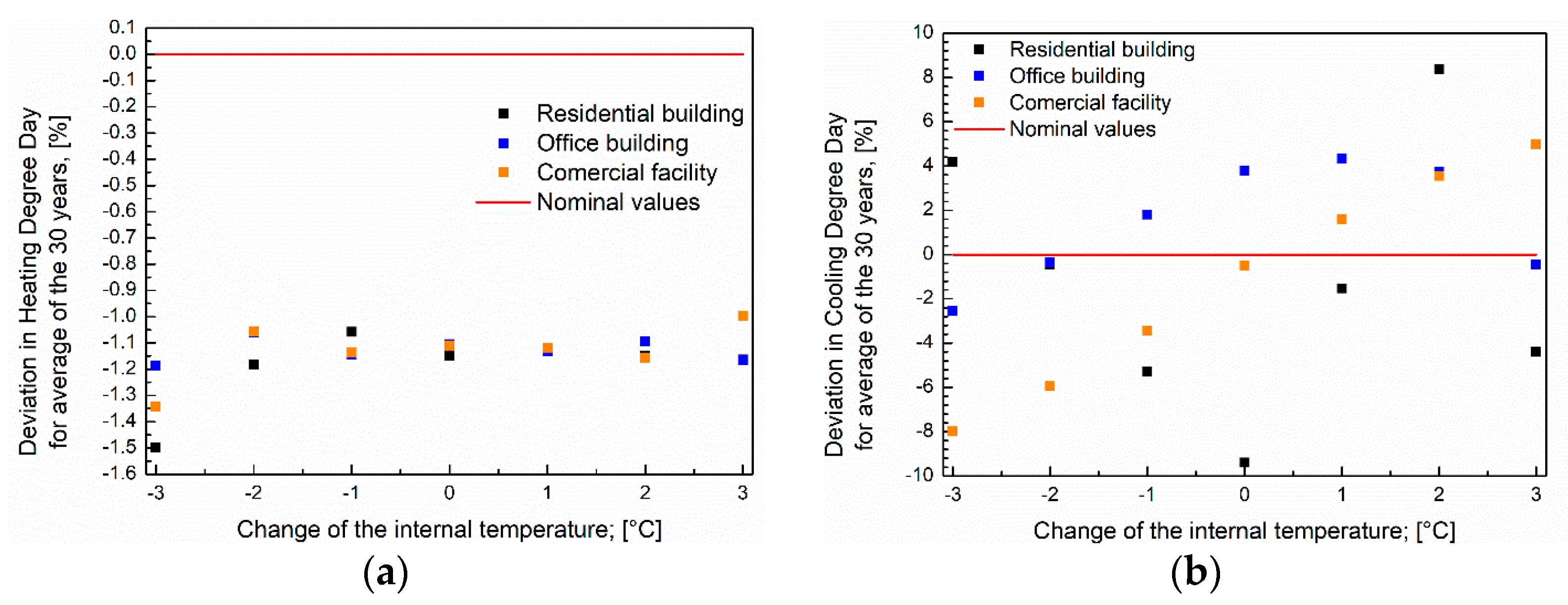
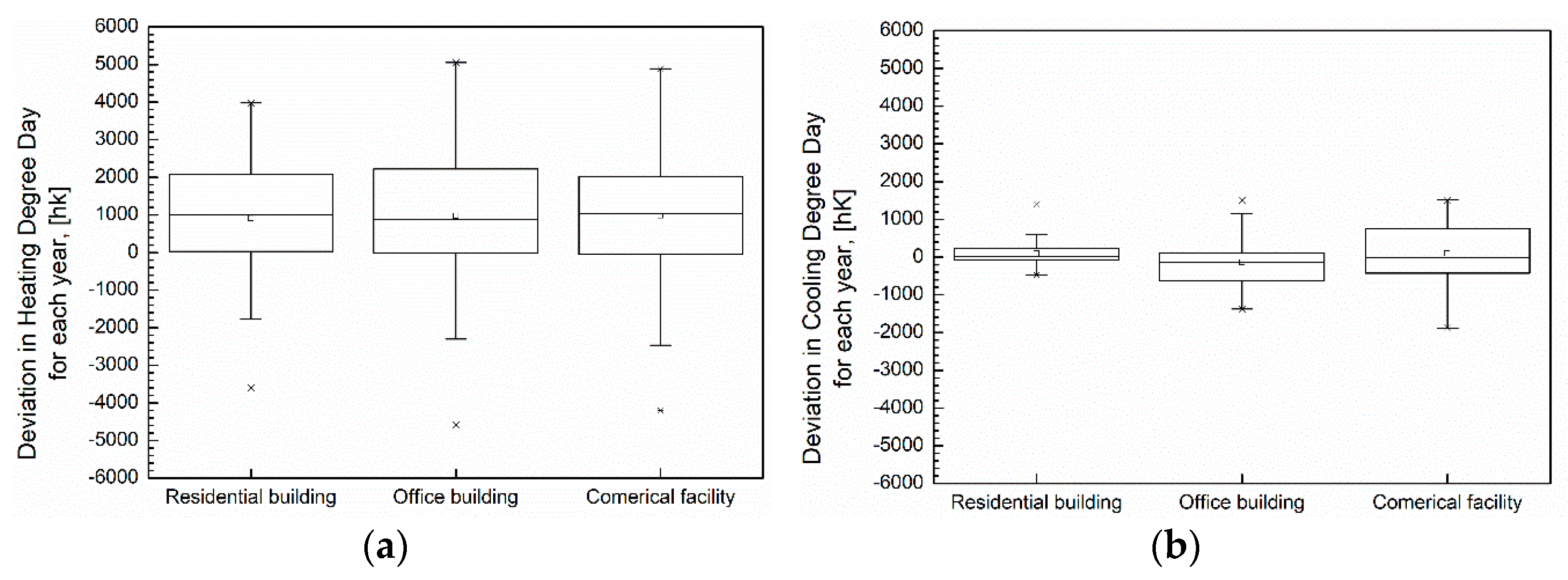
5.1. The Heating and Cooling Degree Day in Other Cities Using Equations

Temperature data for the cities of Szeged, Budapest, and Pécs, alongside Debrecen, were also measured by the Hungarian Meteorological Service (OMSZ). Furthermore, in the research conducted by Verbai et al. [38], the heating degree-day values in several Hungarian cities were also included. Therefore, a comparison can be made between the heating degree-day values determined from the measurements of OMSZ and these values. Similar heating degree-day values were obtained for Debrecen (76,490 [hK] and 75,600 [hK]) and Szeged (71,742 [hK] and 72,527 [hK]) at the same heating balance-point temperatures. However, there was a more significant difference for Budapest (72,390 [hK] and 66,592 [hK]) and Pécs (77,856 [hK] and 71,406 [hK]), respectively. This difference may be due to the difference between the years studied (1981–2010 and 1991–2020, respectively).

After this, the generalizability of Equations (6) and (7) was used by analyzing degree-day values for other cities in Hungary. The temperature values (measured by OMSZ) between 1991 and 2020 were considered for these respective locations.

Table 4. The deviation in the values of degree day (∆ti = 0), in %.

Title 1	Title 2	Debrecen	Szeged	Budapest	Pécs
Residential building	Heating	(−1.15)	(−1.19)	(−2.52)	(−1.82)
	Cooling	(−9.39)	6.48	20.67	(−4.77)
Office building	Heating	(−1.10)	(−1.34)	(−2.42)	(−1.83)
	Cooling	3.78	0.97	7.49	3.13
Commercial facility	Heating	(−1.11)	(−1.27)	(−2.36)	(−1.75)
	Cooling	(−0.50)	(−1.39)	(−2.19)	(−2.01)
Distance from Debrecen, [km]		0	181	195	305
Population, [people]		199,725	157,372	1,706,851	138,420

shows the deviations between the degree-day values calculated using Equations (6) and (7) and those determined with the daily mean temperature.

Based on the data presented in Table 4, similar values were observed in the heating case. However, a higher deviation was noticed in Budapest, which could be attributed to its larger population or the influence of the urban heat island effect.

In the cooling case, higher deviations were observed, and multiple factors could contribute to this phenomenon. Apart from differences in population size and the urban heat island effect, the distance from Debrecen also plays a significant role. The latter is due to the constants based on the Debrecen values from 1991 to 2020 in Equation (7).

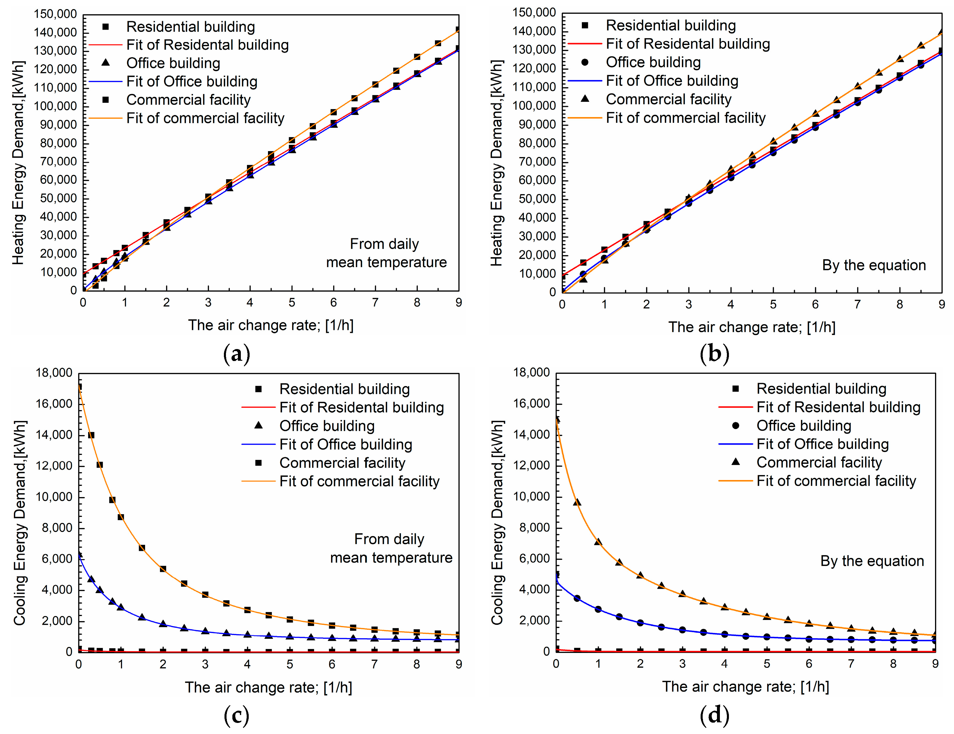
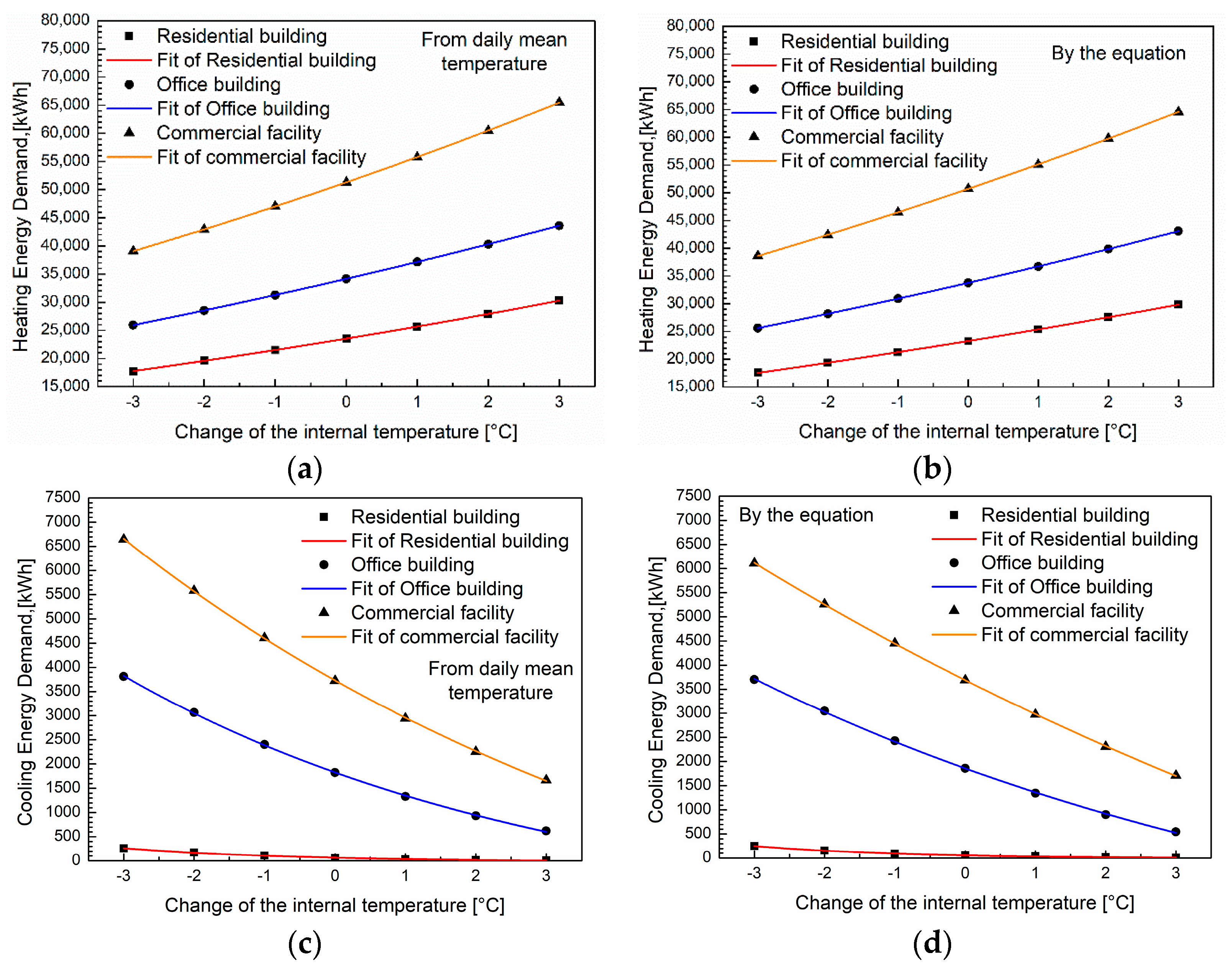
5.2. The Accuracy of the Determined Energy Demand Using the Equations

Figure 13 shows the deviation in energy demand compared with the energy demand determined using the daily mean temperature when utilizing the degree day calculated from the daily minimum and maximum temperatures. These deviations are presented as a function of the change in the air change rate.

The figures demonstrate a wave motion in the deviations. The higher the air change rate deviation, and the greater the air change rate, the smaller the deviation in energy demands will be. In other words, the relationships more and more accurately track the energy demand results determined from the daily mean temperature as the air change rate in the building increases.

Figure 14 depicts the variations in deviation from the energy demand determined using the daily mean temperature when calculated from the daily minimum and maximum temperatures. These variations are presented as a function of changes in the internal temperature.

Similar observations cannot be achieved while changing the internal temperature as when changing the air change rate. This is because the variation in the internal temperature is only ±10–16%, whereas the air change rate can range from −100% to +800%. But while it is realistic for the air change rate to decrease to close to zero (no mechanical ventilation, window with increased closure) or to rise to 9 1/h (mechanical ventilation), a change in the internal temperature of more than ±3 °C can cause significant comfort problems [39].

6. Conclusions

Striving for a more accurate determination of expected energy demand in buildings is becoming increasingly important in light of future energy crises. Novelty ideas are presented in this article that can contribute to this goal, followed by their application through a case study. The first idea is to consider a building’s function in determining energy demand. The second idea is to define HDD and CDD values based on daily minimum and maximum temperatures. The use of these two ideas through variations in internal temperature (±3 °C) and air change rate (ranging from 0 to 9 1/h) is examined in the case study.

Determining the function of a building plays a decisive role in terms of the number of people in the building and the amount of fresh air they require, daily human occupancy time, and controllability of the HVAC systems. Some of these factors influencing energy demand can be accounted for by a new efficiency (“η_U”), which is introduced in this article, while others indirectly manifest in the balance-point temperature. Therefore, it is highly relevant to consider the calculated values for each building rather than relying on a geographically determined base-point temperature. The case study findings demonstrate that a building with different functions can exhibit substantial disparities in heating energy demand. For example, a residential building requires only half as much as a commercial facility. Furthermore, cooling energy demands can present even higher differences.

Given the results from the case study, it can be concluded that the deviation in the HDD and CDD values calculated from the daily mean temperature compared with the values determined from the daily minimum and maximum temperatures is higher during the cooling season than during the heating season. However, the absolute differences in the heating season are significantly more, measured in [hK]. This fact is because, in Hungary, the value of HDD is generally higher than that of CDD. It should be mentioned that various inaccuracies were discovered during the HDD and CDD value calculations. These inaccuracies arose, for example, due to temperature measurements being taken only at four specific time points per day, which could be improved by collecting data at multiple time points throughout the day. In addition, the determination of daily minimum and maximum temperature values relied solely on the measurements taken at these four designated time points rather than considering the absolute minimum and maximum temperatures. Although the differences are expected to be negligible, using more accurate initial data would yield more precise results. Nevertheless, the developed equations are suitable for determining the HDD and CDD values, and, thus, the heating and cooling energy demand, when only two (daily minimum and maximum) temperatures are known.

References

1. Abergel, T.; Delmastro, C. Is cooling the future of heating? In International Energy Agency; IEA: Paris, France, 2020. [Google Scholar]
2. Hungarian Ministry of National Development. National Energy Strategy 2030; Hungarian Ministry of National Development: Budapest, Hungary, 2012. [Google Scholar]
3. Csáky, I. Analysis of Daily Energy Demand for Cooling in building with Different Comfort Categories—Case Study. Energies 2021, 14, 4694. [Google Scholar] [CrossRef]
4. Kalmár, F.; Kalmár, T. Thermal comfort aspects of solar gains during the heating season. Energies 2020, 13, 1702. [Google Scholar] [CrossRef] [Green Version]
5. Kutty, N.; Barakat, D.; Khoukhi, M. A French Residential Retrofit toward Achieving Net-Zero Energy Target in a Mediterranean Climate. Buildings 2023, 13, 833. [Google Scholar] [CrossRef]
6. Khourchid, A.M.; Al-Ansari, T.A.; Al-Ghamdi, S.G. Cooling Energy and Climate Change Nexus in Arid Climate and the Role of Energy Transition. Buildings 2023, 13, 836. [Google Scholar] [CrossRef]
7. Hamburg, A.; Mikola, A.; Parts, T.-M.; Kalamees, T. Heat Loss Due to Domestic Hot Water Pipes. Energies 2021, 14, 6446. [Google Scholar] [CrossRef]
8. Corcione, M.; Cretara, L.; Fontana, L.; Quintino, A. New Dimensionless Correlations for the Evaulation of the Thermal Resistances of a District Heating Twin Pipe System. Appl. Sci. 2021, 11, 9685. [Google Scholar] [CrossRef]
9. Kostyák, A.; Béres, C.; Szekeres, S.; Csáky, I. BufferTank Discharge Strategies in the Case of a Centrifugal Water Chiller. Energies 2023, 16, 188. [Google Scholar] [CrossRef]
10. Broin, E.Ó.; Nässén, J.; Johnsson, F. Energy efficiency policies for space heating in EU countries: A panel data analysis for the period 1990–2010. Appl. Energy 2015, 150, 211–223. [Google Scholar] [CrossRef] [Green Version]
11. Park, S.; Shim, J.; Song, D. Issues in calculation of balance-point temperatures for heating degree-days for the development of building-energy policy. Renew. Sustain. Energy Rev. 2021, 135, 110211. [Google Scholar] [CrossRef]
12. Szodrai, F. Analysis of a wall structure thermal transmittance sensitivity in function of meteorological parameters at constant internal surface temperature. In Proceedings of the AIP Conference Proceedings, Eger, Hungary, 29 September 2020. [Google Scholar] [CrossRef]
13. Cao, X.; Dai, X.; Liu, J. Building energy-consumption status worldwide and the state-of-the-art technologies for zero-energy building during the past decade. Energy Build. 2016, 128, 198–213. [Google Scholar] [CrossRef]
14. Pérez-Andreu, V.; Aparicio-Fernández, C.; Martínez-Ibernón, A.; Vivancos, J.-L. Impact of climate change on heating and cooling energy demand in a residential building in a Mediterranean climate. Energy 2018, 165, 63–74. [Google Scholar] [CrossRef]
15. Ciancio, V.; Salata, F.; Falasca, S.; Curci, G. Energy demands of buildings in the framework of climate change: An investigation across Europe. Sustain. Cities Soc. 2020, 60, 102213. [Google Scholar] [CrossRef]
16. Morakinyo, T.E. Estimates of the impact of extreme heat event on cooling energy demand in Hong Kong. Renew. Energy 2019, 142, 73–84. [Google Scholar] [CrossRef]
17. Bodó, B.; Kalmár, F. Analysis of primary energy use of typical buildings in Hungary. Environ. Eng. Manag. J. 2014, 13, 2725–2731. [Google Scholar] [CrossRef]
18. Krese, G.; Lampret, Ž.; Butala, V.; Prek, M. Determination of a Building’s balance point temperature as an energy characteristic. Energy 2018, 165, 1034–1049. [Google Scholar] [CrossRef]
19. Sivak, M. Potential energy demand for cooling in the 50 largest metropolitan areas of the world: Implications for developing countries. Energy Policy 2009, 37, 1382–1384. [Google Scholar] [CrossRef]
20. Olonscheck, M.; Holsten, A.; Kropp, J.P. Heating and cooling energy demand and related emissions of the German residential building stock under climate change. Energy Policy 2011, 39, 4795–4806. [Google Scholar] [CrossRef]
21. Mohareb, E.A.; Kennedy, C.A.; Harvey, L.D.D.; Pressnail, K. Decoupling of Building Energy Use and Climate. Energy Build. 2011, 43, 2961–2963. [Google Scholar] [CrossRef]
22. Harvey, L.D.D. Using modified multiple heating-degree-day (HDD) and cooling-degree-day (CDD) indices to estimate building heating and cooling loads. Energy Build. 2020, 229, 110475. [Google Scholar] [CrossRef]
23. Harvey, L.D.D. A Handbook on Low-Energy Buildings and District-Energy Systems, 1st ed.; Taylor & Francis: London, UK, 2006; pp. 21–36. [Google Scholar]
24. The European Parliament and of the Council, Directive 2010/31/EU of the European Parliament and of the Council. Off. J. Eur. Union 2010, 153, 13–35.
25. Bardhan, R.; Debnath, R.; Gama, J.; Vijay, U. REST framework: A modelling approach towards cooling energy stress mitigation plans for future cities in warming Global South. Sustain. Cities Soc. 2020, 61, 102315. [Google Scholar] [CrossRef] [PubMed]
26. Verbai, Z.; Csáky, I.; Kalmár, F. Balance point temperature for heating as a function of glazing orientation and room time constant. Energy Build. 2017, 135, 1–9. [Google Scholar] [CrossRef]
27. Hekkenberg, M.; Moll, H.C.; Uiterkamp, A.J.M. Dynamic temperature dependence patterns in future energy demand models in the context of climate change. Energy 2009, 34, 1797–1806. [Google Scholar] [CrossRef]
28. Lee, K.; Baek, H.-J.; Cho, S. The Estimation of Base Temperature for Heating and Cooling Degree-Days for South Korea. J. Appl. Meteorol. Climatol. 2014, 53, 300–309. [Google Scholar] [CrossRef]
29. Mourshed, M. Relationship between annual mean temperature and degree-days. Energy Build. 2012, 54, 418–425. [Google Scholar] [CrossRef] [Green Version]
30. Azevedo, J.A.; Chapman, L.; Muller, C. Critique and suggested modifications of the degree day methodology to enable long term electricity consumption assessments; a case study in Birmingham, UK. Meteorol. Appl. 2015, 22, 789–796. [Google Scholar] [CrossRef]
31. Karlsson, J.; Roos, A.; Karlsson, B. Building and climate influence on the balance temperature of buildings. Build. Environ. 2003, 38, 75–81. [Google Scholar] [CrossRef]
32. Meng, Q.; Xi, Y.; Zhang, X.; Mourshed, M.; Hui, Y. Evaluating multiple parameters dependency of base temperature for heating degree-days in building energy prediction. Build. Simul. 2021, 14, 969–985. [Google Scholar] [CrossRef]
33. Kheiri, F.; Haberl, J.S.; Baltazar, J.-C. Split-degree day method: A novel degree day method for improving building energy performance estimation. Energy Build. 2023, 134, 154–161. [Google Scholar] [CrossRef]
34. Day, T. Degree Days: Theory and Application; Chartered Institution of Building Services Engineers: London, UK, 2006. [Google Scholar]
35. ASHRAE 55. Ashrae Handbook Fundamentals; ASHRAE: Peachtree Corners, GA, USA, 2017. [Google Scholar]
36. Larsen, M.A.D.; Petrović, S.; Radoszynski, A.M.; McKenna, R.; Balyk, O. Climate change impacts on trends and extremes in future heating and cooling demands over Europe. Energy Build. 2020, 226, 110397. [Google Scholar] [CrossRef]
37. Salata, F.; Falasca, S.; Ciancio, V.; Curci, G.; Grignaffini, S.; Wilde, P. Estimating building cooling energy demand through the Cooling Degree Hours in a changing climate: A modeling study. Sustain. Cities Soc. 2021, 76, 103518. [Google Scholar] [CrossRef]
38. Verbai, Z.; Lázár, I.; Kalmár, F. Heating degree day in Hungary. Environ. Eng. Manag. J. 2014, 13, 2887–2892. [Google Scholar] [CrossRef]
39. Szabó, G.L.; Kalmár, F. Investigation of subjective and objective thermal comfort in the case of ceiling and wall cooling systems. Int. Rev. Appl. Sci. Eng. 2017, 8, 153–162. [Google Scholar] [CrossRef] [Green Version]
Figure 1. (a) Degree-day curves, (b) understanding the degree days.
Buildings 13 01905 g001
Figure 2. Changes in daily temperatures.
Buildings 13 01905 g002
Figure 3. Determination of the utilization efficiency for a building.
Buildings 13 01905 g003
Figure 4. The interior layout of the building for (a) residential building; (b) office building; (c) commercial facility.
Buildings 13 01905 g004
Figure 5. The effect of air change rate on the balance-point temperature during (a) heating and (b) cooling seasons.
Buildings 13 01905 g005
Figure 6. The varying degree day as a function of air change rate during the (a) heating, (b) cooling season.
Buildings 13 01905 g006
Figure 7. The varying degree day as a function of internal temperature change during the (a) heating, (b) cooling season.
Buildings 13 01905 g007
Figure 8. The calculated degree-day values (Δti = 0) during the (a) heating and (b) cooling season.
Buildings 13 01905 g008
Figure 9. The deviation from the degree-day values determined from the daily mean temperature for each building function, using the equations for the (a) heating and (b) cooling season.
Buildings 13 01905 g009
Figure 10. The deviation in degree days to the nominal values for each year during the (a) heating, (b) cooling season.
Buildings 13 01905 g010
Figure 11. The energy demand of the building depending on the air change rate (a) during the heating season, based on daily mean temperature; (b) during the heating season, based on daily minimum and maximum temperature; (c) during the cooling season, based on daily minimum and maximum temperature; (d) during the cooling season, based on daily minimum and maximum temperature.
Buildings 13 01905 g011
Figure 12. The energy demand of the building depending on changing the internal temperature (a) during the heating season, based on daily mean temperature; (b) during the heating season, based on daily minimum and maximum temperature; (c) during the cooling season, based on daily mean temperature; (d) during the cooling season, based on daily minimum and maximum temperature.
Buildings 13 01905 g012
Figure 13. The deviation in the heating and cooling energy demand by using equations (∆ti = 0 °C) for (a) residential building; (b) office building; (c) commercial facility.
Buildings 13 01905 g013
Figure 14. The deviation in the (a) heating and (b) cooling energy demand by using equations (n = nnom).
Buildings 13 01905 g014