Article

A Hybrid Deep Learning Approach for Real-Time Estimation of Passenger Traffic Flow in Urban Railway Systems

1
School of Civil and Environmental Engineering, Nanyang Technological University, 50 Nanyang Avenue, Singapore 639798, Singapore
2
Hubei Jianke Technology Group, Wuhan 430223, China
3
School of Civil and Hydraulic Engineering, Huazhong University of Science and Technology, 1037 Luoyu Road, Hongshan District, Wuhan 430074, China
*
Author to whom correspondence should be addressed.
Buildings 2023, 13(6), 1514; https://doi.org/10.3390/buildings13061514
Submission received: 25 August 2022 / Revised: 3 November 2022 / Accepted: 25 November 2022 / Published: 12 June 2023

Abstract

:
This research introduces a hybrid deep learning approach to perform real-time forecasting of passenger traffic flow for the metro railway system (MRS). By integrating long short-term memory (LSTM) and the graph convolutional network (GCN), a hybrid deep learning neural network named the graph convolutional memory network (GCMN) was constructed and trained for accurate real-time prediction of passenger traffic flow for the MRS. Data collected of the traffic flow in Delhi’s metro rail network system in the period from October 2012 to May 2017 were utilized to demonstrate the effectiveness of the developed model. The results indicate that (1) the developed method provides accurate predictions of the traffic flow with an average coefficient of determination (R2) of 0.920, RMSE of 368.364, and MAE of 549.527, and (2) the GCMN model outperforms state-of-the-art methods, including LSTM and the light gradient boosting machine (LightGBM). This study contributes to the state of practice in proposing a novel framework that provides reliable estimations of passenger traffic flow. The developed model can also be used as a benchmark for planning and upgrading works of the MRS by metro owners and architects.

1. Introduction

The railway industry has formed one of the most bustling networks in the world. Within densely populated and physically vast cities, metros are gradually becoming an integral feature of modern transportation networks. They relieve traffic congestion on roadways while also providing a more ecologically friendly alternative to driving personal automobiles. A growing number of cities are evolving in this manner, which consequently necessitates that trains operate with better efficiency and higher capacity [1]. To meet these increasing demands, in this work, information technologies (IT) are investigated to assist the railway industry to achieve better performance in terms of robustness, reliability, and capacity [2]. Therefore, the successful operation of metro railway systems (MRS) is dependent on the meticulousness of their metro service planning in order to ensure that the system operates in accordance with commuter demands and necessities [3].
Forecasting passenger traffic flow is an important aspect of effective transportation management. However, passenger traffic flow is very unpredictable and is influenced by a variety of internal and external variables. As a result, predicting passenger flow is a complicated process that necessitates the use of effective adaptive systems [4,5]. Temporal intrinsic influencing characteristics are possible where the placement of the stations and passenger movement at the nearby stations are the primary spatial impacts. Intra-sequential statistical relationships among successive flow data are the main sources of temporal impacts. The system’s final performance is determined by the right mix of both features. Using a recurrent neural network, this research presents a unique technique to combine the two impacts to form an intermediate feature space [6].
Researchers have applied various approaches to forecasting traffic in metropolitan areas in order to encourage the practice of the urban transportation services of aiding metropolises in providing comfortable railway and bus services [7]. According to the literature, statistical methods and the intelligent method are the two major types of approaches that been widely applied. The statistical methods normally apply developed statistical models to fit the data. For instance, Nihan et al. [8] employed the Box and Jenkins time series to anticipate short-term traffic flow on expressways in 1980. Sun et al. [9] utilized a linear regression model to estimate traffic volume. With advancements in artificial intelligence technologies, the focus was shifted to machine learning approaches, which gave researchers a path to focus their efforts on intelligent transportation systems [10]. For example, Castillo et al. [11] adopted a Bayesian network technique to anticipate traffic volume. Hong et al. [12] employed support vector regression (SVR) method to predict traffic flow. Although these studies have demonstrated the applicability of the proposed methods, there are limitations that warrant further investigation. The MRS’s passenger traffic flow forecast may be viewed as a time series prediction problem where both historical data of the traffic flow and other factors will affect the traffic flow. However, the methods applied in previous studies considered either the temporal factor of time series data or the spatial factor of the other influential factors, and there is a lack of consideration of both factors. Therefore, this study intends to investigate a method that considers both factors for a prediction of traffic flow with better accuracy.
The deep learning approach has had great success with time series predictions including speech recognition and picture recognition, among other things. Among the different types of deep learning neural networks been established, long short-term memory (LSTM) and graph convolutional networks (GCNs) are two types of networks that have a wide application with positive results in many studies. LSTM has good capabilities in processing time series data, while GCNs focus on extracting the spatial features from graph data. The combination of GCNs and LSTM has also been investigated with successful application in road traffic [13] and tunneling works [14]. However, it has not been investigated in relation to metro traffic flow prediction. Therefore, this study aimed to extract spatial and temporal features using time series data and to predict the MRS passenger traffic flow by developing a hybrid model. To perform these tasks, a novel deep learning network named the graph convolutional memory network (GCMN) was constructed by integrating GCN and LSTM networks. The developed model enables metro owners and architects to better evaluate and manage MRS planning and upgrading works, eventually leading to improved user satisfaction and technology acceptance for the MRS.
The focus of this research will be whether (1) a hybrid model combining LSTM and GCN neural networks would increase the accuracy of predicting MRS passenger traffic volume, and (2) in terms of the accuracy and efficiency of the algorithm, different historical timesteps in the sequence data supplied into the prediction model will alter the forecast outcomes of the MRS’s passenger traffic flow. To address these challenges, this study developed a GCMN-based model for MRS passenger traffic flow time series prediction that contributes to (a) the development of a hybrid model by combining LSTM and GCNs into a time series prediction model to improve forecasted accuracy for the MRS’s passenger traffic volume, which may provide new perspectives for other predictive problems in general, and (b) the production of a prediction-based control method for reliable real-time estimation of the MRS’s passenger traffic volume.
The rest of the paper is organized as follows. A literature review on passenger traffic flow is presented in Section 2. The prediction methodologies and procedures employed in this work are explained in Section 3. Section 4 discusses a case study of the concept involving the Delhi Metro, which is part of India’s metro rail network system project. Section 5 analyzes the evaluation of the performance of the model through a comparison with two other models. Lastly, Section 6 presents the conclusion of this study with future work suggestions and recommendations.

2. Literature Review

Currently, many stations have installed sophisticated measurement systems and a variety of intelligent technologies, resulting in metro traffic volume data that are suitable for fitting computational models. To forecast passenger flow, a variety of different methods have been investigated which can generally be categorized as single models or hybrid models.
There are many scholars investigating traffic flow estimation by adopting the existing statistical and intelligence methods as a single model. The statistical approaches generally predict traffic flow by fitting the data with well-developed models, such as the autoregressive integrated moving average (ARIMA) approach, and the B-spline method [15,16,17]. The intelligence methods mainly use machine learning approaches to map the relationship between passenger flow and other traffic factors, and include artificial neural networks [18], deep belief networks [19], and LSTM neural networks [20], which were adopted to predict traffic flow, average vehicle moving speed, mean traffic time, etc.
To improve accuracy, researchers have looked into ways to hybridize the existing methods for passenger flow and traffic forecasts, such as a Kalman filter neural network used to estimate traffic flow for a medium-sized network by Chen et al. [21]; neural networks and ARIMA models for transit ridership predicted using regression analysis by Chiang et al. [22]; moving average aggregation, exponential smoothing, ARIMA, and neural network models for traffic flow prediction by Tan et al. [23], two neural network topologies designed and combined for railway passenger demand forecasting by Tsai et al. [24], etc. Although many studies have proven the applicability of the proposed method with positive results, there is a lack of consideration for both temporal and spatial factors to improve the prediction with higher accuracy.
The deep neural network has been investigated by many scholars with positive results in many domains of science. Among the numerous models proposed, Zhao et al. [13] proposed a deep neural network that integrates the GCN and LSTM structures and obtained positive results for traffic flow estimation on the road. A similar approach was also investigated by Fu et al. [14] for the estimation of the trajectory deviations of tunnel boring machines (TBM). Motivated by the effectiveness of this method, this study intends to hybridize the GCN and LSTM cells and propose a model that can incorporate both spatial and temporal factors for an accurate estimation of rail network traffic flow.

3. Methodology

LSTM and GCN are used as time series predictions in this developed model to properly estimate the traffic volume flow in metros of megalopolises. This section explains the suggested approach, as outlined in Figure 1 below.

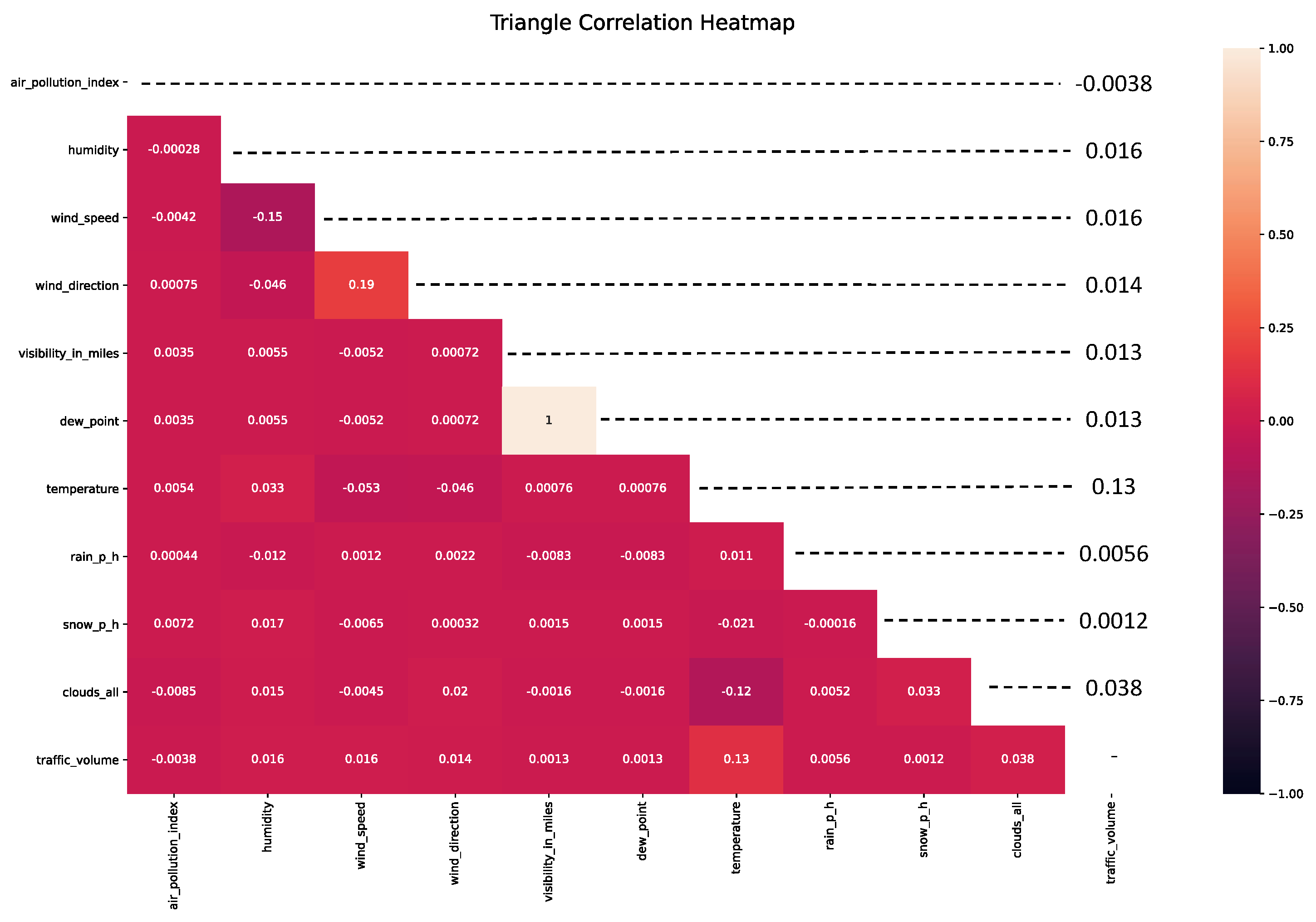
3.1. Data Collection, Processing, and Feature Selection

This study exhibits the data from Delhi’s metro rail network system presented as a comma-separated value (CSV) file according to date and time. These files contain all of the monitoring data collected during rail transit in metro systems. Furthermore, these data consist of a range of information regarding the transit process, including the operation date and time, pollution index, wind speed and direction, visibility, temperature, etc. However, the records contain erroneous, redundant, and noisy data due to processing errors such as invalid or zero-valued cells, repetitive data, extreme values and other noises. As a result, data preparation is required to clean, sort, and convert the data before it can be fitted into the model that will be used to train the proposed GCMN neural network.
Data cleaning, rescaling, and reframing are techniques of data preparation. Data cleaning is required to eliminate erroneous data such as zero-valued and null cells from the data since these may provide superfluous information to the neural network. The information delivered to the proposed model is more clear, concise, and accurate with the data cleansed. Next, due to the data extracted for rail transit analysis having varying magnitudes, data rescaling is necessary to lower the neural network’s computational time which influences the model’s performance. Before being implemented in the model, all features were rescaled in the range of 0 to 1 in this study. Lastly, the input variables are normalized and the dataset is reframed as a time series supervised learning problem. Predicting the input parameters at the next timestep,  t , given the input parameters at the previous timestep,  t 1 , is established as a supervised learning problem. Let  x n = { x 1 ,   x 2 ,   x 3 , , x n }  be the input parameter data, where  x 1 ,   x 2 ,   x 3 , , x n  corresponds to the data extracted for rail transit analysis chosen for this forecasting technique, and f( x i ) be the determining function for these parameters with  F  as the multiplication result for all determining functions. Additionally, let the current timestep of the input parameter data be  t  where the prior timestep will, respectively be  t 1 . If any single attribute in the input data,  x i  is zero-valued or invalid, it will result in f ( x i ) = 0 and in  F = 0 . On that account, this row of input data will be recognized as invalid and removed accordingly. Data cleaning, rescaling, and reframing techniques are illustrated in Equations (1)–(4) below:
F = f ( x 1 ) f ( x 2 ) f ( x 3 ) f ( x n )
f ( x 1 ) = { 1         x j 0 0           x j = 0  
x j = x i x m i n x m a x   x m i n
x = [ x 1 ,   t n x 1 ,   t n + 1 x 1 ,   t 1 x 1 ,   t x 2 ,   t n x 2 ,   t n + 1 x 2 ,   t 1 x 2 ,   t x k 1 ,   t n x k 1 ,   t n + 1 x k 1 ,   t 1 x k 1 ,   t x k ,   t n x k ,   t n + 1 x k ,   t 1 x k ,   t ]
When constructing a predictive model, to further evaluate the link between each input variable and the goal output variable, the calculation of the correlation score between input variables using statistical measures aids in comprehending the relationship between the input variables and goal variable. Pearson correlation was chosen to further analyze and filter the variables available by computing the best scores against the output to generate the inputs for the predictive model in this paper’s feature selection. Pearson’s correlation coefficient is a measure of the strength commonly denoted in statistical models as the r value between any two variables where the best fit line is drawn through the data of the two variables and returns as the correlation strength value by computing the covariance of two variables and then dividing it by the product of their standard deviations. Moreover, this also denotes that the distance between the best fit line and the data points of the coefficient is not affected by different scales of the input and output variables as illustrated in Equation (5) below [25,26]
r = ( x i x ¯ ) ( y i y ¯ ) ( x i x ¯ ) 2 ( y i y ¯ ) 2
where  r  is the Pearson correlation coefficient,  x i  is the  x  input variable samples,  x ¯  is the mean of values in  x  variable,  y i  is the  y  output variable samples and  y ¯  is the mean of values in  y  variable.

3.2. PCMCI Enabled Causal Discovery

For this study, in addition to a feature matrix from the dataset, the GCN model also necessitates an adjacency matrix to create a filter in the Fourier domain and generate real-time prediction. Therefore, a casual network discovery method, which is an effective tool for discovering the true relationships in complex systems, is selected to generate an adjacency matrix for the model as a second input dataset for the GCN neural network component of the T-GCN model. PCMCI is a large-scale time series task-specific causal discovery framework. Additionally, PCMCI identifies causal structure using a time-delayed graphical model in which causal relationships are approximated and time lags in a complex system are provided. Conceptual diagram of the causal network discovery are shown in Figure 2.
The PCMCI algorithm is performed in two phases:  PC 1  condition selection and momentary conditional independence (MCI) test. For all included time series variables  j { 1 , , N } PC 1  condition selection is used to find important conditions  P ^ ( X t j )  and eliminate irrelevant conditions, while the MCI test limits false-positive rate by testing if  X t τ i X t j  with Equation (6) [27,28].
MCI :   X t τ i X t j   |   P ^ ( X t j ) ,   P ^ ( X t τ i )
where MCI conditions on both parents are  X t j  and  X t τ j PC 1  is a Markov set discovery algorithm based on the PC algorithm that uses iterative independence testing to eliminate unnecessary circumstances for each N variable. Following that, the MCI test was used to handle the false-positive control of time series data [27,28], and the causal links between the variables were established accordingly.

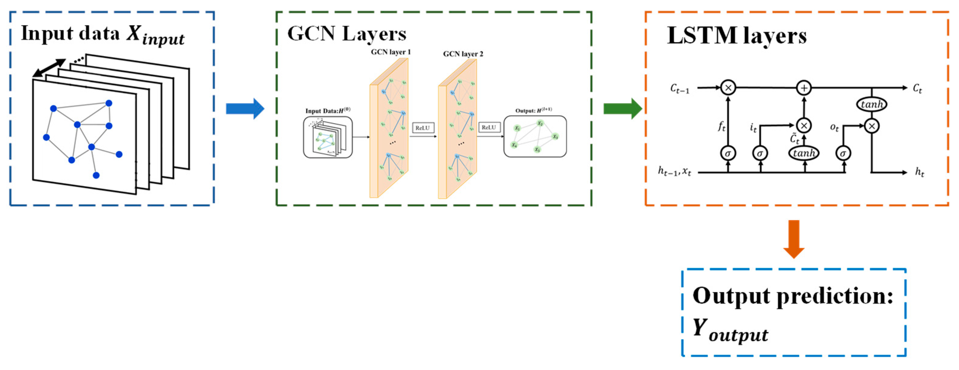
3.3. Model Development GCMN

The GCMN model consists of two neural network parts: the GCN neural network and the LSTM neural network. The proposed GCMN model can be trained for real-time traffic volume prediction after data preparation for data cleansing, data rescaling, and data reframing has been completed. This section outlines three aspects of the real-time prediction of the GCMN model: (1) LSTM model, (2) GCN model, and (3) model training and prediction.

3.3.1. Structure of LSTM Cells

The LSTM’s design serves as a memory cell that preserves some information over time. This is achieved by by introducing three additional gate structures named as input gate, forget gate, and output gate. These gates within the conventional LSTM cell help to mitigate the potential gradient disappearance and gradient explosion during model training, effectively compensating for the drawbacks of a simple RNN model. Considering the current time as  t , the information delivered from the previous cell state,  t 1 , is denoted as  h t 1 . For this study, three parameters are included in the LSTM neural network’s output: sample, timestep, and feature dimension. The amount of previous datasets employed to anticipate the data for the future time is determined by the timestep value. Such function enables the LSTM neural network to extract features from time series data in order to increase prediction accuracy.
Refer to the typical LSTM cell structure in Figure 3; the typical process of the LSTM comprises the input information from the current time,  x n , t , passing through the forget gate,  f t . This gate will determine which information are to be retained from the cell state of previous time step, which is achieved through the sigmoid activation function,  σ , where  σ = 1 1 + e x . Next, the input gate decides on selected information to preserve in the current cell state,  C t  where the activation function,  tanh = e x e x e x + e x  is used to generate a new memory  C t ˜  that is added to the cell state. Then, the output gate,  o t  resolves information for the next timestep. The above-mentioned calculating technique for the LSTM memory cell is as follows, where  C t  and  h t  are further calculated according to Equations (12) and (13):
f t = σ ( w f [ x n , t , h t 1 ] + b f )
i t = σ ( w i [ x n , t , h t 1 ] + b i )
o t = σ ( w o [ x n , t , h t 1 ] + b o )
C t ˜ = σ ( w c [ x n , t , h t 1 ] + b c )
C t = f t C t 1 + i t C t ˜
h t = o t tan h ( C t )
where  w f w i w o , and  w c  represent the weight coefficient matrix for the forgetting gate, the input gate, the output gate, and the neuron state matrix, respectively, and  b f b i b o  and  b c  are the bias for the corresponding gates, respectively.

3.3.2. Structure of GCN Cells

To obtain spatial dependency, the GCN model’s structure learns spatial aspects from TBM’s data. The GCMN model would be able to acquire and encode the topological correlations between the deviation and its input variables assuming node 1 depicts the traffic volume flow of passengers. Using an adjacency matrix,  A , and a feature matrix,  X , the GCN model creates a filter that transforms the nodes of a graph to capture the spatial characteristics between the nodes that are computed by the GCN model’s layered multiple convolutional layers. Equations (13) and (14) below describe the transformation of the GCN model’s computation of layered multiple convolutional layers and the two-layer GCMN model used in this research:
H ( l + 1 ) = σ ( D ˜ 1 2 A ^ D ˜ 1 2 H ( l ) θ ( l ) )
f ( X , A ) = σ ( A ^   ReLU   ( A ^ X W 0 )   W 1 )
where  H ( l )  denotes the  l t h  layer of the output,  σ ( · )  represents the sigmoid function,  D   ˜  computes the degree matrix,  D   ˜ = j A ˜ i j θ ( l ) , and  A ^ = D ˜ 1 2 A ˜ D ˜ 1 2  calculates the preprocessing step with  A ˜ = A + I N  whereby  A ˜  is the adjacency matrix and  I N  is the identity matrix. Additionally, the weight matrix from the input layer to the first hidden layer is denoted as  W 0 R P · H  and the weight matrix from the first hidden layer to the second hidden layer is represented as  W 1 R H · T . Thus,  f ( X , A ) R N · T  computes the output with prediction length  T , with the activation function as ReLU. The typical structure of GCN layers is shown in Figure 4.

3.3.3. GCMN Model Training and Prediction

The GCMN model is trained to estimate the traffic volume flow in real time following data preparation consisting of data purification, data rescaling, and data reframing. To train and validate the proposed method, the preprocessed data are separated into two groups, namely, the training group and the testing group, with  X t r a i n  and  Y t r a i n  denoting the input and output data for training and  X t e s t  and  Y t e s t  for testing. The model is trained by the input data,  X t r a i n , over 30 epochs to predict the output data,  Y t r a i n , where each epoch is assessed for its accuracy. Next, for model performance analysis, the test input data,  X t e s t  is predicted and compared to  Y t e s t .
TensorFlow Keras and StellarGraph frameworks are modules in Python used with two sets of data necessary for the training procedure, with the first input data being the correlation metrics generated by running the PCMCI algorithm on the time series data, and the second being the original dataset in the form of an  n × n  metric and  k ( n + 1 )  metric, which are known as  X c o r r  and  X i n p u t  correspondingly. All the variables,  x i , j  for time,  t  for  x 1  to  x k  at time sequence  t n  to  t  are considered as the inputs for real-time prediction. Then,  x k  at the time,  t  that is denoted as  x k , t  or  Y o u t p u t  which is the output for prediction. Additionally, for the two necessary input datasets, input  X  has their corresponding output  Y . These are described in Equations (15)–(18) below:
x i , j = f { x 1 , t n , x 2 , t n , , x k 1 , t 1 , x k , t 1 }
X i n p u t = [ x 1 ,   t n x 1 ,   t n + 1 x 1 ,   t 1 x 1 ,   t x 2 ,   t n x 2 ,   t n + 1 x 2 ,   t 1 x 2 ,   t x k 1 ,   t n x k 1 ,   t n + 1 x k 1 ,   t 1 x k 1 ,   t x k ,   t n x k ,   t n + 1 x k ,   t 1 x k ,   t 1 ]
X c o r r = [ 1 P ( x 1 ,   t n + 1 ) P ( x 1 ,   t 1 ) P ( x k 1 ,   t ) P ( x 2 ,   t n ) 1 P ( x 2 ,   t 1 ) P ( x 2 ,   t ) P ( x k 1 ,   t n ) P ( x k 1 ,   t n + 1 ) 1 P ( x k 1 ,   t ) P ( x k ,   t n ) P ( x k ,   t n + 1 ) P ( x k ,   t 1 ) 1 ]
Y o u t p u t = x k ,   t
where  i  represents the input parameters,  j  represents the time stamp with the current timestamp  x k ,   t  replaced with  x k ,   t 1 , the function  P  represents the execution of the PCMCI algorithm, and  P ( x 2 ,   t n )  represents the results generated from the PCMCI algorithm. The case study in Section 4 is used to discuss the model’s efficacy.

3.4. Model Evaluation

Deep learning models are assessed in order to determine their accuracy. The prediction outputs of the model are compared against the test dataset to verify the prediction accuracy from the proposed model. By comparing the prediction with the test dataset’s actual values, the results are assessed using standard statistical criteria including mean absolute error (MAE), root mean squared error (RMSE), and R-squared ( R 2 ). MAE represents the average magnitude of difference between the prediction and the ground truth in absolute manner, while RMSE focus more on the the standard deviation of the forecast error. Despite the fact that MAE and RMSE both measure the average prediction error, MAE provides an unbiased average of the error, whereas RMSE is biased when samples with bigger mistakes are weighted more heavily.  R 2  is a statistical measure of fitness that shows how much variance of the testing data is explained by the prediction models [29]. In this study,  R 2  is used to compare the accuracy of the test data with the predicted results, where an  R 2  of 1 indicates that the projected results have accurately predicted the test data. MAE, RMSE,  R 2  and MSE can be calculated by Equations (19)–(21) as below, respectively:
MAE = 1 n   i = 1 n | y i y ^ |
RMSE = i = 1 n ( y i y ^ ) 2 n
R 2 = 1 t = 1 n ( y i y ^ ) 2 t = 1 n ( y i y ¯ ) 2
where  n  is total amount of testing data,  y ( i )  is the  i t h  measurement,  y ^ ( i )  is its corresponding prediction,  y ¯  is the mean value of ground truth, and  f i ( x )  is the predicted value.
Additionally, a GCMN model consisting of two GCN layers and two LSTM layers is proposed, where each GCN layer and both LSTM layers incorporate 16, 10, and 256 nodes, respectively. The GCN layers’ activation function is a rectified linear unit ( ReLU ), whereas the LSTM layers’ activation function is an exponential linear unit ( ELU ). The optimizer for this model is Adam and the loss function is MSE. The activation functions are described in Equations (22) and (23) below.
RELU ( x ) = { x ,     if   x > 0 0 ,     if   x 0
ELU ( x ) = { x , if   x > 0 α ( exp ( x ) 1 ) , if   x 0
where  α = 1  in most of the cases. An illustration of the GCMN model is shown in Figure 5.

4. Case Study

This case study was conducted with traffic flow data collected from Delhi’s metro rail network to validate the effectiveness of the proposed GCMN approach, where the traffic flow data was extracted from Kaggle (see the link https://www.kaggle.com/datasets/umairnsr87/indian-metro-data). This chapter includes extensive explanations on the project outline, training, and prediction on the GCMN-based model, and analyses of the findings for each are described in Section 4.1, Section 4.2, and Section 4.3, respectively.

4.1. Case Background and Data Collection

The Delhi Metro is the largest MRS in India’s metro rail network system, spanning 347 km in an urban mass rapid transit system built with 10 lines and 253 stations. This research selected daily monitored data obtained from Delhi’s metro network for the years between October 2012 and May 2017 [30], where the extracted MRS traffic flow data were processed and stored in a CSV file. Since weather could be one of the major factors that affect passenger traffic flow in the rail system, a total of around 33,750 rows of raw data consisting of 10 attributes of weather factors were extracted as the inputs for the case study.
The extracted input parameters were air pollution index ( x 1 ), humidity ( x 2 ), wind speed ( x 3 ), wind direction ( x 4 ), visibility in miles ( x 5 ), dew point ( x 6 ), temperature ( x 7 ), rain per hour ( x 8 ), snow per hour ( x 9 ), and clouds all ( x 10 ), while the passenger traffic flow ( y ) was extracted as the output parameter. A description of the 11 input and output attributes and a data description are presented in Table 1 and Table 2, respectively. Additionally, the hour, date, and time variable is also removed, which leaves 11 features in addition to their statistical interpretations remaining. For a better understanding of the data, the correlation of the input attributes with the output as well as a triangle heatmap for the correlation between all variables are shown in Figure 6.

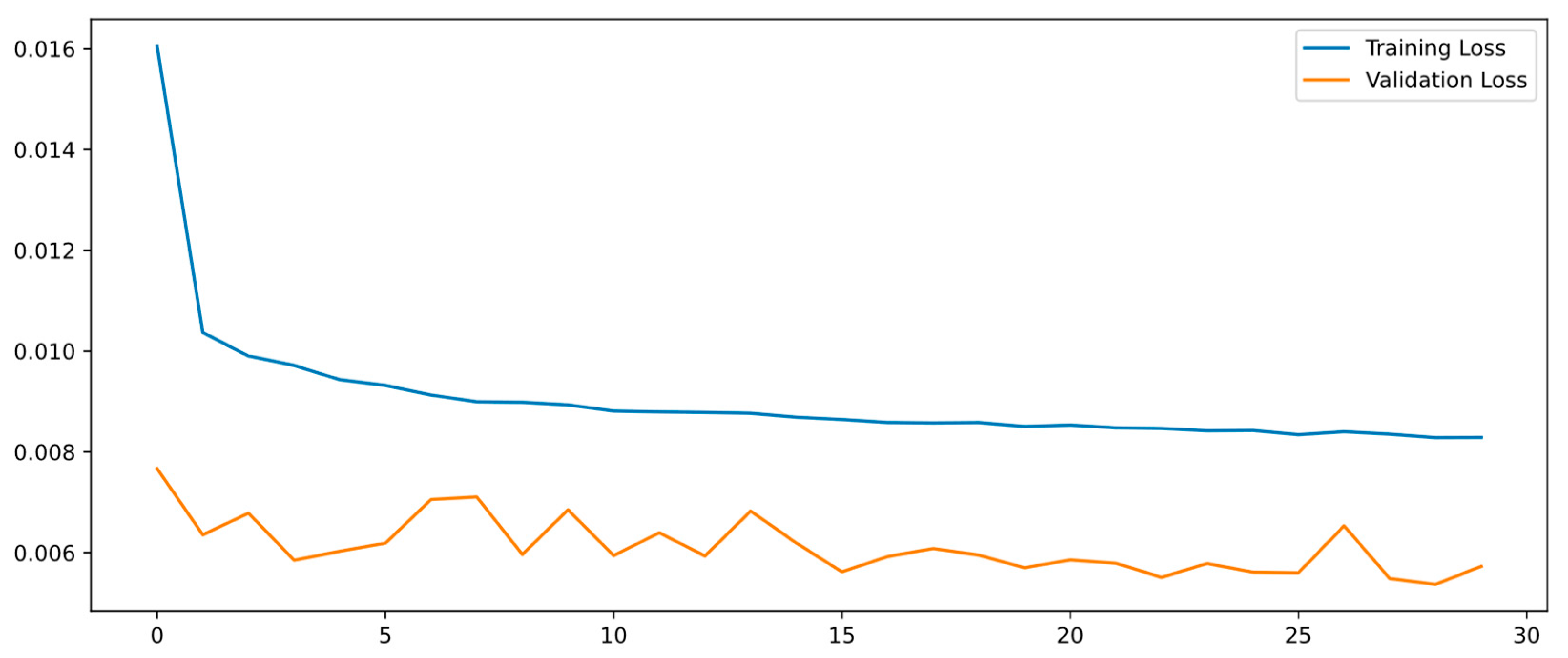
4.2. Training and Testing Details

Before the features can be utilized for model training, the data must first go through the data preparation process. This process includes noise removal, the rescaling of data, and data reframing, in which data cells with null or invalid information are removed. Subsequently, all datasets are rescaled in the range of [0, 1] to boost the performance of the model and are then reframed into a time series metric, as shown in Equation (4).
The GCMN model in this case study has a training and testing element, where the projected outcomes from the training aspect are compared to the testing data to assess the model’s performance. To train and evaluate the GCMN model, the prepared data was separated, reorganized, and restructured into two matrix groups. In particular, the first 80% of the dataset are regards as training data and the remaining 20% are utilized to evaluate the model’s performance. The GCMN model is composed of two GCN layers followed by two LSTM layers with the number of nodes being 16, 10, 256, and 256 in each layer, respectively. The activation functions for the GCN and LSTM layers are ReLU and ELU, respectively. To compile the established model, Adam was selected as the optimizer, MAE was utilized as the loss function, and MSE was the evaluation metric. A detailed hyperparameter selection and a summary of the GCMN model are listed in Table 3 and Table 4, respectively. To generate the prediction results, the model was trained employing a batch size of 15 and for 30 epochs as illustrated in the model’s summary in Table 4.
As discussed in the previous section, the GCMN model employs a time series prediction technique, which includes historical data from timesteps  t n  to t for each input variable,  x 1  to  x 10  in the training and testing process. Moreover, without considering the current timestep, the historical data of the output variable,  y  from timestep  t n  to  t 1  is incorporated in the training and testing procedure, where n is the number of historical timesteps involved for the model training and testing. For illustration purposes, the training and validation loss during the training of the GCMN model with input from timesteps from  t 2  is shown in Figure 7. In essence, the value of training loss function declines significantly in the first 5 epochs and begins to normalize afterward. The loss function converges to the lowest with slight local oscillations as the number of training epochs exceeds 25, indicating that the proposed 30 number of epochs are sufficient for the model to achieve its best performance. In addition, the loss function for each output starts at less than 0.016, where the low errors demonstrate the model’s great ability to map nonlinear relationships between input and output variables.

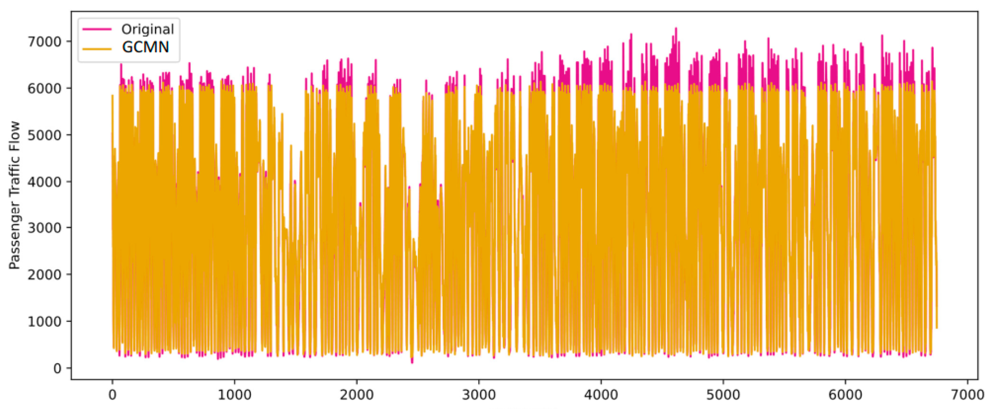
4.3. Analysis of Results

The performance of the proposed method was evaluated by comparing the prediction results with the ground truth values from  X t e s t . Common statistical criteria including MAE, RMSE, and  R 2  were employed to identify and analyze the validity of the produced model’s performance.
This model provides an accurate estimation of traffic flow. Refer to Table 5 for the results of MAE, RMSE, and  R 2  produced by the model. Despite the selection of the timesteps, the model generates an average MAE of 368.364, RMSE of 549.527, and R2 of 0.920. Considering the data scale in Table 2, in which the traffic flow varies from 0 to 7280, the error is considered very low. In addition, a high value of  R 2  is a good indication that the predicted values fit well with the ground truth. The result is also reflected in Figure 8, where the line plots of ground truth and predicted values are presented. Generally, the predicted values closely follow the trends of the ground truth, which indicates the high accuracy of the proposed method. Another point worth mentioning is the training and prediction time for the model. As shown in Table 5, the average training time for the model is 29.14 s per epoch, which indicates the model can be trained in about 15 min given that 30 epochs are needed. However, since the prediction can be done almost immediately when the inputs are provided, the model can be effectively implemented for the real-time estimation of traffic flow.
Timestep  t 2  is the most suitable historical timestep as the input. Table 5 shows the results of the constructed model for MRS passenger traffic flow using time series data from  t  to  t 7 ; revealing that despite utilizing more historical data in timesteps  t 3  to  t 7 , the results slightly dropped and ceased rising in general. Furthermore, the  R 2 , MAE, and RMSE for  t 3  deteriorated slightly despite its computational time increasing from  t 2 . Therefore, the overall better results are shown in  t 2  as it also has a shorter computational time compared with  t 3  to   t 7  with similar results. Additionally, using time series of up to  t 2  as compared to  t 1 , MAE, RMSE, and  R 2  all improved slightly. With the  R 2  of 0.930 for passenger traffic flow as seen in Table 5 below, this would mean that the predicted results forecasted  X t e s t  with 93.0%. Hence, timestep  t 2  produces the best overall results in terms of MAE, RMSE, R2 and average time and will be used in the following sections. Figure 8 below plots the comparison between the predicted values and  X t e s t  showing detailed results for passenger traffic flow.

5. Discussion

Although the results of the case study demonstrate the effectiveness of the proposed model, it is worth comparing it with state-of-the-art methods for further validation. Therefore, two alternative predictive models, LSTM and light gradient boosting machine (LightGBM), are appointed, as both have been extensively utilized for traffic flow prediction. For instance, Latifa et al. [31] predict the train delay using the LightGBM method. Jiang et al. [32] adopted LightGBM to estimate pedestrian volume in urban areas. Similarly, LSTM has been investigated by many scholars for traffic-related studies.
For a fair comparison, the models were trained by the same dataset. The hyperparameter settings for the LSTM model and the LightGBM model are shown in Table 6 and Table 7, respectively. The deep learning LSTM metamodel predicts passenger traffic flow using data from two timesteps of each predictive variable using an LSTM network with two LSTM layers of 256 nodes each, with the activation function ELU and loss function MSE using Adam as the optimizer. In the LightGBM model, the candidate values for maximum depth, number of leaves, learning rate, and number of estimators are set to 7, 10, 0.1, and 80, respectively. This hyperparameter configuration of the LSTM model is compatible with the LSTM component of the GCMN model for a more accurate analysis.
Table 8 and Table 9 describe the prediction results of the developed model for passenger traffic flow using the time series data of  t  to  t 2  in Table 8 and  t  to  t 1  in Table 9 to compare the LSTM model, LightGBM model, and GCMN developed model by evaluating values from the prediction results against the test data based on common evaluation metrics: MAE, RMSE, and  R 2 . As shown in Table 9, for the timestamp  t 2 , the MAE, RMSE, and  R 2  for the passenger traffic flow of the GCMN model are slightly better than those of the LSTM model and LightGBM model, with  R 2  of 0.930 for the GCMN model,  R 2  of 0.925 for the LGBM model, and  R 2  of 0.915 for the LSTM model, which corresponds to 93.0% for the developed model, 92.5% for the LightGBM model, and 91.5% for the LSTM model. Similarly, the MAE and RMSE values of the GCMN are also better than those of the LightGBM model and LSTM model with 339.889, 358.477, and 383.446, respectively, for MAE and 510.627, 535.749, and 570.601, respectively, for RMSE for timestamp  t 2 . Table 8 shows that for timestamp  t 1 , the MAE, RMSE, and  R 2  of GCMN are still better than those of the LSTM model despite both being poorer than its  t 2  timestep values. This demonstrates that the generated GCMN model’s predicted results are more accurate than those of the LSTM model and LGBM model for passenger traffic flow prediction. Additionally, the comparison between the predicted values and ground truth generated by the GCMN model, LightGBM model, and LSTM model under the time step of  t 1  are shown in Figure 9, below. Generally, the result from the line plots is consistent with the evaluation metrics, where the prediction of GCMN is closer than that of the state-of-the-art methods.
With the prediction of passenger traffic flow, the model would be able to aid in the evaluation and management of future MRS planning and upgrading works by metro owners and architects by controlling passenger traffic flow, especially during high peak hours beforehand to reduce metro passenger traffic flow volume, resulting in more efficient mobility and shorter waiting times, thus ensuring user satisfaction and technology acceptance in terms of robustness, reliability, and capacity to have an effective method for traffic management and control.

6. Conclusions and Future Works

This study establishes a hybrid deep learning model for the accurate estimation of passenger traffic flow. By integrating the GCN and LSTM cells, a hybrid model GCMN is created which can extract useful features from the historical data of the traffic flow and weather factors. The developed approach can be employed as a useful tool to assist the metro railway industry in countries with metropolitan cities to improve MRS performance.
To demonstrate the effectiveness of the developed approach, real data from Delhi’s metro system were employed as a case study with a total of 10 attributes utilized as input parameters, and passenger traffic flow was utilized as an output parameter in this prediction model. The results from this case study indicate the following: (1) The developed method achieves an accurate real-time estimation for passenger traffic flow with 339.889 for MAE, 510.627 for RMSE, and 0.930 for  R 2 . (2) The prediction accuracy is highest when the timestep is  t 2  with MAE and RMSE being at their lowest and  R 2  being at its highest for this timestep as compared to the other timesteps with the shortest computation times. (3) The proposed method achieves higher prediction accuracy compared with state-of-the-art methods, being 0.54% and 1.64% better than the LightGBM and LSTM, respectively, in terms of R2.
In spite of the fact that the hybrid model has excellent performance results, it still has certain limitations. For this study, all input factors were numerical, while some categorical data (e.g., weather conditions) were not considered. Future studies may consider including these categorical data as the inputs, which has the potential to further improve prediction accuracy.

Author Contributions

Conceptualization, S.P. and L.Z.; methodology, S.P. and L.Z.; validation, L.Z.; formal analysis, S.P. and L.Z.; data curation, X.F. and L.Z.; writing—original draft preparation, X.F. and S.P.; writing—review and editing, X.F., L.Z. and M.W.; visualization, X.F., L.Z. and M.W.; supervision, L.Z.; project administration, L.Z.; funding acquisition, L.Z. All authors have read and agreed to the published version of the manuscript.

Funding

This work is supported in part by the National Natural Science Foundation of China (No. 71171101), the Outstanding Youth Fund of Hubei Province (No. 2022CFA062), and the Start-Up Grant at Huazhong University of Science and Technology (No. 3004242122).

Data Availability Statement

The data used in this study was extracted from Kaggle (see the link https://www.kaggle.com/datasets/umairnsr87/indian-metro-data).

Conflicts of Interest

The authors declare no conflict of interest.

References

  1. Lowe, M.D. Alternatives to the automobile: Transport for livable cities. Ekistics 1990, 269–282. [Google Scholar]
  2. Li, Q.Y.; Zhong, Z.D.; Liu, M.; Fang, W.W. Smart railway based on the Internet of Things. In Big Data Analytics for Sensor-Network Collected Intelligence; Academic Press: Amsterdam, The Netherlands, 2017; pp. 280–297. [Google Scholar]
  3. Lv, Y.; Duan, Y.; Kang, W.; Li, Z.; Wang, F.-Y. Traffic Flow Prediction with Big Data: A Deep Learning Approach. IEEE Trans. Intell. Transp. Syst. 2015, 16, 865–873. [Google Scholar] [CrossRef]
  4. Sajanraj, T.D.; Mulerikkal, J.; Raghavendra, S.; Vinith, R.; Fábera, V. Passenger flow prediction from AFC data using station memorizing LSTM for metro rail systems. Neural Netw. World 2021, 31, 173–189. [Google Scholar] [CrossRef]
  5. Yoo, S.; Kim, H.; Kim, W.; Kim, N.; Lee, J. Controlling passenger flow to mitigate the effects of platform overcrowding on train dwell time. J. Intell. Transp. Syst. 2020, 26, 366–381. [Google Scholar] [CrossRef]
  6. Mulerikkal, J.; Thandassery, S.; Rejathalal, V.; Kunnamkody, D.M.D. Performance improvement for metro passenger flow forecast using spatio-temporal deep neural network. Neural Comput. Appl. 2021, 34, 983–994. [Google Scholar] [CrossRef]
  7. Garber, N.J.; Hoel, L.A. Traffic and Highway Engineering; Cengage Learning: Boston, MA, USA, 2019. [Google Scholar]
  8. Nihan, N.L.; Kjell, O.H. Use of the Box and Jenkins time series technique in traffic forecasting. Transportation 1980, 9, 125–143. [Google Scholar] [CrossRef]
  9. Sun, H.; Liu, H.; Xiao, H.; He, R.R.; Ran, B. Use of Local Linear Regression Model for Short-Term Traffic Forecasting. Transp. Res. Rec. J. Transp. Res. Board 2003, 1836, 143–150. [Google Scholar] [CrossRef]
  10. Boukerche, A.; Wang, J. Machine Learning-based traffic prediction models for Intelligent Transportation Systems. Comput. Networks 2020, 181, 107530. [Google Scholar] [CrossRef]
  11. Castillo, E.; Menéndez, J.M.; Sánchez-Cambronero, S. Predicting traffic flow using Bayesian networks. Transp. Res. Part B Methodol. 2008, 42, 482–509. [Google Scholar] [CrossRef]
  12. Hong, W.-C.; Ping-Feng, P.; Shun-Lin, Y.; Robert, T. Highway traffic forecasting by support vector regression model with tabu search algorithms. In Proceedings of the 2006 IEEE International Joint Conference on Neural Network Proceedings, Vancouver, BC, Canada, 16–21 July 2006; pp. 1617–1621. [Google Scholar]
  13. Zhao, L.; Song, Y.; Zhang, C.; Liu, Y.; Wang, P.; Lin, T.; Deng, M.; Li, H. T-GCN: A Temporal Graph Convolutional Network for Traffic Prediction. IEEE Trans. Intell. Transp. Syst. 2019, 21, 3848–3858. [Google Scholar] [CrossRef] [Green Version]
  14. Fu, X.; Wu, M.; Ponnarasu, S.; Zhang, L. A hybrid deep learning approach for dynamic attitude and position prediction in tunnel construction considering spatio-temporal patterns. Expert Syst. Appl. 2023, 212, 118721. [Google Scholar] [CrossRef]
  15. Chen, C.-F.; Chang, Y.-H. Seasonal ARIMA forecasting of inbound air travel arrivals to Taiwan. Transportmetrica 2009, 5, 125–140. [Google Scholar] [CrossRef]
  16. Hamed, M.M.; Al-Masaeid, H.R.; Said, Z.M.B. Short-Term Prediction of Traffic Volume in Urban Arterials. J. Transp. Eng. 1995, 121, 249–254. [Google Scholar] [CrossRef]
  17. Crawford, F.; Watling, D.; Connors, R. A statistical method for estimating predictable differences between daily traffic flow profiles. Transp. Res. Part B Methodol. 2017, 95, 196–213. [Google Scholar] [CrossRef] [Green Version]
  18. Polson, N.G.; Vadim, O.S. Deep learning for short-term traffic flow prediction. Transp. Res. Part C Emerg. Technol. 2017, 79, 1–17. [Google Scholar] [CrossRef] [Green Version]
  19. Nie, L.; Jiang, D.; Guo, L.; Yu, S. Traffic matrix prediction and estimation based on deep learning in large-scale IP backbone networks. J. Netw. Comput. Appl. 2016, 76, 16–22. [Google Scholar] [CrossRef]
  20. Ma, X.; Tao, Z.; Wang, Y.; Yu, H.; Wang, Y. Long short-term memory neural network for traffic speed prediction using remote microwave sensor data. Transp. Res. Part C Emerg. Technol. 2015, 54, 187–197. [Google Scholar] [CrossRef]
  21. Chen, H.; Grant-Muller, S. Use of sequential learning for short-term traffic flow forecasting. Transp. Res. Part C Emerg. Technol. 2001, 9, 319–336. [Google Scholar] [CrossRef]
  22. Chiang, W.-C.; Russell, R.A.; Urban, T.L. Forecasting ridership for a metropolitan transit authority. Transp. Res. Part A Policy Pr. 2011, 45, 696–705. [Google Scholar] [CrossRef]
  23. Tan, M.-C.; Wong, S.C.; Xu, J.-M.; Guan, Z.-R.; Zhang, P. An Aggregation Approach to Short-Term Traffic Flow Prediction. IEEE Trans. Intell. Transp. Syst. 2009, 10, 60–69. [Google Scholar]
  24. Tsai, T.-H.; Lee, C.-K.; Wei, C.-H. Neural network based temporal feature models for short-term railway passenger demand forecasting. Expert Syst. Appl. 2009, 36, 3728–3736. [Google Scholar] [CrossRef]
  25. Sedgwick, P. Pearson’s correlation coefficient. BMJ 2012, 345, e4483. [Google Scholar] [CrossRef] [Green Version]
  26. Obilor, I.E.; Amadi, C.E. Test for significance of Pearson’s correlation coefficient. Int. J. Innov. Math. Stat. Energy Policies 2018, 6, 11–23. [Google Scholar]
  27. Runge, J. Discovering contemporaneous and lagged causal relations in autocorrelated nonlinear time series datasets. In Proceedings of the Conference on Uncertainty in Artificial Intelligence, Online, 4–6 August 2020; pp. 1388–1397. [Google Scholar]
  28. Runge, J. Causal Inference and Complex Network Methods for the Geosciences. Available online: https://jakobrunge.github.io/tigramite/ (accessed on 28 September 2017).
  29. Krupenevich, R.L.; Funk, C.J.; Franz, J.R. Automated analysis of medial gastrocnemius muscle-tendon junction displacements in heathy young adults during isolated contractions and walking using deep neural networks. Comput. Methods Programs Biomed. 2021, 206, 106120. [Google Scholar] [CrossRef]
  30. “Delhi Metro Route Map, Timings, Lines, Facts—Fabhotels.” FabHotels Travel Blog. Available online: https://www.fabhotels.com/blog/indian-metro-rail-networks/delhi-metro/ (accessed on 3 March 2022).
  31. Laifa, H.; Ghezalaa, B.H.H. Train delay prediction in Tunisian railway through LightGBM model. Procedia Comput. Sci. 2021, 192, 981–990. [Google Scholar] [CrossRef]
  32. Jiang, F.; Ma, J.; Li, Z. Pedestrian volume prediction with high spatiotemporal granularity in urban areas by the enhanced learning model. Sustain. Cities Soc. 2021, 79, 103653. [Google Scholar] [CrossRef]
Figure 1. Framework of the developed GCMN approach.
Buildings 13 01514 g001
Figure 2. Conceptual diagram of the causal network discovery.
Buildings 13 01514 g002
Figure 3. Structure of the LSTM cell.
Buildings 13 01514 g003
Figure 4. Structure of a typical GCN layer and hidden layers.
Buildings 13 01514 g004
Figure 5. Structure of GCMN cell with the combination of LSTM and GCN.
Buildings 13 01514 g005
Figure 6. Triangle correlation map of different variables.
Buildings 13 01514 g006
Figure 7. Curve of loss function of training and test sets of GCMN model for  t 2 .
Buildings 13 01514 g007
Figure 8. Results of predictions and ground truth using the GCMN model.
Buildings 13 01514 g008
Figure 9. Results of predictions and ground truth using LSTM, LGBM, and GCMN.
Buildings 13 01514 g009
Table 1. Description of input and output variables of the prediction model.
ParameterSymbolDescription
Air Pollution Index x 1 Air quality index that ranges from 10 to 300
Humidity x 2 General humidity measured in Celsius
Wind Speed x 3 Wind speed is measured in miles per hour
Wind Direction x 4 Cardinal wind direction (0 to 360 degrees)
Visibility in Miles x 5 Visibility of distance in miles
Dew Point x 6 Dew point measured in Celsius
Temperature x 7 Average national temperature measured in Kelvin
Rain Per Hour x 8 Amount of rainfall measured in millimeters in an hour
Snow Per Hour x 9 Amount of snowfall measured in millimeters in an hour
Clouds All x 10 Percentage of cloud cover in the sky
Passenger Traffic Flow y Numeric hourly traffic volume bound in a specific direction at the urban railway system
Table 2. Data description for the key traffic parameters.
FactorCountMeanStdMinMax
x 1 33,750154.8483.7310.0299.0
x 2 33,75071.2116.8513.0100.0
x 3 33,7503.382.06016.0
x 4 33,750199.4799.840360.0
x 5 33,7504.992.571.09.0
x 6 33,7504.992.571.09.0
x 7 33,750280.0713.420308.24
x 8 33,7500.44953.5309831.30
x 9 33,7500.000320.009800.510
x 10 33,75050.4638.870100.0
y 33,7503240.121991.4607280.0
Table 3. The hyperparameter setting of GCMN.
Parameter TypeSetting
GCN ActivationReLU
LSTM ActivationELU
Epochs30
Batch Size10
Loss FunctionMAE
OptimizersAdam
MetricsMSE
Table 4. Summary of GCMN model structure.
LayerTypeOutput ShapeParameter
1GCN(None, 32, 16)2986
2GCN(None, 32, 10)3130
3LSTM(None, 10, 256)318,464
4LSTM(None, 256)525,312
5Dense(None, 32)13,878
Table 5. Results of  R 2 , MAE, RMSE, and average time of prediction results for GCMN model of output variables for  t 1  to  t 7 .
Metric t 1 t 2 t 3 t 4 t 5 t 6 t 7 Average
R20.8800.9300.9190.9290.9300.9280.9270.920
MAE489.922339.889364.451342.571340.784349.806351.126368.364
RMSE672.406510.627554.765523.717512.702533.192539.283549.527
Average Time 16   s / epoch 20   s / epoch 27   s / epoch 30   s / epoch 34   s / epoch 37   s / epoch 40   s / epoch 29.14   s / epoch
Table 6. Parameter setting of LSTM metamodel.
Parameter TypeSetting
LSTM ActivationELU
Epochs30
Batch Size15
Loss FunctionMSE
OptimizersAdam
Table 7. Candidate values setting for LGBM metamodel parameters.
Parameter TypeCandidate Values X 11
Maximum Depth ( D m ) 2 ,   3 ,   4 ,   5 ,   6 ,   7 ,   8 ,   9 7
Number of Leaves ( N l ) 5 ,   10 ,   15 ,   20 ,   25 ,   30 10
Learning Rate ( η ) 0.05 ,   0.1 ,   0.15 0.1
Number of Estimators ( λ ) 50 ,   60 ,   70 ,   80 ,   90 ,   100 80
Table 8. Comparison with LSTM and LGBM for  t 1 .
t 1 LSTMLGBMGCMN
R 2 0.8510.8720.880
MAE527.608502.974489.922
RMSE754.067698.095672.406
Table 9. Comparison with LSTM and LGBM for  t 2 .
t 2 LSTMLGBMGCMN
R 2 0.9150.9250.930
MAE383.446358.477339.889
RMSE570.601535.749510.627
Disclaimer/Publisher’s Note: The statements, opinions and data contained in all publications are solely those of the individual author(s) and contributor(s) and not of MDPI and/or the editor(s). MDPI and/or the editor(s) disclaim responsibility for any injury to people or property resulting from any ideas, methods, instructions or products referred to in the content.

