Article

Comparative Analysis of ANN and LSTM Prediction Accuracy and Cooling Energy Savings through AHU-DAT Control in an Office Building

1
College of Design, North Carolina State University, Raleigh, NC 27695, USA
2
Buildings and Transportation Science Division, Oak Ridge National Laboratory, Oak Ridge, TN 37830, USA
3
School of Architecture, Korea University, Seoul 02481, Republic of Korea
*
Author to whom correspondence should be addressed.
These authors contributed equally to this work.
Buildings 2023, 13(6), 1434; https://doi.org/10.3390/buildings13061434
Submission received: 27 April 2023 / Revised: 19 May 2023 / Accepted: 26 May 2023 / Published: 31 May 2023
(This article belongs to the Special Issue Advanced Building Technologies for Energy Savings and Decarbonization)

Abstract

:
This paper proposes the optimal algorithm for controlling the HVAC system in the target building. Previous studies have analyzed pre-selected algorithms without considering the unique data characteristics of the target building, such as location, climate conditions, and HVAC system type. To address this, we compare the accuracy of cooling load prediction using ANN and LSTM algorithms, widely used in building energy research, to determine the optimal algorithm for HVAC control in the target building. We develop a simulation model calibrated with actual data to ensure data reliability and compare the energy consumption of the existing HVAC control method and the two algorithms-based methods. Results show that the ANN algorithm, with a CV(RMSE) of 12.7%, has a higher prediction accuracy than the LSTM algorithm, CV(RMSE) of 17.3%, making it a more suitable algorithm for HVAC control. Furthermore, implementing the ANN-based approach results in a 3.2% cooling energy reduction from the optimal control of Air Handling Unit (AHU) Discharge Air Temperature (DAT) compared to the fixed DAT at 12.8 °C in a representative day. This study demonstrates that ML-based HVAC system control can effectively reduce cooling energy consumption in HVAC systems, providing an effective strategy for energy conservation and improved HVAC system efficiency.

1. Introduction

1.1. Background

According to the Annual Energy Outlook 2019 published by the U.S. Energy Information Administration (EIA), the building sector accounts for 40% of the total energy consumed in the United States. Commercial buildings constitute about 50% of total energy consumption, of which about 40% is used for heating, ventilating, and air conditioning (HVAC) [1]. The International Energy Agency (IEA) report “The Future of Cooling” affirmed that global energy demand and district cooling and heating demand had increased rapidly over the past decade due to economic development—electricity energy consumption for space cooling accounts for about 20% of total building energy. In addition, the report emphasized that if space cooling systems remain inefficient, global cooling energy demand will be three times higher in 2050 than in 2016 [2].
High-efficiency cooling systems or optimal control of cooling systems should be considered to increase cooling system efficiency. High-efficiency cooling systems are suitable for newly built buildings but are challenging to apply in existing buildings due to the cost and time required for system replacement. Therefore, to increase the efficiency of cooling systems already installed in existing buildings, the better option is to ensure their optimal control [3].
Various studies on optimal control methods for HVAC systems have used advanced technology, such as machine learning (ML)-based controls [3,4,5]. Based on their learning method, ML methods are generally categorized into three main types: supervised learning, semi-supervised learning, and unsupervised learning. The selection of the learning method primarily depends on the intended purpose. For tasks involving regression, such as prediction and control, a supervised learning-based algorithm is generally suitable [3,4,5]. Artificial neural networks (ANNs), particularly those that imitate the human brain, and Long Short-Term Memory (LSTM) algorithms specialized in time series data are widely utilized as the primary algorithms in supervised learning [5,6,7,8,9,10,11,12,13,14,15,16,17,18,19].
Previous studies have utilized ANN and LSTM algorithms to predict building energy consumption, cooling and heating load, and control HVAC systems. Using an ANN-based prediction model, Lee et al. measured the cooling energy reduction effect during summer according to Air Handling Unit (AHU) optimal temperature control. The research results showed that compared to a conventional control method, the ANN-based predictive control method could reduce cooling energy consumption by approximately 10%. The authors argued that the ANN-based control algorithm could be applied to various forced air systems by taking dynamic operating conditions [5]. Qian et al. asserted that accurate HVAC system load forecasting is required for optimal control and design. They developed an ANN-based load forecasting model and analyzed its accuracy. The proposed model showed 10% more accuracy than the conventional load forecasting method [6].
Moon et al. developed an ANN-based Variable Refrigerant Flow system control algorithm to increase the cost-effectiveness in the heating season. Comparing simulation results with ANN prediction results, they found that the ANN model has a coefficient of variation root mean square error (CV[RMSE]) of 7.42%. The ANN model was embedded in the control algorithm to determine the intermittent operation. They confirmed that the ANN model and the control algorithm could enhance the prediction accuracy and cost-effectiveness of the heating system [7]. Park et al. proposed an ANN-based prediction model to forecast the energy cost for a VRF heating system. In the performance evaluation, the prediction accuracy of the proposed model was within the recommended level, with a coefficient of variation root mean square error of 4.87%. They suggested that the predicted energy cost can be used as a determinant for the control algorithm to reduce operating costs [8]. Mtibaa et al. developed an LSTM-based model predictive control method. The prediction model was used for energy consumption, peak demand, and indoor thermal discomfort during occupied hours. The results showed that the LSTM model reduced energy consumption and indoor thermal discomfort degree [9].
Sendra-Arranz and Gutierrez stated that the HVAC system predictive control is essential to realize demand-side management strategies. They developed an LSTM-based prediction model to forecast a day ahead of the energy consumption of an HVAC system. The model showed outstanding results, supported by a Pearson test correlation coefficient 0.972 and a normalized root mean square error of 0.052 [10]. Mba et al. conducted a study to predict room temperature and humidity in the past using ANN to reduce cooling energy in residential buildings. The ANN model showed 98% accuracy [11]. Zhao and Liu proposed a load-predicting method for office buildings based on regression analysis and artificial intelligence [12]. Afram et al. studied ANN-based HVAC optimal control in residential buildings. They found that HVAC operation costs can be lowered using the proposed ANN-based HVAC control strategy [13]. Jang et al. developed an LSTM-based prediction model to predict the heating energy consumption in daycare centres. They used environmental data and building operation pattern data to train the LSTM model. The optimized LSTM model showed a CV(RMSE) of 17.6% during the winter season [14]. Faid et al. proposed prediction models based on LSTM, support vector regression, and Gaussian process regression to predict the peak electricity usage of a target building. The electricity usage included the electric equipment and HVAC systems energy consumption of the building. They found that the LSTM model showed the highest accuracy among the three models. However, they cited the need for massive time series data as a drawback of LSTM models [15]. Fang et al. developed an LSTM-based prediction model to determine the accurate indoor temperature for controlling the HVAC system [16]. Bouktif et al. constructed a model for predicting short- and mid-term building electric loads using the LSTM algorithm and established that the proposed LSTM model has high accuracy [17].
Similarly, Somu et al. developed an LSTM model to predict building energy consumption. Their proposed model also showed high accuracy [18]. Peng et al. claimed that their LSTM model demonstrates high efficiency in building load forecasting [19].
In summary, many previous studies have analyzed pre-selected algorithms without considering the data characteristics of the target building. However, many factors influence building loads, such as location, climate conditions, and HVAC system type. It is, therefore, crucial to carefully select an appropriate algorithm that considers the specific characteristics of the target building. Furthermore, ensuring the reliability of the findings was challenging in certain studies because simulations were not calibrated with actual building data. To achieve reliable algorithm-based HVAC control, it is imperative to establish the credibility of the algorithm. Ensuring the reliability of actual HVAC control is crucial, even if predictions are accurate in an ideal environment. The use of unverified data can undermine this reliability. Therefore, utilizing a calibrated model based on the actual data is essential. In this study, we address this concern by developing a calibrated simulation model, which enhances the reliability of the data used.
Our research objective is to determine the optimal algorithm for HVAC system control in the target building. To achieve this, we compare the accuracy of cooling load prediction using two widely utilized algorithms in building energy research: ANN and LSTM. Additionally, we investigate the impact of cooling load prediction accuracy on HVAC control by comparing the patterns of AHU discharge air temperature (DAT) control values. We select the most suitable ML algorithm for the target building based on these comparisons. Furthermore, we evaluate the feasibility of applying ML-based HVAC control by selecting representative dates for analysis.

1.2. Scope

This study aims to find the optimal algorithm for HVAC system control in the target building. We used Python programming to develop prediction models using ANN and LSTM algorithms. To train and test two models, we utilized an EnergyPlus simulation model calibrated by the actual data. We compared the accuracy of the prediction models and then conducted a comparative analysis of AHU-DAT patterns to determine the optimal algorithm for HVAC control in the target building. In addition, we performed a feasibility analysis by analyzing a representative day to assess the potential for ML-based HVAC control in the target building. A visual representation of our process can be found in Figure 1.

2. Machine Learning-Based Prediction Model: Concept and Formulation

2.1. Artificial Neural Network

Figure 2 shows the structure of an ANN algorithm with an input layer, a hidden layer, and an output layer. In the following paragraphs, we explain the process and outline the formulas related to the learning method of ANN.
The critical advantage of ANN is its robustness to noisy input data. They can learn to generalize from training examples and make accurate predictions even in noise [3,4,5,6,7,8,9,10,11,12]. However, a limitation of ANN is that they are not inherently designed to capture temporal dependencies in sequential data. They treat all inputs independently, which can be a drawback in tasks where the order or timing of the data is essential [3,4,5,6,7,8,9,10,11,12].
First, ANN prints a predicted value through a certain calculation process in the input, hidden, and output layers based on the input data using feed-forward propagation. After which, it performs an error back-propagation process to identify the error between the predicted value and the correct determined value, which is then reflected in the next learning.
The feed-forward neural network, the basic algorithm of ANN, is transmitted from the input layer and the hidden layer to the output layer. Each layer consists of nodes, and each node is connected. When neurons in the input layer receive an external input, weight factors are applied to input data and output values through the activation function. Equations (1) and (2) [4,20] are the formulas used for data forward propagation in ANN, using sigmoid as an activation function [4,20].
y = σ b + i = 1 n x i w i
where
y = output of the node,
σ = sigmoid function,
b = bias,
n = number of nodes in a previous layer connected to the node,
x i = input values of nodes in a previous layer connected to the node, and
w i = weight factor of all nodes connected to the node.
σ = 1 1 + e x
where
x = a value obtained by adding a bias to the value multiplied by all input values input to the node and a weight factor.
When an error occurs in the resulting data, updating the weight factor by propagating the error to the previous layer is repeated. This process is called back-propagation. The optimal value is found by updating the weight factor during the back-propagation process by repeating the gradient descent method. This process also minimizes the error rate of the ANN model and increases the prediction accuracy of printed data.
Equations (3)–(6) are the formulas used for updating the weight factor through the gradient descent method [20]. Equation (3) is the final formula for calculating the error function for the weight factor of each node located between the hidden layer and the output layer [20].
E w h o = t o o o × s i g m o i d ( h w h o × o h ) ( 1 s i g m o i d ( h w h o × o h ) ) × o h
where
E w h o = slope of the error for the weight factor located between the hidden layer and the output layer,
t o o o = difference between the printed values and the correct answer,
s i g m o i d h w h o × o h = sum of the input values coming in the node located in the output layer, and
o h = output value of the node located in the hidden layer.
Equation (4) is the formula for updating the weight factor between the hidden and output layers based on the calculated error function [20]. The updated weight factor can be calculated by subtracting the value obtained and multiplying the error slope calculated in Equation (6) by a constant from the previous value of the weight factor. The constant α adjusts the intensity of the change, which is called the learning rate [4,20].
N e w   w h o = O l d   w h o α   E w h o
where
w h o = weight factor between the hidden layer and the output layer,
α = learning rate, and
E w h o = slope of the error for the weight factor between the hidden and output layers.
Equation (5) is the final formula for calculating the error function for the weight factor of the nodes between the input and hidden layers [20].
E w i h = e h × s i g m o i d ( i w i h × o i ) ( 1 s i g m o i d ( i w i h × o i ) ) × o i
where
E w i h = slope of the error for the weight factor between the input layer and the hidden layer,
e h = back-propagation error transmitted to the hidden layer,
s i g m o i d i w i h × o i = sum of the input values from the input layer to the node located in the hidden layer, and
o i = output of the node in the input layer.
Equation (6) is the formula for updating the weight factor located between the input layer and the hidden layer based on the calculated error function [20].
N e w   w i h = O l d   w i h α   E w i h
where
w i h = weight factor between the input layer and hidden layer,
α = learning rate, and
E w i h = slope of the error for the weight factor between the input layer and hidden layer.

2.2. Long Short-Term Memory

Long Short-Term Memory is an algorithm that compensates for the shortcomings of RNN. RNN was introduced in the study of David Rumelhart in 1986. It is a type of ANN characterized as having an internal circular structure of data [21]. It involves saving previous data and feeding it back when inputting new data so it is not forgotten. Unlike ANN, where all input data are independent, RNN processes input data in its internal memory so that all input values are related [22]. As such, RNN is suitable for learning time series data with temporal correlation [23].
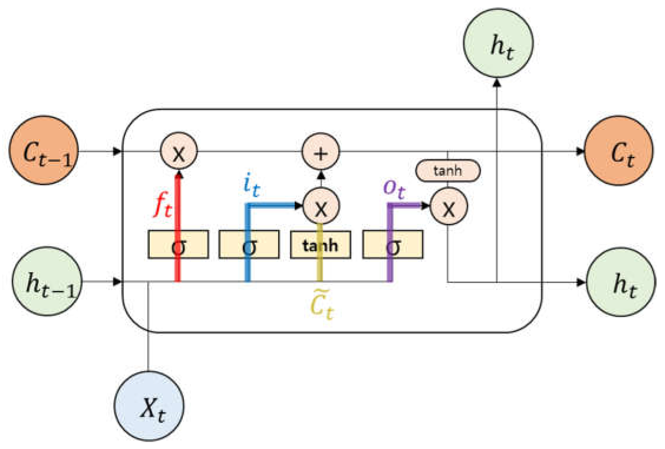
In addition, RNN uses “back-propagation through time” during training, performing back-propagation of errors up to the earliest time step for every time step [24]. If the time step exceeds a certain period of time, gradient vanishing can occur in which the learning rate is not updated, and long-term patterns cannot be learned [23]. To overcome these shortcomings of RNN, Sepp Hochreiter and Jürgen Schmidhuberdm introduced LSTM in 1997 [22]. Figure 3 shows the structure of LSTM.
The LSTM structure, as shown in Figure 3, is designed to continuously transmit information necessary for long-term learning by improving the existing RNN structure. Learning is performed on time-dependent data input through a long-term memory device called cell state—the core of LSTM. In LSTM, a forget gate, an input gate, a hidden state, and an output gate are added to the existing RNN memory cell. The role of the forget gate and input gate is to update the value of the cell state. Meanwhile, the hidden state and the output gate’s role is to print a predicted value based on the updated cell state value and input value.
LSTM has a key advantage in that it is specifically designed to model and capture long-term dependencies in sequential data [14,15,16,17,18,19]. With a memory cell that can store information over extended time intervals, LSTM is effective in tasks involving time series analysis, natural language processing, and speech recognition [25]. However, a significant drawback of LSTM is its higher computational cost than ANN [23].
The learning method of LSTM entails several formulas. Equations (7)–(11) calculate the forget gate and input gate to update the cell state [25]. The forget gate calculates a value based on the input data of the current time step and the predicted value of LSTM in the previous time step. The value calculated for the forget gate is then multiplied by the cell state value of the previous time step. The output value of LSTM in the previous time step and the input data in the current time step helps determine if the value of the cell state in the previous time step needs to be reduced through the forget gate.
Equation (7) is the formula for the forget gate [25].
f t = σ   W f h t 1 , x t + b f
where
f t = output of the forget gate,
σ = sigmoid function,
W f = weight factor assigned to the forget gate,
h t 1 = output value of LSTM in the previous time step,
x t = input data in the current time step, and
b f = bias assigned to the forget gate.
The input gate plays a role in determining how much new information is stored in the cell state. First, the input gate calculates the output value of the input gate using Equation (8) and determines new values that can be added to the cell state using Equations (9) and (10) [25]. After which, Equations (8) and (9) are multiplied to output one value [25]. This value is then added to the updated cell state value through the forget gate to determine the cell state value of the current time step, which is represented in Equation (11) [25].
i t = σ   W i h t 1 , x t + b i
where
i t = output of the input gate,
σ = sigmoid function,
W i = weight factor assigned to the input gate,
h t 1 = output value of LSTM in the previous time step,
x t = input data in the current time step, and
b i = bias assigned to the input gate.
C t ˜ = t a n h   W C h t 1 , x t + b C
where
C t ˜ = new values that can be added to the cell state,
t a n h = hyperbolic tangent activation function,
W C = weight factor assigned to the layer,
h t 1 = output value of LSTM in the previous time step,
x t = input data in the current time step, and
b C = bias assigned to the cell state.
tanh x = e 2 x 1 e 2 x + 1
C t = f t C t 1 + i t C t ˜
where
C t = value of the cell state at this time step determined through the forget gate and input gate,
f t = output of the forget gate,
C t 1 = value of the cell state in the previous time step,
i t = output of the input gate, and
C t ˜ = new values that can be added to the cell state.
The output gate plays a role in printing output values of LSTM in the current time step. The output gate uses the calculated value of the output gate in Equation (12) and the updated value of the cell state in Equation (11) to print the predicted output value of LSTM in the current time step using Equation (13) [25].
o t = σ   W o h t 1 , x t + b o
where
o t = output of the output gate,
σ = sigmoid function,
W o = weight factor assigned to the output gate,
h t 1 = output value of LSTM in the previous time step,
x t = input data in the current time step, and
b o = bias assigned to the output gate.
h t = o t * t a n h C t  
where
h t = output value of LSTM in the current time step,
o t = output of the output gate,
t a n h = hyperbolic tangent activation function, and
C t = value of the cell state at this time step determined through the forget gate and input gate.
As previously shown in Figure 3, both the value of the cell state in Equation (11) for long-term memory and the output value of LSTM in Equation (13) for short-term memory are transferred to the input value of the next time step [25]. Due to this unique structure, LSTM can long-term memory storage of input data without gradient vanishing.

2.3. Development Process of ML Models

In this study, we developed ANN and LSTM models using the Keras library through Python version 3.9.5. Keras is a library for ML written in Python and an ML platform based on TensorFlow. The Keras library offers a significant advantage in ease of implementation and optimization, as the ML and Deep Learning algorithms can be structured simply using the Keras. Layers and Keras.Models modules. It is currently used to build various algorithms, such as ANN, recurrent neural networks, LSTM, and convolutional neural networks [26].
Developing an ML-based prediction model entails three significant steps: input variables selection, algorithm training and testing, and optimization.
The first step in implementing an ML-based predictive model is input variables selection. It is important to select input variables with high correlation, which can be done through correlation analysis of input and output variables. To check the correlation between two linearly related variables, we used the Pearson correlation coefficient, one of the commonly used statistical methods.
The closer |r| is to 1.0, the higher the correlation between variables X and Y. The closer |r| is to 0, the lower the correlation between the variables. In this study, we used Falk and Miller’s determination (r² > 0.7), the criterion for determining the suitability of variables in the engineering field, as the primary criterion [27]. According to previous research, if no variable meets the primary criterion, |r|> 0.3 can be used as the secondary criterion to select and determine the appropriateness of the input variable [28].
Table 1 shows the results of the Pearson correlation analysis of input and output variables for the ML-based cooling load prediction model. Among these variables, those that satisfy the primary criterion for judging suitability r² > 0.7 are lighting schedules (%), people schedules (%), and day and hour types (-) [27]. The remaining five variables do not satisfy the primary criterion but satisfy the secondary criterion |r| > 0.3 [28]. Accordingly, all eight variables are considered suitable for use in the ML-based cooling load prediction model.
When developing an ML model, if the same data set is used in the training and validation process, ML can generate good predictions under certain conditions, but it may not sufficiently consider new patterns of data that have not been experienced. Therefore, in this study, we divided the data into two categories: learning data and testing data. Only learning data was used in the learning part, while only testing data was used in the verification part. Simulation data were collected from June to August 2017, a total of 2208 hours. To check the adaptability of ML to a new pattern not experienced during training, the entire data was divided at a ratio of about 66:34, and training and tests were conducted. In this study, 1 June to 31 July was designated as a period for training, while 1 August to 31 August was designated as a period for testing.
The second step in implementing an ML-based predictive model is ML algorithm training and testing. The training aims to obtain the lowest error rate between the ML’s output and the answer. To ensure this, learning is repeatedly performed, called an epoch. Unlike the training process, the testing process does not adjust the weighting factor based on the error rate between the ML result and the “correct answer” but checks the predicted accuracy rate of the trained ML model.
The final step is optimization. Optimization means optimizing by changing the hyperparameters of the ML algorithms, such as the number of hidden neurons, hidden layers, and epochs. Optimisation aims to improve the predictive performance and reliability of ML-based predictive models. The statistical term, or the CV(RMSE), is used to confirm the reliability of the ML model. When the CV(RMSE) value exceeds 30%, the user changes the hyperparameter value and repeats it until the CV(RMSE) value is less than 30%.

2.4. A Comparative Method for Evaluating the Accuracy of Prediction Models

This study aims to compare the accuracy of cooling load prediction between ANN and LSTM algorithms widely employed in building energy research to identify the optimal algorithm for HVAC control in the target building. The goal is to select an algorithm that aligns well with the data characteristics of the said building. ANN and LSTM are supervised learning-based algorithms, but they differ in data processing methods, resulting in potential variations in predicted values even when fed with the same input data.
As such, in this study, the optimization of prediction accuracy for both ANN and LSTM algorithms involved selecting variables, such as the number of hidden layers, nodes, and epochs, which are common hyperparameters in both algorithms. Table 2 presents the hyperparameters and their corresponding ranges used to compare ANN and LSTM prediction accuracy in this study.
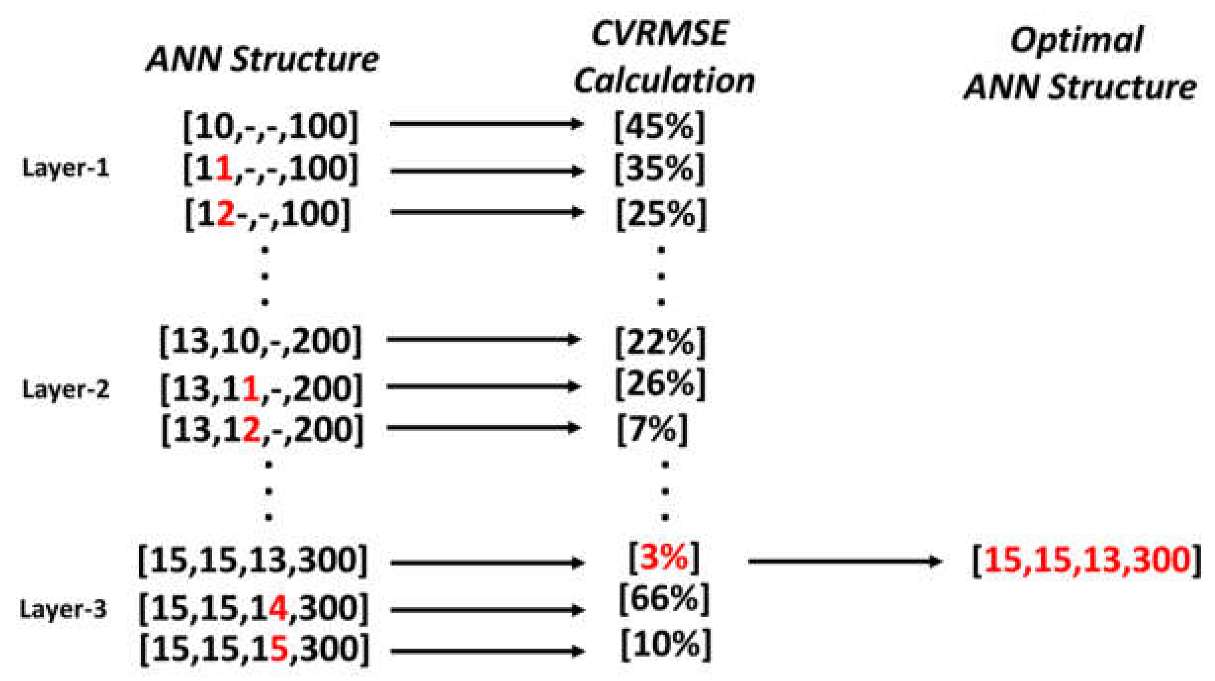
Figure 4 shows an example of the optimization of ANN structure. The optimization process involved evaluating the prediction accuracy of various conditions, ranging from 1 hidden layer, ten hidden nodes, and 100 epochs to 3 hidden layers, 15 hidden nodes, and 300 epochs for each algorithm. In total, 774 conditions were compared to identify the optimal structure for predicting the cooling load.

3. Simulation Study

3.1. Simulation Program

This study used the EnergyPlus simulation program developed by the U.S. Department of Energy (U.S. DOE) to ensure detailed analysis. The EnergyPlus program is a simulation program that combines the advantages of BLAST and DOE-2 and uses the heat balance method recommended by the American Society of Heating, Refrigerating, and Air-Conditioning Engineers (ASHRAE).
For the reliability verification of the EnergyPlus simulation program, simulation tools were developed and verified using ASHRAE Standard 140-2014 [29]. Eighty scenarios were tested and verified in three categories: building air-conditioning load, heating equipment, and cooling equipment. In addition, the EnergyPlus program was further reviewed using the IEA’s Building Energy Simulation Test.
In the EnergyPlus program, zone simulation analysis based on the integrated thermal and material equilibrium—the biggest drawback of the DOE-2 program—is possible. In addition, the analysis of flow between multiple zones, the analysis of pollutants generated in buildings, and the analysis of renewable energy systems are supported.

3.2. Target Building and Simulation Model

The Target building in this study is an office built in 2014 in the Research Triangle Park (RTP) area, NC, USA. The three-story structure includes offices, conference rooms, common areas, and storage spaces. The floor area is 4310 m2 ,   and the window-to-wall ratio is 23.3%. The HVAC system operates from 7 a.m. to 8 p.m. Figure 5 shows an overview of Target Building A.
The simulation model was developed using EnergyPlus version 9.4. Simulation conditions were mostly taken from real building values. Table 3 shows the people density in each space type in the target building. For example, lighting power density is 8.07 W/m2, while equipment power density is 10.76 W/m2. Table 4 provides details on the construction and material properties of the simulation model, which are all based on the target building.
Three AHUs are installed as the target building’s main heating and cooling system. A district heating and cooling system supplies chilled water and hot water to the AHUs for space cooling and heating. The AHUs provide cold or hot air to conditioned zones through the variable air volume fan. The cooling setpoint of the target building is 22.2 °C during office hours between 7 a.m. and 8 p.m. At night, the setback setpoint is 26.6 °C. We also used a throttling range of 1.1 °C for the cooling setpoint. The AHUs discharge air temperature (DAT) is 12.8 °C. For the detailed analysis, we selected the AHU installed on the second floor for the space heating and cooling.
In our research, we utilized a district cooling system. We used Equations (14) and (15) to convert the usage for chilled water ( C H W ) into the corresponding electricity consumption of the district cooling system. The estimation was based on assuming a Coefficient of Performance ( C O P ) value of 5, equivalent to 0.7 kW/ton [30]. This C O P value represents the recommended minimum requirement for Chiller C O P , as suggested by the NC Department of Environmental Quality in their Energy Saving Fact Sheet: Chillers report [30].
C H W e l e c t r i c i t y = T O R C O P c h i l l e r , a v g
where
C H W e l e c t r i c i t y = chilled water electricity consumption (kWh)
T O R = A ton of refrigeration (ton-hour); 1 TOR = 3.5169 kWh
C O P c h i l l e r , a v g   = typical C O P value of chiller (0.7 kW/ton)
T O R = C H W u s s e d C F
where
T O R = A ton of refrigeration (ton-hour); 1 TOR = 3.5169 kWh
C H W u s e d = chilled water usage (MJ)
C F = MJ to T O R conversion factor; 0.07898476 ton-hour/MJ

3.3. Calibration Process

In the measurement & verification (M&V) standard, the accuracy of the simulation model is assessed by comparing simulation results with actual experimental data. The ASHRAE Guideline 14-2014 [29], the International Performance Measurement and Verification Protocol [31], and the Federal Energy Management Program are representative M&V guides [32] and are indicators for the accuracy of simulation models.
The allowable error rate of the tolerance range varies depending on which of the three M&V guides is used. When we performed a correction with monthly data, the allowable tolerance range differed for each guide. However, when we calibrated the simulation model with hourly data, the tolerance range for all three M&V guides was the same at ±10% for normalized mean bias error (NMBE) and 30% for c v R M S E [29,31,32].
In this study, the simulation model was calibrated with hourly data, and the tolerance range was based on NMBE ± 10% and c v R M S E 30%. We used Equations (16) to (18) to calculate NMBE and c v R M S E .
R M S E = S M i n t e r v a l 2 N i n t e r v a l
c v R M S E = R M S E p e r i o d A p e r i o d
A p e r i o d = p e r i o d M i n t e r v a l N i n t e r v a l
where
S = ANN model prediction value,
M = EnergyPlus simulation results,
N i n t e r v a l = number of EnergyPlus results, and
A p e r i o d = measurement period average.
The data collection period for the target building A was from 10 May 2017 to 7 August 2017. Except for periods when there was a system problem, or the system was turned off, all data were normally collected from 4 July 2017 to 7 August 2017. During the periods when data were collected, the simulation model was calibrated, particularly during the hottest week of 17–21 July 2017, as this study aims to propose a control to save cooling energy.
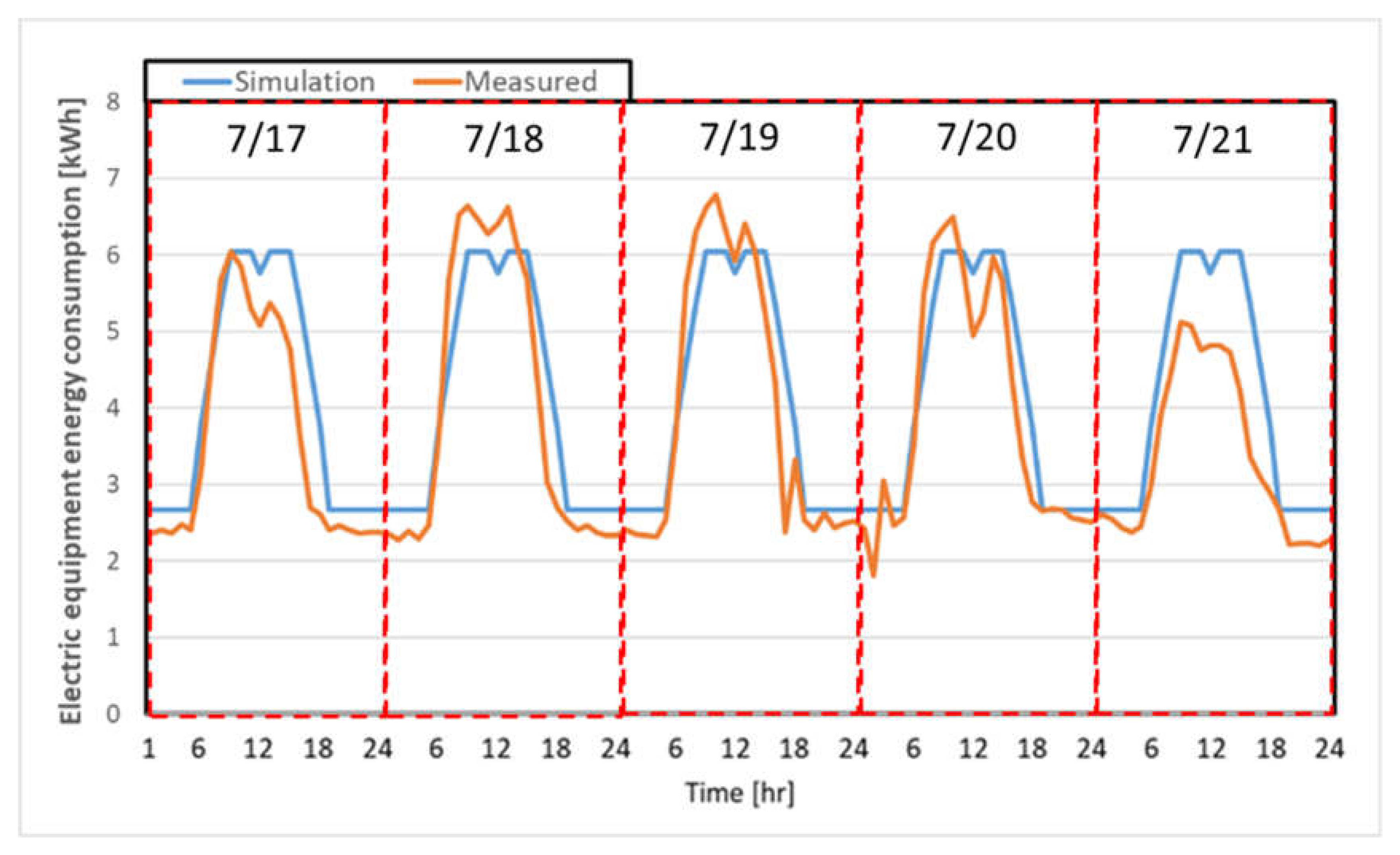
Figure 6, Figure 7 and Figure 8 show the comparison of field data and simulation results for lighting electricity energy consumption, electric equipment electricity energy consumption, and electrical energy consumption for heating and cooling during the selected week. For lighting electricity energy consumption, NMBE was 1.15%, whereas c v R M S E was 23%. For electric equipment electricity energy consumption, NMBE was 8.96%, whereas c v R M S E was 18.9%. Finally, regarding electricity energy consumption for heating and cooling, NMBE was 1.13%, whereas c v R M S E was 21.3%. Since both NMBE and c v R M S E were within the tolerance range described above, the simulation model was considered calibrated.

4. Case Study

4.1. Simulation Cases

This study had three simulation cases. In Case 1, the base case, the AHU-DAT was fixed at the actual control value of 12.8 °C for the target building. In Case 2, an optimized ANN-based cooling load prediction model was used to predict and control the AHU-DAT within the range of 12.8 °C to 17.8 °C based on the partial load section. Meanwhile, in Case 3, an optimized LSTM-based cooling load prediction model was used to predict and control the AHU-DAT within the same range. Finally, we compared the cooling electricity consumption on a representative day in a case study for each of the three cases. We evaluated the energy-saving ability of ML-based AHU-DAT control.

4.2. ML-Based HVAC Control Methods

Figure 9 and Table 5 present the AHU-DAT determination method for Cases 1, 2, and 3 based on the part load ratio (PLR) change in this study. In Case 1, the AHU-DAT was fixed at 12.8 °C, the actual AHU-DAT setpoint temperature in the test building. In Cases 2 and 3, the AHU-DAT setpoint temperatures were set within the 12.8 to 17.8 °C range based on the PLR interval predicted by the ANN and LSTM models. We conducted a simulation analysis and selected the temperature range of 12.8 to 17.8 °C, which falls within the allowable range of ±1.1 °C for the indoor cooling set temperature of 22.2 °C during office hours and 26.6 °C during the night. Notably, in Case 1, AHU-DAT was fixed at 12.8 °C regardless of changes in cooling load. In contrast, in Cases 2 and 3, AHU-DAT was controlled at 12.8 °C when the cooling load was predicted to be in the PLR 90–100% range and at 17.8 °C when the cooling load was predicted to be in the PLR 0–10% range to adapt the AHU-DAT control according to the change in cooling load.

5. Analysis and Results

5.1. Weather Conditions

Figure 10 presents the outdoor air temperature pattern in Raleigh, North Carolina, where the target building is located. The Raleigh weather file provided by EnergyPlus was modified using actual outdoor air temperature and humidity data collected from the target building in 2017 and total solar radiation collected from Raleigh Durham Airport. The outdoor air dry-bulb temperature range during the analysis period is 13.1–37.4 °C, and the outdoor air relative humidity during the analysis period is 20–100%.

5.2. Evaluation of Cooling Load Prediction Model Accuracy

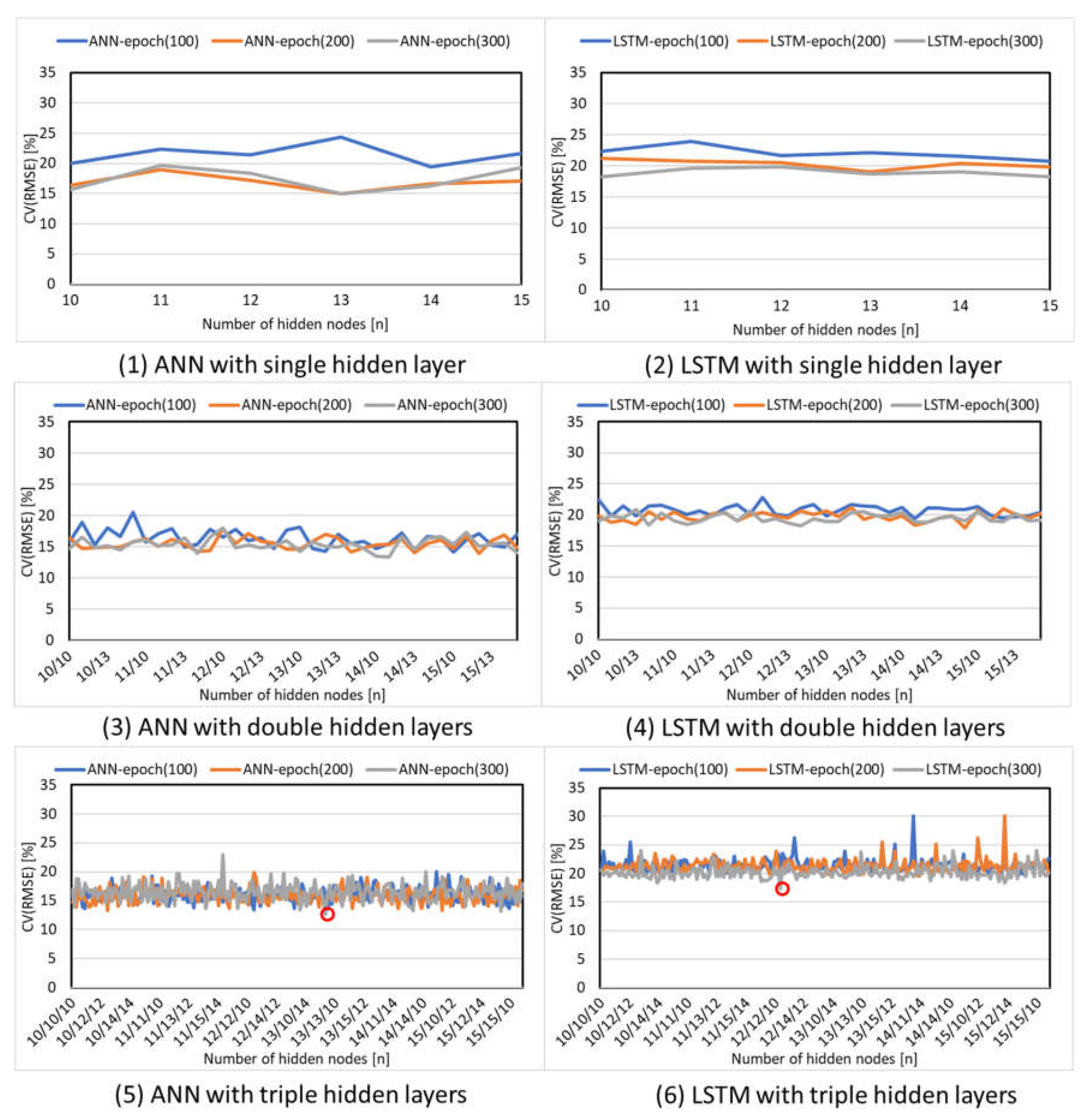
In this study, the hyperparameters (i.e., number of hidden layers, hidden nodes, and epochs) were selected and optimized for ANN and LSTM algorithms to enhance their performance. Figure 11 shows the cooling load prediction accuracy based on the different configurations of hidden nodes, epochs, and several hidden layers in the ANN and LSTM models. We observed that both algorithms achieved the highest prediction accuracy using hidden triple layers and 300 epochs.
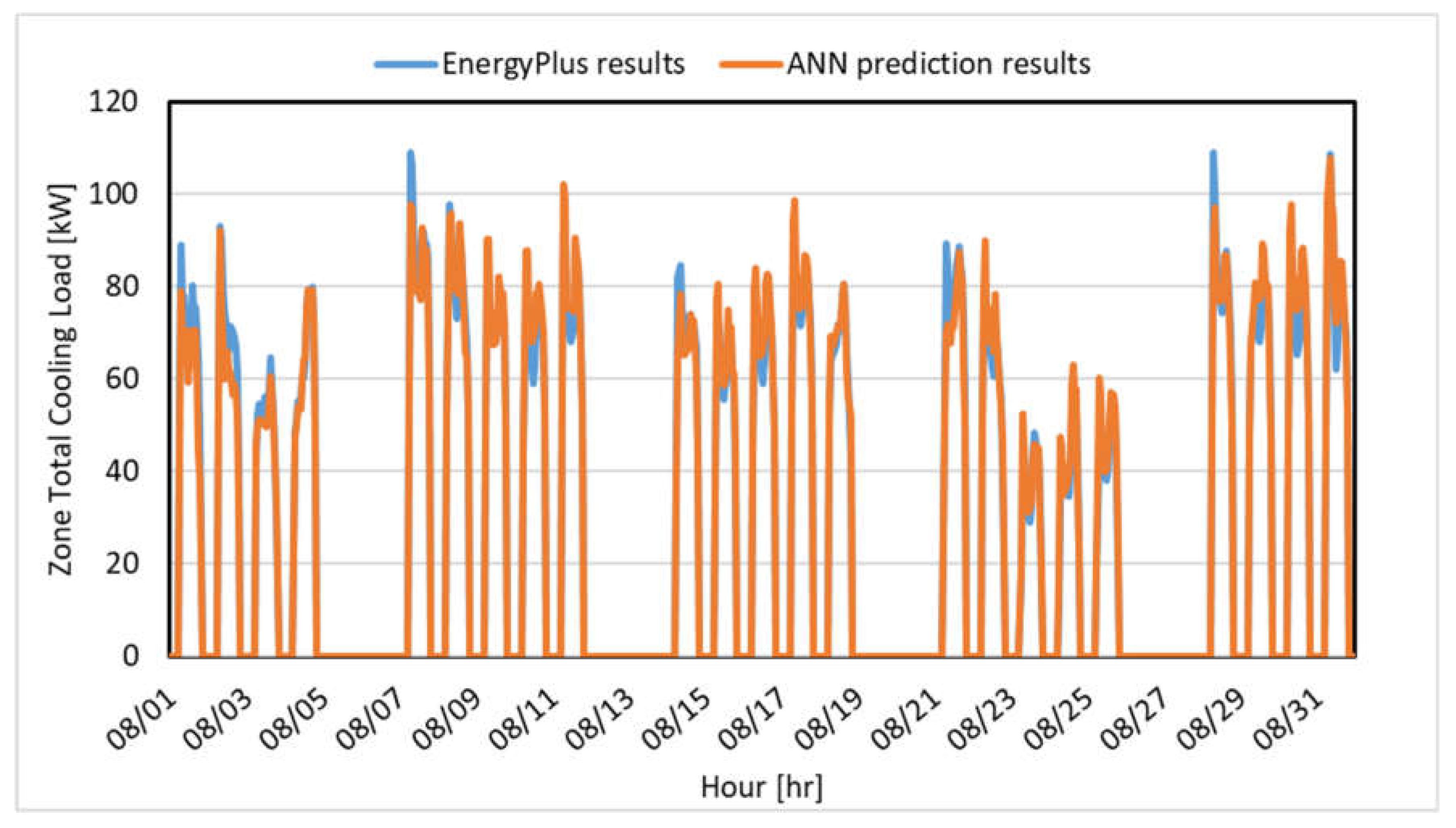
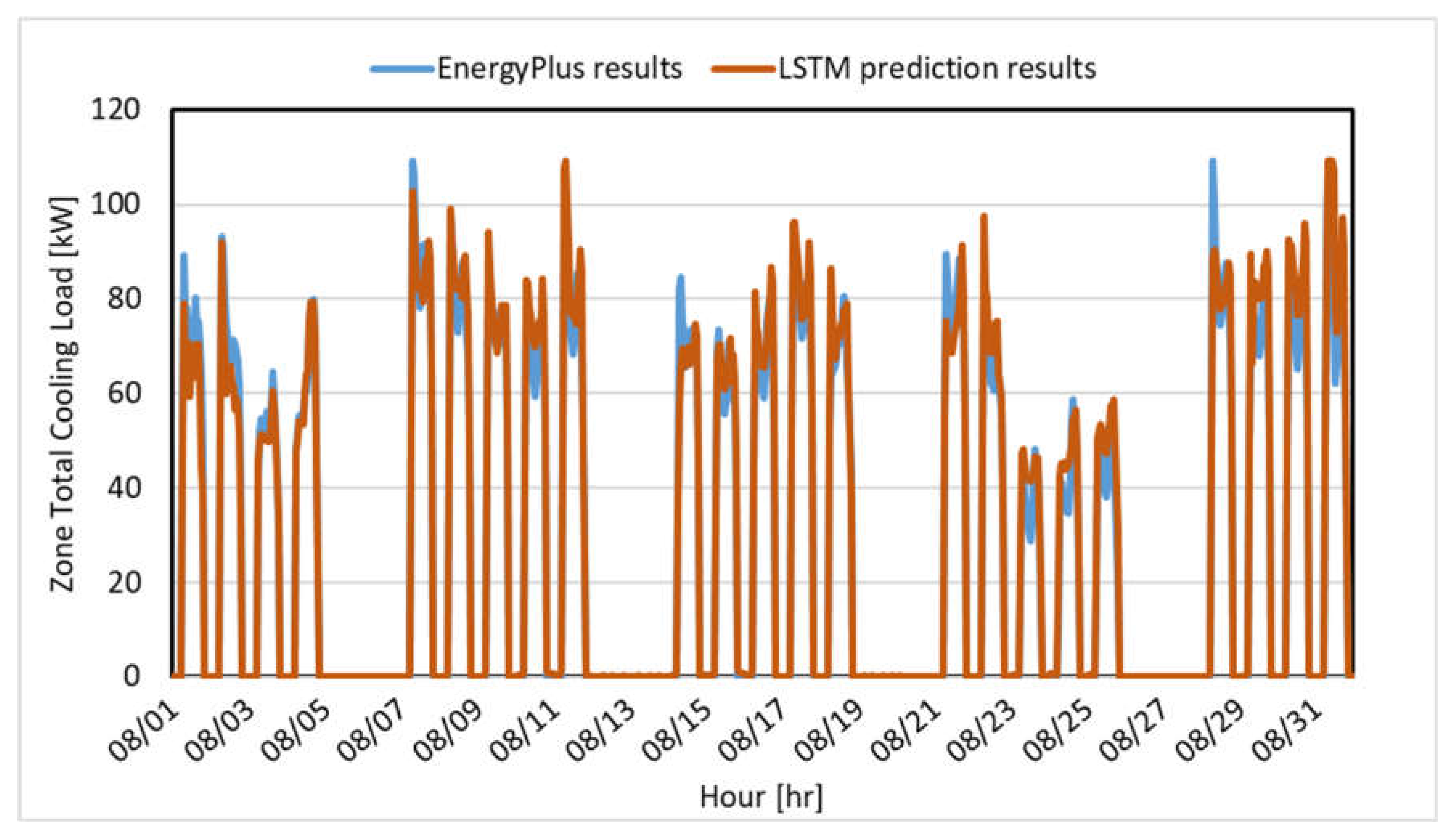
The optimized algorithm structures and their corresponding prediction accuracy are presented in Table 6. The prediction accuracy, as indicated by CV(RMSE), was 12.7% for ANN and 17.3% for LSTM, demonstrating a certain level of reliability for both optimized algorithms. However, the ANN algorithm has a higher prediction accuracy than the LSTM algorithm. This result can be attributed to the differences in the characteristics of the two algorithms. For example, LSTM incorporates past output data into the current input data, allowing for time-dependent learning. On the other hand, ANN treats all input data independently without considering the time sequence [3,4,5,6,7,8,9,10,11,12]. Due to these algorithm differences, LSTM is relatively more sensitive to patterns in past data than ANN [14,15,16,17,18,19,23,25].
Figure 12 depicts the pattern of outdoor air temperature, which directly impacts the cooling load of the building, among the input data used for training the ANN and LSTM models during June and July 2017. Examining the figure, we observed that the outside air temperature exhibits rapid fluctuations in three sections.
A comparison of the average outdoor air temperature during the building’s office hours from 7 AM to 8 PM revealed the following trends: In the first section, the average outdoor air temperature on 11 June was 26.5 °C, which decreased to 22.5 °C on 12 June and subsequently rose to 28.1 °C on 13 June. In the second section, the average outdoor air temperature on 25 June was 29.7 °C, followed by a decrease to 23.5 °C on 26 June and then a rise to 28.1 °C on 27 June. Meanwhile, in the third section, the average outdoor air temperature was 31.4 °C on 6 July but decreased to 24.9 °C on 7 July. Considering the rapid changes in the data trends that impact the cooling load, we inferred that the learning rate of the LSTM model shows a relatively lower prediction accuracy than that of the ANN model.
Figure 13 and Figure 14 compare the predicted cooling load generated by the optimized ANN and LSTM algorithms and the actual cooling load obtained from simulations from 1 August to 31 August.

5.3. AHU-DAT Operating Scenarios Comparison

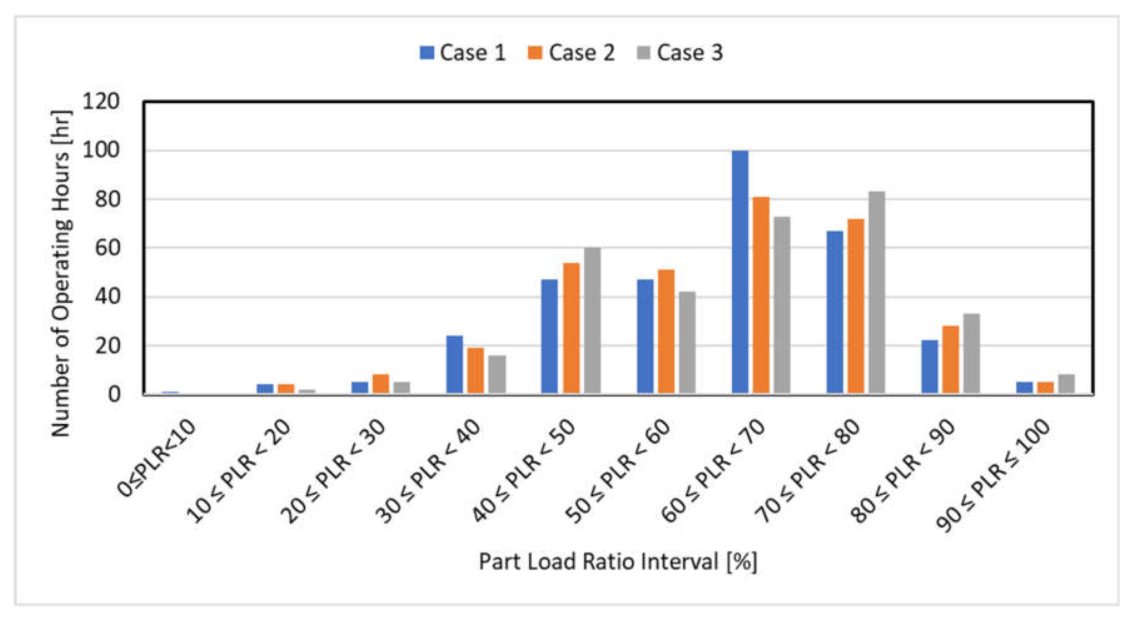
Figure 15 and Table 7 present the AHU-DAT operating scenarios for the three cases. We examined the impact of cooling load prediction accuracy on HVAC control by comparing the patterns of AHU-DAT control values. For each case, we constructed the scenarios based on the simulation results for Case 1 and the predicted cooling load for Cases 2 and 3. Additionally, we developed AHU-DAT scenarios for different PLR intervals, as shown in Table 5. The analysis focused on office hours in August.
According to Figure 15 and Table 7, when examining the load pattern of Case 1, a considerable amount of time (i.e., 241 h or 74.8% of the total hours) belonged to the PLR 50% above section. Within this section, the PLR range of 60% to less than 70% accounted for the highest duration, with 100 h. The next highest duration was observed in the PLR range of 70% to less than 80%, totaling 67 h.
In the load pattern of Case 2, a substantial duration of time (i.e., 237 h or 73.6% of the total hours) belonged to the PLR 50% above section. Within this section, the PLR range of 60% to less than 70% accounted for the highest duration, with 81 h. The next highest duration was observed in the PLR range of 70% to less than 80%, totaling 72 h.
In the load pattern of Case 3, a significant portion of the time (i.e., 239 h or 74.2% of the total hours) belonged to the PLR 50% above section. Notably, the PLR range of 60% to less than 70% had the highest duration, with 73 h. The next highest duration was observed in the PLR range of 70% to less than 80%, totaling 83 h.
Comparing the cumulative hours of PLR ranges among the cases, for the PLR range of 60% to less than 70%, Case 2 showed 19% fewer cumulative hours than Case 1. Case 3 exhibited 27% fewer cumulative hours compared to Case 1. Additionally, for the PLR range of 70% to less than 80%, Case 2 showed 7% more cumulative hours than Case 1. In contrast, Case 3 demonstrated 24% more cumulative hours than Case 1. Based on the analysis of the AHU-DAT operating scenarios for the three cases and the evaluation of prediction accuracy conducted in Section 5.2, it has been concluded that the ANN algorithm exhibits superior performance in predicting the load pattern of the target building compared to the LSTM algorithm. Considering the prediction accuracies of both models, it can be determined that the ANN algorithm is the more appropriate choice for controlling the HVAC system of the target building.

5.4. Weather Conditions on the Representative Day

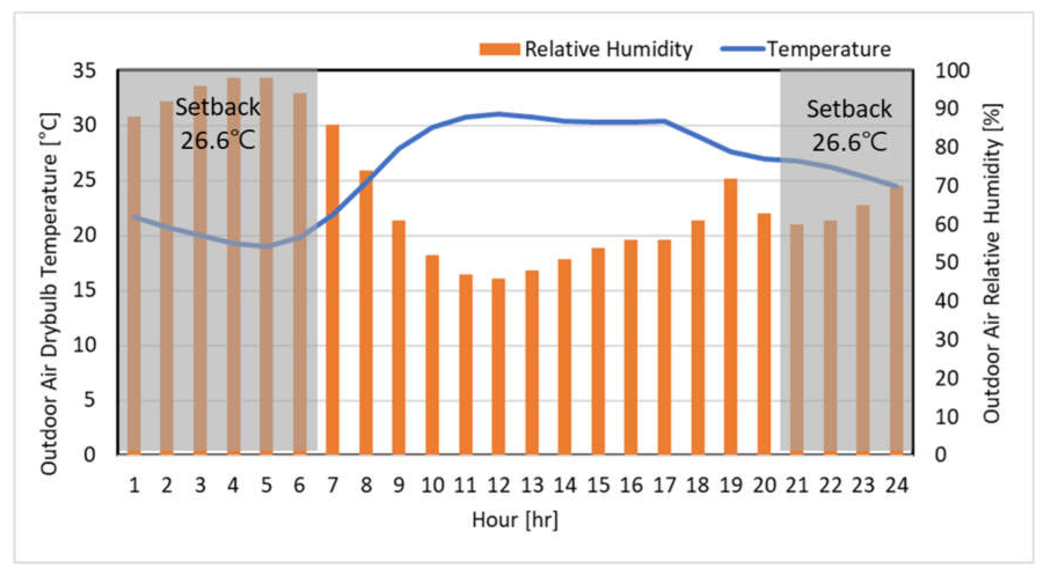
In this study, we conducted a feasibility analysis by analyzing a representative day to evaluate the potential of ML-based HVAC control in the target building. The test period for the ANN and LSTM algorithms was the month of August. Regarding the hottest day, it was difficult to compare the difference in control values by case because the PLR continued to maintain more than 80% most of the time. Therefore, we selected August 15, the median value of the outdoor air temperature, as the representative summer day. Figure 16 shows the outdoor air temperature and humidity variations on the summer representative day. The lowest outdoor air temperature was 19.0 °C, while the highest was 31.0 °C. The lowest outdoor air relative humidity was 46%, whereas the highest outdoor air relative humidity was 98%. Analyzing the characteristics of office hours between 7 a.m. and 8 p.m., we observed that the outdoor air temperature was at its lowest at 22 °C, while the outdoor air humidity was at its highest at 86% at 7 a.m. The outdoor air temperature peaked at 31 °C, while the outdoor air humidity reached its lowest point of 46% at noon.

5.5. Sensitivity Analysis of Zone Mean Air Temperature According to AHU-DAT Change on the Representative Day

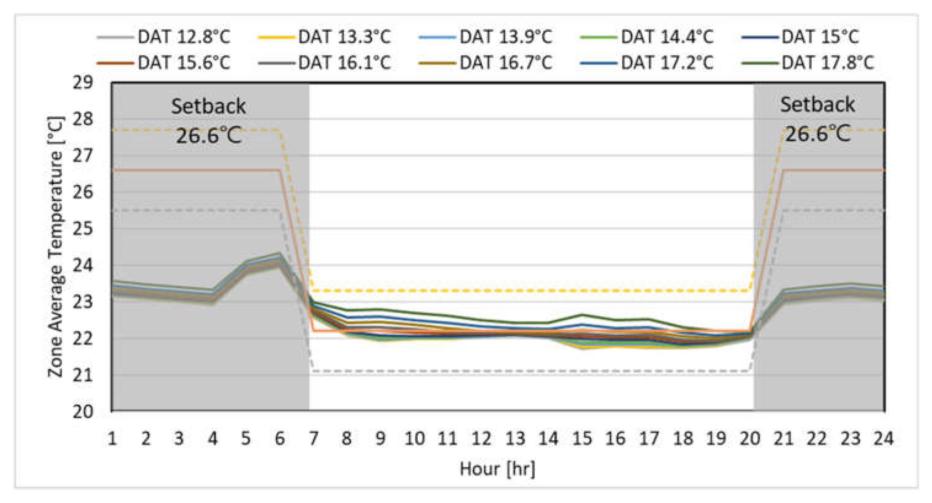
Figure 17 illustrates the variation in the average indoor air temperature across all zones connected to the AHU. DAT in the figure means AHU-DAT. The results indicate that the indoor air temperature on a representative day consistently meets the cooling set temperature of 22.2 °C, with a throttling range of 1.1 °C during office hours, regardless of AHU-DAT conditions. Furthermore, during the night, the indoor air temperature does not rise above the designated setback temperature of 26.6 °C, which means there is no need for the cooling system to activate. For this reason, the set temperature range specified for AHU-DAT control in Cases 2 and 3 is deemed suitable for maintaining the indoor cooling set temperature. AHU-DAT control was based on the predicted cooling partial load on a representative day, utilizing ANN and LSTM algorithms with AHU-DAT set in 10 selected temperature ranges.

5.6. Comparison of AHU-DAT Pattern on the Representative Day

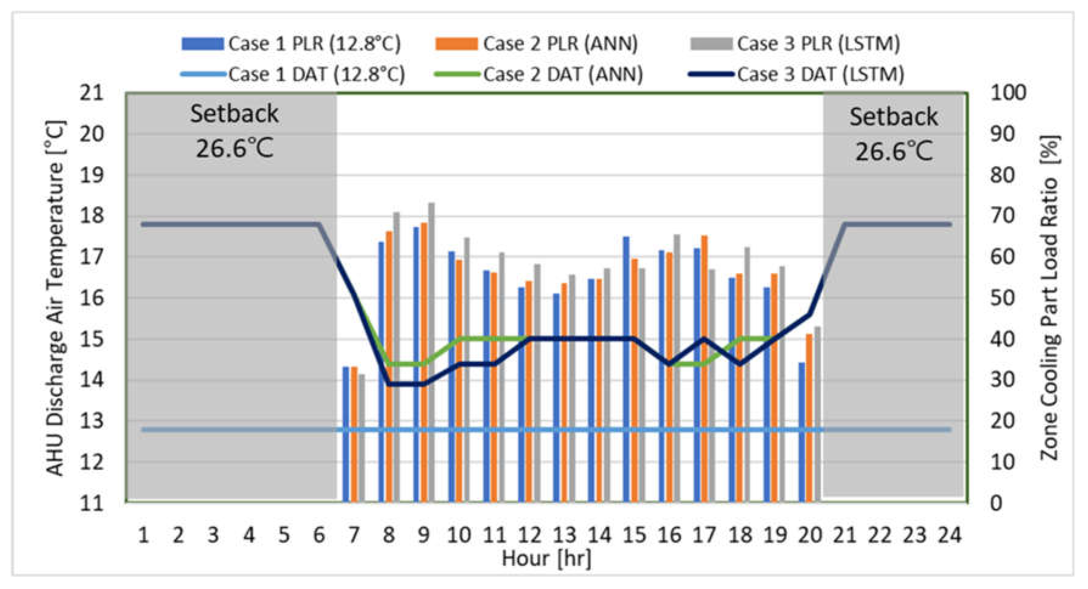
Figure 18 depicts the variation in AHU-DAT based on the PLR on the summer representative day, analyzed by case. The PLR pattern on a representative day increases sharply from 8 a.m. across all cases, decreases around noon, and follows a pattern similar to the change in outdoor air temperature until 8 p.m. This pattern is attributed to the rapid fluctuation in outdoor air temperature from 22 °C at 7 a.m. to 25 °C at 8 a.m. and the consideration of internal heat gain schedules, accounting for reduced building utilization during lunchtime.
When comparing the PLR in each case, Case 1 served as the base case. It reflected the PLR obtained by dividing the cooling load for each hour, calculated through the EnergyPlus simulation model, by the maximum cooling load during summer. Conversely, in Cases 2 and 3, as explained in Section 3.1, the algorithms learned the cooling load pattern according to the input variables during the learning period, and based on this, they predicted the cooling load on a representative day.
In Cases 2 and 3, the predicted cooling load was divided by the same maximum cooling load value as in Case 1 to determine the PLR for control purposes. Although the same input variables were employed, the predicted cooling PLR in Cases 2 and 3 tended to differ due to variations in prediction accuracy arising from the characteristics of the algorithm.
An examination of the AHU-DAT set values for each case revealed that Case 1 maintained a constant temperature of 12.8 °C irrespective of changes in the PLR. In contrast, Cases 2 and 3 exhibited distinct AHU-DAT values corresponding to the predicted PLR. For example, in Case 2, AHU-DAT was controlled at 16.0 °C at 7 a.m.. As a result, the lowest predicted PLR, and at 14.4 °C around 9 a.m., the highest predicted PLR. Meanwhile, in Case 3, AHU-DAT was controlled at 16.0 °C at 7 a.m., the lowest predicted PLR, and at 13.9 °C around 9 a.m., the highest predicted PLR.
This discrepancy is attributed to the variation in AHU-DAT control values for each 10% interval of the PLR, as illustrated in Figure 9 and Table 5. The predicted PLR at 9 a.m. for Case 2 falls within 60% or more and less than 70%, specifically at 68.4%. Meanwhile, the predicted PLR for Case 3 is 70.9%, which falls within 70% or more and less than 80%. Although the predicted PLR at 9 a.m. for Case 1 is 67.3%, which is not significantly different from that in Cases 2 and 3, differences in AHU-DAT occur as the PLR section changes. However, it was determined that the 4.6% difference in Cases 2 and 3 prediction accuracy was not significant enough to change control of the AHU-DAT at each hour. In this study, AHU-DAT control was performed by dividing the intervals by PLR at 10% intervals (see Figure 8). Accordingly, we reckoned that there was a limit to control AHU-DAT by sufficiently reflecting the 4.6% difference in prediction accuracy between Case 2 and Case 3.
During the night, the AHU-DAT of Case 2 and 3 was controlled at 17.8 °C because no cooling load was required due to the indoor air temperature not rising above the set temperature of 26.6 °C, as shown in Figure 18.
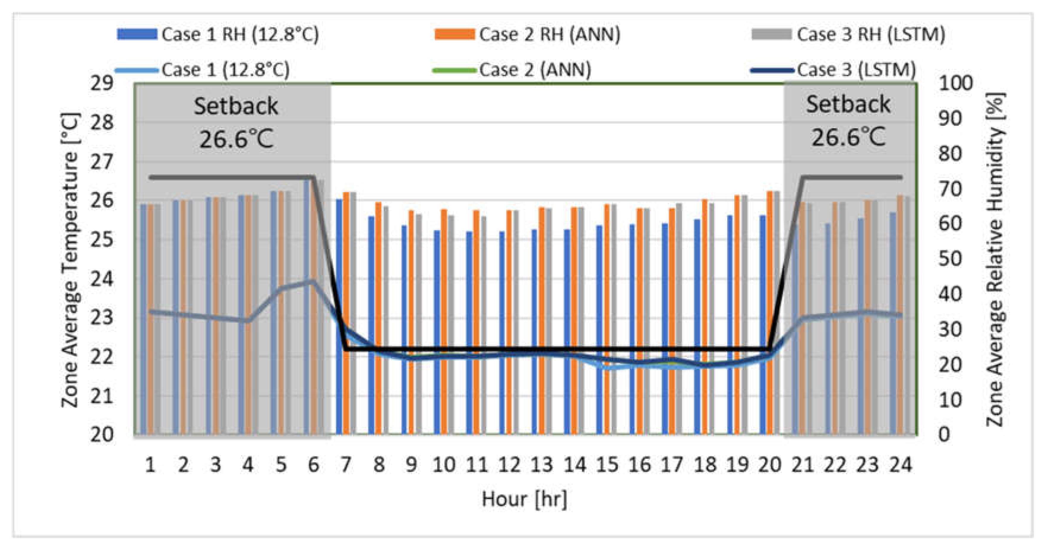
Figure 19 compares averaged indoor air temperature and relative humidity for each case. It can be observed that all cases met the tolerance of 22.2 ± 1.1 °C for indoor air temperature. Additionally, the indoor relative humidity remained below 70% in all sections. Notably, Cases 2 and 3 exhibited a higher indoor air temperature of 22.2 °C compared to Case 1, as AHU-DAT was controlled at a higher set temperature in these cases.

5.7. Comparison of Total Cooling Energy Consumption on the Representative Day

Figure 20 and Table 8 show the total cooling electricity consumption, including CHW used (MJ/day), TOR (ton-hour/day), CHW electricity consumption (kWh/day), CHW pump electricity consumption (kWh/day), and fan electricity consumption (kWh/day) in each case on the summer representative day. For example, case 1 showed CHW using about 3060.0 MJ/day, while Case 2 showed about 2870.2 MJ/day and 2875.7 MJ/day on the summer representative day. Also, Case 1 consumed a TOR of 241.7 ton-hour/day, whereas Cases 2 and 3 consumed about 226.7 ton-hour/day and 227.1 ton-hour/day, respectively.
Regarding CHW electricity consumption, Case 1 consumed 169.2 kWh/day, while Case 2 and Case 3 consumed 158.7 kWh/day and 159.0 kWh/day, respectively. Comparing the CHW energy consumption of Cases 1 and 2, Case 2 saved 6.2% more CHW energy than Case 1. Meanwhile, Case 3 saved 6.0% more CHW energy than Case 1.
On the summer representative day, Case 1 consumed about 12.3 kWh/day for CHW pump electricity, while Case 2 and Case 3 consumed about 10.7 kWh/day and 10.8 kWh/day, respectively. Comparing the CHW pump electricity consumption of Cases 1 and 2, Case 2 consumed 12.5% less than Case 1. Meanwhile, comparing the CHW pump electricity consumption of Cases 1 and 3, Case 3 consumed 11.8% less than Case 1. Controlling the AHU-DAT through the ANN and LSTM algorithms significantly reduced CHW electricity consumption and CHW pump consumption compared to that of a fixed AHU-DAT.
Regarding the supply fan, the fan electricity consumption of Case 1 on the summer representative day was about 10.8 kWh/day, while Case 2 and Case 3 consumed about 16.7 kWh/day and about 16.1 kWh/day, respectively. Comparing the fan electricity consumption of Cases 1 and 2, Case 2 consumed 55.2% more than Case 1. Meanwhile, comparing Cases 1 and 3, Case 3 consumed 49.4% more fan electricity than Case 1.
In Case 1, fan air volume was decreased when the required cooling load was reduced, whereas in Cases 2 and 3, the AHU-DAT was increased in response to the lowered cooling load, resulting in increased fan air volume and decreased CHW flow rate. As a result of this difference, Cases 2 and 3 exhibited lower energy consumption for both CHW and pump but higher fan consumption compared to Case 1. Regarding the combined electricity consumption for CHW, pump, and fan, Case 2 achieved cooling energy savings of 3.2%, while Case 3 showed cooling energy savings of 3.3% compared to Case 1. Through these results, we determined that ML-based AHU-DAT control has the potential to save energy compared to fixed AHU-DAT control.

6. Conclusions

In this study, we aimed to compare the accuracy of cooling load prediction using ANN and LSTM algorithms, widely utilized in building energy research, to determine the optimal algorithm for controlling HVAC systems in the target building.
Based on the comparison of CV(RMSE) values, the ANN algorithm demonstrated higher prediction accuracy than LSTM, with a CV(RMSE) value of 12.7% for ANN and 17.3% for LSTM. We analyzed that the rapid changes in historical data trends of the target building made LSTM relatively less effective. This is because ANN treats all input data independently, while LSTM processes input and output data in its internal memory to relate all input and output values. Furthermore, by analyzing the AHU-DAT operating scenarios for the three cases, we determined that the ANN algorithm exhibits superior performance in predicting the load pattern of the target building compared to the LSTM algorithm. Taking into consideration the prediction accuracies and the AHU-DAT operating scenarios of both models, we concluded that the ANN algorithm is the more suitable choice for controlling the HVAC system in the target building.
Three cases were considered to assess the cooling energy consumption of ML-based HVAC control methods: Case 1 with a fixed AHU-DAT control at 12.8 °C, Case 2 with an ANN-based predictive control, and Case 3 with an LSTM-based predictive control. In addition, this study considered the control strategy of adjusting the AHU-DAT for each 10% interval of the PLR based on the cooling load predictions from Case 2 and Case 3. The results indicated that Case 2 can save cooling energy consumption by 3.2%, while Case 3 can save 3.3% consumption compared to Case 1. Therefore, it was determined that ML-based AHU-DAT control could save energy compared to fixed AHU-DAT control.
However, according to the AHU-DAT pattern of the representative day, the 4.6% difference in Cases 2 and 3 prediction accuracy was not significant enough to change control of the AHU-DAT at each PLR 10% interval. To address this issue in the future, we intend to research predictive control of Air Handling Unit-Discharge Air Temperature (AHU-DAT) by dividing Part Load Ratio (PLR) sections based on the load characteristics of the target building in various scenarios. Instead of dividing sections into 10% intervals, this approach will ensure more precise control. We also plan to conduct a comparative analysis of Fuzzy logic-based HVAC control and ML-based HVAC control methods. Additionally, we will evaluate the energy efficiency of ML-based HVAC control methods by selecting low, medium, and high load days and performing a comparative analysis monthly.

Author Contributions

Conceptualization, B.S.; Methodology, B.S., Y.Y. and S.C.; Software, B.S. and Y.Y.; Formal analysis, B.S. and Y.Y.; Investigation, B.S., K.H.L. and S.C.; Writing—original draft, Y.Y., B.S. and K.H.L.; Writing—review & editing, Y.Y., B.S., K.H.L. and S.C.; Visualization, B.S. and Y.Y.; Supervision, S.C. All authors have read and agreed to the published version of the manuscript.

Funding

This research was funded by the Technology Innovation Program (or Industrial Strategic Technology Development Program, 20014154, Development of EMS with Optimal Control Algorithm for Energy Efficiency Improvement in Commercial Building Using AI and Digital Twin Technology) funded By the Ministry of Trade, Industry & Energy (MOTIE, Republic of Korea).

Informed Consent Statement

Not applicable.

Data Availability Statement

Data will be made available on request.

Conflicts of Interest

The authors declare no conflict of interest.

References

  1. U.S Energy Information Administration (EIA). Annual Energy Outlook 2019. 2019. Available online: https://www.eia.gov/todayinenergy/detail.php?id=38112 (accessed on 17 April 2023).
  2. International Energy Agency (IEA). The Future of Cooling. 2018. Available online: https://www.iea.org/reports/the-future-of-cooling (accessed on 17 April 2023).
  3. Yeon, S.; Yu, B.; Seo, B.; Yoon, Y.; Lee, K.H. ANN based automatic slat angle control of venetian blind for minimized total load in an office building. Sol. Energy 2019, 180, 133–145. [Google Scholar] [CrossRef]
  4. Seo, B.M.; Yoon, Y.B.; Song, S.; Cho, S. ANN-based thermal load prediction approach for advanced controls in building energy systems. In Proceedings of the Conference for ARCC 2019 International Conference, Toronto, ON, Canada, 29 May–1 June 2019. [Google Scholar]
  5. Lee, J.M.; Hong, S.H.; Seo, B.M.; Lee, K.H. Application of artificial neural networks for optimized AHU discharge air temperature set-point and minimized cooling energy in VAV system. Appl. Therm. Eng. 2019, 153, 726–738. [Google Scholar] [CrossRef]
  6. Qian, F.; Gao, W.; Yang, Y.; Yu, D. Potential analysis of the transfer learning model in short and medium-term forecasting of building HVAC energy consumption. Energy 2020, 193, 116724. [Google Scholar] [CrossRef]
  7. Moon, J.W.; Yang, Y.K.; Choi, E.J.; Choi, Y.J.; Lee, K.-H.; Kim, Y.-S.; Park, B.R. Development of a control algorithm aiming at cost-effective operation of a VRF heating system. Appl. Therm. Eng. 2019, 149, 1522–1531. [Google Scholar] [CrossRef]
  8. Park, B.R.; Choi, E.J.; Hong, J.; Lee, J.H.; Moon, J.W. Development of an energy cost prediction model for a VRF heating system. Appl. Therm. Eng. 2018, 140, 476–486. [Google Scholar] [CrossRef]
  9. Mtibaa, F.; Nguyen, K.-K.; Dermardiros, V.; Cheriet, M. Context-aware Model Predictive Control framework for multi-zone buildings. J. Build. Eng. 2021, 42, 102340. [Google Scholar] [CrossRef]
  10. Sendra-Arranz, R.; Gutiérrez, A. A long short-term memory artificial neural network to predict daily HVAC consumption in buildings. Energy Build. 2020, 216, 109952. [Google Scholar]
  11. Mba, L.; Meukam, P.; Kemajou, A. Application of artificial neural network for predicting hourly indoor air temperature and relative humidity in modern building in humid region. Energy Build. 2016, 121, 32–42. [Google Scholar] [CrossRef]
  12. Zhao, J.; Liu, X. A hybrid method of dynamic cooling and heating load forecasting for office buildings based on artificial intelligence and regression analysis. Energy Build. 2018, 174, 293–308. [Google Scholar] [CrossRef]
  13. Afram, A.; Janabi-Sharifi, F.; Fung, A.S.; Raahemifar, K. Artificial neural network (ANN) based model predictive control (MPC) and optimization of HVAC systems: A state of the art review and case study of a residential HVAC system. Energy Build. 2017, 141, 96–113. [Google Scholar] [CrossRef]
  14. Jang, J.; Han, J.; Leigh, S.-B. Prediction of heating energy consumption with operation pattern variables for non-residential buildings using LSTM networks. Energy Build. 2022, 255, 111647. [Google Scholar] [CrossRef]
  15. Faiq, M.; Tan, K.G.; Liew, C.P.; Hossain, F.; Tso, C.-P.; Lim, L.L.; Wong, A.Y.K.; Shah, Z.M. Prediction of energy consumption in campus buildings using long short-term memory. Alex. Eng. J. 2023, 67, 65–76. [Google Scholar] [CrossRef]
  16. Fang, Z.; Crimier, N.; Scanu, L.; Midelet, A.; Alyafi, A.; Delinchant, B. Multi-zone indoor temperature prediction with LSTM-based sequence to sequence model. Energy Build. 2021, 245, 111053. [Google Scholar] [CrossRef]
  17. Bouktif, S.; Fiaz, A.; Ouni, A.; Serhani, M.A. Optimal Deep Learning LSTM Model for Electric Load Forecasting using Feature Selection and Genetic Algorithm: Comparison with Machine Learning Approaches. Energies 2018, 11, 1636. [Google Scholar] [CrossRef]
  18. Somu, N.; Ramamritham, G.R.K. A deep learning framework for building energy consumption forecast. Renew. Sustain. Energy Rev. 2021, 137, 110591. [Google Scholar]
  19. Peng, C.; Tao, Y.; Chen, Z.; Zhang, Y.; Sun, X. Multi-source transfer learning guided ensemble LSTM for building multi-load forecasting. Expert Syst. Appl. 2022, 202, 117194. [Google Scholar] [CrossRef]
  20. Rashid, T. Make Your Own Neural Network; CreateSpace Independent Publishing Platform: North Charleston, SC, USA, 2016. [Google Scholar]
  21. Rumelhart, D.E.; Hinton, G.E.; Williams, R.J. Learning representations by back-propagating errors. Nature 1986, 323, 533–536. [Google Scholar] [CrossRef]
  22. Mittal, A. Understanding RNN and LSTM. 2019. Available online: https://towardsdatascience.com/understanding-rnn-and-lstm-f7cdf6dfc14e (accessed on 17 April 2023).
  23. Zarzycki, K.; Lawrynczuk, M. LSTM and GRU Neural Networks as Models of Dynamical Processes Used in Predictive Control: A Comparison of Models Developed for Two Chemical Reactors. Sensors 2021, 21, 5625. [Google Scholar] [CrossRef] [PubMed]
  24. Olah, C. Understanding LSTM Networks. 2015. Available online: https://colah.github.io/posts/2015-08-Understanding-LSTMs/ (accessed on 17 April 2023).
  25. Jung, M.; Mendes, P.R.d.C.; Önnheim, M.; Gustavsson, E. Model Predictive Control when utilizing LSTM as dynamic models. Eng. Appl. Artif. Intell. 2023, 123, 106226. [Google Scholar] [CrossRef]
  26. Keras. Available online: https://keras.io/about/ (accessed on 17 April 2023).
  27. Falk, R.F.; Miller, N.B. A Primer for Soft Modeling; University of Akron Press: Akron, OH, USA, 1992. [Google Scholar]
  28. Schober, P.; Boer, C.; Schwarte, L.A. Correlation Coefficients: Appropriate Use and Interpretation. Anesth Analg. 2018, 126, 1763–1768. [Google Scholar] [PubMed]
  29. ASHRAE. Guideline 14-2014. 2014. Measurement of Energy and Demand Savings; American Society of Heating, Refrigerating, and Air Conditioning Engineers: Atlanta, GA, USA, 2014. [Google Scholar]
  30. North Carolina Environmental Quality, Energy Saving Fact Sheet: Chillers. 2010. Available online: https://www.deq.nc.gov/environmental-assistance-and-customer-service/ias-energy-efficiency/opportunities/chillers/download (accessed on 26 April 2023).
  31. International Performance Measurement & Verification Protocol (IPMVP). Concepts and Options for Determining Energy and Water Savings. Volume 1, Section 3.4.4.2. 2002. Available online: https://www.nrel.gov/docs/fy02osti/31505.pdf (accessed on 26 April 2023).
  32. Federal Energy Management Program (FEMP). M&V Guidelines: Measurement and Verification for Performance-Based Contracts Version 4.0, Section 4.5.3. 2015. Available online: https://www.energy.gov/femp/articles/mv-guidelines-measurement-and-verification-performance-based-contracts-version-40 (accessed on 26 April 2023).
Figure 1. Overview of the research flow.
Buildings 13 01434 g001
Figure 2. ANN algorithm structure.
Buildings 13 01434 g002
Figure 3. LSTM algorithm structure.
Buildings 13 01434 g003
Figure 4. Example of the optimization process.
Buildings 13 01434 g004
Figure 5. Overview of Target Building A.
Buildings 13 01434 g005
Figure 6. Calibration results for lighting energy consumption.
Buildings 13 01434 g006
Figure 7. Calibration results for electric equipment energy consumption.
Buildings 13 01434 g007
Figure 8. Calibration results for HVAC system energy consumption.
Buildings 13 01434 g008
Figure 9. Comparison of AHU-DAT control values by PLR section in each case.
Buildings 13 01434 g009
Figure 10. Outdoor air dry-bulb temperature and relative humidity in Raleigh, North Carolina.
Buildings 13 01434 g010
Figure 11. Comparison of the predictive accuracy of the ANN and LSTM models according to hyperparameter changes.
Buildings 13 01434 g011
Figure 12. Outdoor air dry-bulb temperature and relative humidity in June and July in Raleigh, North Carolina.
Buildings 13 01434 g012
Figure 13. Comparison of simulation data and ANN results.
Buildings 13 01434 g013
Figure 14. Comparison of simulation data and LSTM result.
Buildings 13 01434 g014
Figure 15. AHU-DAT control scenarios during office hours in August.
Buildings 13 01434 g015
Figure 16. Outdoor air dry-bulb temperature and relative humidity pattern on a representative day.
Buildings 13 01434 g016
Figure 17. Sensitivity analysis of zone mean air temperature according to AHU-DAT change on a representative day.
Buildings 13 01434 g017
Figure 18. Comparison of the PLR and AHU-DAT pattern on a representative day.
Buildings 13 01434 g018
Figure 19. Comparison of the relative humidity and zone average temperature on a representative day.
Buildings 13 01434 g019
Figure 20. Comparison of the total cooling energy consumption on a representative day.
Buildings 13 01434 g020
Table 1. Correlation analysis results.
Correlation Factor with Cooling LoadOutdoor Air Temperature (°C)Outdoor Air Relative Humidity
(%)
Diffuse Solar Radiation
(W/m²)
Direct Solar Radiation
(W/m²)
Lighting Schedules
(%)
Electric Equipment Schedules
(%)
People Schedules
(%)
Day and Hour Type
(-)
r0.5621−0.50220.47370.48630.86940.83530.90610.9446
0.31590.25220.22430.23650.75580.69770.82100.8923
Table 2. Hyperparameters and ranges.
DivisionHyperparameter Range
ANNLSTM
Number of hidden layers [n]1, 2, 3
Number of hidden nodes [n]10~15
Epochs [n]100, 200, 300
Batch size [n]24
OptimizerAdam
Activation FunctionSigmoid and Rectified linear unit
Table 3. Target Building A’s people density in each space type.
Zone People   Density   ( m 2 / Person )
Break Room5.0
Closed Office12.1
Open Office12.1
Conference12.1
IT Room12.1
Lobby9.3
Corridor9.3
Mechanical Room14.0
Stair12.1
Rest Room14.9
Storage14.0
Table 4. Target Building A’s construction properties.
ConstructionU-Value
(W/m2 K)
Visible TransmittanceSolar Heat Gain Coefficient
Exterior Wall0.232XX
Interior Wall2.867XX
Roof0.174XX
Exterior window 1.650.600.31
Table 5. AHU-DAT control classes by PLR section in each case.
ClassAHU-DAT
(°C)
Case 1ClassAHU-DAT
(°C)
Cases 2 and 3
IntervalInterval
112.80% ≤ PLR < 10%117.8 0% ≤ PLR < 10%
212.810% ≤ PLR < 20%217.210% ≤ PLR < 20%
312.820% ≤ PLR < 30%316.720% ≤ PLR < 30%
412.830% ≤ PLR < 40%416.130% ≤ PLR < 40%
512.840% ≤ PLR < 50%515.640% ≤ PLR < 50%
612.850% ≤ PLR < 60%615.050% ≤ PLR < 60%
712.860% ≤ PLR < 70%714.460% ≤ PLR < 70%
812.870% ≤ PLR < 80%813.970% ≤ PLR < 80%
912.880% ≤ PLR < 90%913.380% ≤ PLR < 90%
1012.890% ≤ PLR ≤ 100%1012.890% ≤ PLR ≤ 100%
Table 6. Optimal structure and parameter values.
DivisionANNLSTM
Optimized ValuesOptimized Values
Number of Hidden Layers [n]33
Number of Hidden Neurons Layer 1 [n]1312
Number of Hidden Neurons Layer 2 [n]1212
Number of Hidden Neurons Layer 3 [n]1112
Epochs [n]300300
CV(RMSE) [%]12.717.3
Table 7. AHU-DAT operating scenarios during office hours in August.
ClassAHU-DAT
(°C)
Case 1AHU-DAT
(°C)
Case 2Case 3
IntervalNumber of Hours
(h)
IntervalNumber of Hours
(h)
IntervalNumber of Hours
(h)
112.80% ≤ PLR < 10%117.80% ≤ PLR < 10%-0% ≤ PLR < 10%-
212.810% ≤ PLR < 20%417.210% ≤ PLR < 20%410% ≤ PLR < 20%2
312.820% ≤ PLR < 30%516.720% ≤ PLR < 30%820% ≤ PLR < 30%5
412.830% ≤ PLR < 40%2416.130% ≤ PLR < 40%1930% ≤ PLR < 40%16
512.840% ≤ PLR < 50%4715.640% ≤ PLR < 50%5440% ≤ PLR < 50%60
612.850% ≤ PLR < 60%4715.050% ≤ PLR < 60%5150% ≤ PLR < 60%42
712.860% ≤ PLR < 70%10014.460% ≤ PLR < 70%8160% ≤ PLR < 70%73
812.870% ≤ PLR < 80%6713.970% ≤ PLR < 80%7270% ≤ PLR < 80%83
912.880% ≤ PLR < 90%2213.380% ≤ PLR < 90%2880% ≤ PLR < 90%33
1012.890% ≤ PLR ≤ 100%512.890% ≤ PLR ≤ 100%590% ≤ PLR ≤ 100%8
Total hours (h)322322322
Table 8. Comparison of the total cooling energy consumption on a representative day.
Case 1Case 2Case 3
CHW used (MJ/day)3060.02870.22875.7
TOR (ton-hour/day)241.7226.7227.1
CHW electricity consumption (kWh/day) based on COP 5 (0.7 kW/ton)169.2158.7159.0
CHW Pump electricity consumption (kWh/day)12.310.710.8
Fan electricity consumption (kWh/day)10.816.716.1
Total cooling electricity consumption (CHW+CHW pump+fan) [kWh/day]192.3186.1185.9
Disclaimer/Publisher’s Note: The statements, opinions and data contained in all publications are solely those of the individual author(s) and contributor(s) and not of MDPI and/or the editor(s). MDPI and/or the editor(s) disclaim responsibility for any injury to people or property resulting from any ideas, methods, instructions or products referred to in the content.