Article

Experience Grammar: Creative Space Planning with Generative Graph and Shape for Early Design Stage

School of Architecture, Design, and Planning, The University of Sydney, Sydney, NSW 2008, Australia
Buildings 2023, 13(4), 869; https://doi.org/10.3390/buildings13040869
Submission received: 27 February 2023 / Revised: 23 March 2023 / Accepted: 24 March 2023 / Published: 26 March 2023

Abstract

:
This paper presents a method to synthesise functional relationships and spatial configuration simultaneously using shape and graph computation from shape grammar and space syntax theories. The study revisits seminal works and summarises the compatibilities between shape and graph computation as a set of rules. The rule computation is demonstrated in two cases from hospitality and retail, where current applications, opportunities, and limitations are discussed. The results from the study show that incorporating graph and shape rules allows sequences of functions and spatial arrangements to be developed in parallel. The method could help the designer anticipate the impact on the users’ flow of activities more explicitly during the early design process and could also assist in generating new functional configurations to provide alternative spatial strategies in broader applications.

1. Introduction

Building occupancy modes have been rapidly shifting in the past decade as users adapt to trends in technology and global issues (e.g., the COVID-19 pandemic and IoT). As users reinvent their businesses, functional configuration in a building sometimes becomes contested, and design strategies relying on aesthetic and form articulation do not always provide satisfactory answers [1,2]. While form-centric design remains commonly practised, diverse logic on how a building adapts to functional changes—and how a function adjusts to a building—is becoming more necessary today. This includes the logic of how users transform the space to fit new functions or modify their functions to suit existing spaces. A new-looking building might be operating for a conventional function, while an old structure could be reused for a new, trending function.
As such, it is necessary to distinguish spatial from functional innovations. For instance, some mid-to-high-rise office buildings today maintain a similar configuration to the first office building with an elevator during the Gilded Age in the US, i.e., bound by the building envelope, utility core, and structure [3]. What is usually considered an innovation in office design is mostly related to an incremental improvement, e.g., taller and wider-spanning structures with more cores and atriums [4]. Yet, in a more subtle area not immediately visible, the office occupancy mode has grown through a series of phases, from a single tenant to multiple tenants, from a single function to multiple functions (e.g., mixed-use with retail and residential) and from a single tenant per floor to multiple tenants per desk with hourly based tenancy (e.g., WeWork).
Nevertheless, progress in functional evolution is not always compatible with spatial innovation. While functional growth is commonly anticipated by providing wide-open space in a building, the function can evolve beyond the spatial boundary, not necessarily by capacity but by increasing the complexity or simplicity. When a function requires flexibility that a building cannot provide, e.g., work from home, wide-open space becomes irrelevant, and the function may evolve elsewhere—such as by adjusting to a residential unit’s spatial flexibility (e.g., a home office) or by generating a new typology, such as the emerging shared communal office [5,6,7].
The above example illustrates how a spatial configuration in a building can be vulnerable to functional evolution. A lack of functional adaptation can make a building space obsolete, especially if it hosts virtualisable or portable elements. Based on this observation, this study maintains that functional configuration needs to be developed simultaneously with spatial articulation in building design, and, to pair them effectively, it is necessary to understand the logic of how a function develops. The method outlined in this paper aims to map functional development in conjunction with the spatial arrangement. The study starts by reviewing foundational studies on functional analysis and spatial transformation, evaluating the compatibility between methods, and formulating a set of logics to analyse how function and space evolve and adapt. Based on this logic, this study then investigates how a function transforms, to what degree a function determines a space, and how a space adapts to functions in two cases: hospitality and retail. The research outputs are applicable for functional and spatial analysis and synthesis at the early design stage, namely the predesign stage and feasibility study [8,9]. The investigation is presented with diagrammatic plans and corresponds to the ideation process during these stages.

2. Materials and Methods

This study incorporates the representation techniques used in space syntax (SS) and shape grammar (SG) to map the sequences of functions and their relationships in building spaces. The two methods use different types of representation, which complement each other in this research. SS explains a spatial relationship with a graph to measure the quality of space according to its relationship (e.g., space adjacency, connectivity, and depth of hierarchy) [10]. In architecture, SS application involves assessing the evolution of the functional relationship of a building type and mapping the users’ movement and interaction within their corresponding spaces [11,12,13,14]. SG analyses and synthesises the shapes and spatial relationships in design with the use of rules (e.g., transformation, substitution, and subdivision rules) [15]. Haakonsen et al. found that most SG studies since 1985 were focused on the floor-plan generation and primarily on residential cases, such as vernacular houses and apartments [16,17,18,19,20,21,22].
Nevertheless, graph calculation, such as graph grammar and graph rewriting, as developed in [23,24], has been increasingly integrated with SG for the defining of design languages [25]. Compared with other generative design methods outlined in [26], the rule-based method offers design-friendly algorithms which are explicit enough for design analysis and synthesis. It is not as opaque as probabilistic modelling or too explicit, as in calculus modelling [27]. Shape and graph combinations in SS and SG have been approached on different grounds. As seen in the study by Heitor, Duarte, and Pinto on the SS and SG combination, the shape rules are described with a symbolic description, such as that of the house’s site condition (context), required functions (typology), morphology, connection/adjacency (topology), and costs [28]. The SS graph is used to describe the topological description. As their rule computes, the iteration generates house design and topological descriptions. SS is then used to identify degrees of privacy and connectivity (e.g., a room with a dead end or circulating access). Studies by Eloy and Guerreiro take this approach. SS was used to evaluate floor plans in Lisbon housing built between the 18th century and the 20th century (e.g., depth and integration analysis), and SG generated variations of the housing design corpus that comply with a justified plan graph (JPG) from SS analysis [29]. Some SS studies started by generating a JPG, then followed this with SG iteration to generate shapes (e.g., walls and roofs), as seen in the studies of Lee et al., which evaluate the houses designed by Glenn Murcutt and Frank Lloyd Wright (FLW) [30,31,32]. Others start with a workflow scheme graph (e.g., patient flow in a hospital) to define shape rules, generate the designs, then evaluate the results in SS [33]. In a different application, Grasl and Economou use graphs to recognise the shape topology [34]. In their method, the spatial relationship between shapes, from points to lines to faces, is represented through nodes and edges in a graph—such as a ‘plan graph’ for point connections (e.g., end points and intersection points), an ‘edge-graph’ for a line connection, and a face connection graph. Their rules incorporate this graph to identify a shape by matching its graph structure and its topological patterns, such as point order, parallelism, and line length. The SS and SG methods have been widely studied, and they have been digitally automated as software plugins for space planning or shape matching (e.g., SG interpreter) [35,36,37,38]. Additionally, the graph has been used to navigate rules, rule iterations, and design outputs in design space [39,40,41].
To pursue the study’s aim, it is necessary to integrate graph and shape computation to analyse functional evolution and spatial configuration in parallel. The paper first revisits the foundational studies on how shape and graph are computed in design. For brevity, the technical terminology is listed in Table 1.
It is important to acknowledge the principal differences between SS and SG in calculating a shape and graph to understand the limits and opportunities of their integration. When a shape is used in SS, it serves as a proxy for a graph for measuring spatial and functional relationships. SS considers nodes and edges in a graph numerically as discrete units and calculates them combinatorially (e.g., by counting numbers of rooms to measure spatial integration). Hillier states that it is ‘by expressing these pattern properties in a numerical way that we can find clear relations between space patterns and how collections of people use them’ [45] (p. 22). In contrast, SG considers shapes visually as discrete and continuous elements and calculates them by first finding embedded shapes in a design. As such, SS graph calculation is recognised in SG as ‘calculating with shapes when embedding is identity—in the special case where shapes behave like symbols […] The rules in set grammars use identity to check embedding as rules do in all algebras where i is zero’ [42] (p. 275). While label and weight can be presented with high-dimensional geometry to augment graph visualisation, as seen in [46] (pp. 124, 148), they remain an attribute to a shape or, in Stiny’s terms, a ‘visual analogy’. A point in U0 will remain a point regardless of being accompanied by label V0+i and weight W0+i (e.g., a point appears solid). Similarly, while appearing as a line, an edge in the graph stays as a label in V1j—not as a shape—as it indicates the point’s orientation and connection. To further discuss shape and graph computation, the following section induces rules from the seminal studies by March and Steadman and the early SS studies by Hillier.

2.1. Early Shape-to-Graph Computation

Not long after the graph was introduced for formal functional analysis in Notes on the Synthesis of Form [47], the relationship between graph and shape was thoroughly demonstrated by March and Steadman in The Geometry of Environment [48]. One of their examples analyses three FLW house plans, stating, ‘If each functional space is mapped onto a point and if, when two spaces interconnect, a line is drawn between their representative points, we produce a mapping known as a graph’ [48] (p. 28). As highlighted in The Geometry, the three houses shared the same graph, despite their unique forms and different construction periods. The similarity implies that sequences of how occupants experience the functions are ‘topologically equivalent’. For instance, the family room always has direct access to terraces, entrances, and dining rooms; the entrance is always connected to the office and the family room; and the dining room always buffers the family room from the office.
Figure 1 shows an interpretation of how FLW plans are converted into a graph focusing on family, lounge, and dining relationships in the Vigo Sundt house. The middle row in the figure visualises their statements into rule iteration. The upper parts of the iteration show induced rules from each iterative step [49]. For instance, rule R1 extracts a room’s node; R2 links two nodes when their representative rooms share a boundary; and R3 removes the shapes’ attributes to leave only nodes and edges as a graph. The inverse versions of these rules, from A → B to B → A format, convert the graph back to the shape. The lower part of the figure shows the identity rules to indicate whether the shapes are represented in algebra U0+1 to analyse the spatial condition with visual calculation or in U0 to analyse the functional relationship with the symbolic calculation. The accompanying description of the algebra of Uij, Vij, and Wij clarifies the shapes’ condition.
Step one represents the statement ‘If each functional space is mapped onto a point’, where the shapes are analysed in U12 to recognise the rooms’ boundaries. In step two, the shape is reduced into symbols in U02 (points), where part of the attention is shifted from a spatial condition to a functional condition. The point is accompanied by weight W22 (tone) to delineate the initial shape boundary, as expressed with the description ‘U12 became U02 + W22’. In step three, after the statement ‘when two spaces interconnect, a line is drawn between their representative points’, the focus is on the room’s connectivity, where two points are connected with an edge (line) if their shapes share a boundary or are overlapping, A ∩ B, or if one is inside the other, A ⊂ B or A ⊃ B. The edges are represented with the label V12, as described by U02 + W22 + V12. Note that with the weight that remains, the spatial condition and functional relationship are visible and coexist in this step. The last step confirms ‘a mapping known as a graph’, where the weights are removed, leaving only points and labels as nodes and edges of a graph. Without weight, the attention at this step is purely invested in a functional relationship. The recurring shape U02 in this iteration confirms that the shape-to-graph conversion operates with a symbolic calculation, hence a set grammar.

2.2. Graph by Shape Decomposition

To apply visual computation, a shape should be considered in algebra U0+i, j, where different compositions can be explored, as can be seen in Figure 2. Five different compositions from the Sundt house living area were assembled from triangles a, b, c, d, e. Rule R0 adds a label to a shape, while rules R4b and R4c recognise two shapes, where one is inside the other. Applying the rules to these different compositions produces various graphs, including a null graph if no shared boundaries are found. When the number of shapes is determined, the algebra goes back to U0j, e.g., seeing two triangles means seeing two nodes. As such, the transformation rules may produce different configurations, but they do not always change the graph configuration if the shapes are regarded as points. To vary the graph with transformation rules, the operation works better if it shifts back and forth with algebra U0+i,j.
Figure 3 shows how the translation rule R7 works with symbolic and visual calculation by varying the distance parameter (y). R7 is applied on the small triangle b in composition 1 and simultaneously on the three triangles c, d, and e in composition 2. Additionally, rule R1′ returns the triangles and removes their weight, and rule R0′ removes the labels added by rule R0. As can be seen, despite producing different compositions by varying y values, the graphs do not change much in algebra U02 + W22. Yet, when the weight W22 is converted back to shape U12, more triangles are found in the compositions, each producing different graphs after applying rules R0 and R1.

2.3. Graph by Rule Schema

By associating different plans with the same graph, March and Steadman suggest that FLW uses a ‘range of “grammars”’ as ‘the controlling geometric unit, which ordered the plan and pervaded the details’ [48] (p. 28). This study considers FLW’s grammar as an integration of shape rules and functional configurations, and they can be analysed by associating their rules and their graph schemas (see more discussion on SG rule schemas in [50,51] and SS graph schemas in [30,31,32,52]). Figure 4 shows an interpretation of the shape rules, rule schemas, and graph iteration of Vigo Sundt’s house and Ralph Jester’s house floor plans (note that the interpreted iteration refers to design thinking rather than the drawing process). To produce shape rules, the transformation, additive, and subdivision schemas are assigned with a triangle and a circle, which correspond to each house’s unique patterns (Figure 4a). The schemas are associated with the graphs, e.g., the rules from the additive and subdivision schemas produce two node graphs. The description with the variables Dmn replaces labels a and b in the shape rules (Figure 4d). In the iteration, steps one to five show a similar graph derived from the two plans to distribute living, utility, and sleeping zones before they diverge to generate more detailed rooms (Figure 4b,c). The only anomaly is in the last step, where the circle is substituted by a rectangle in the Jester house.

2.4. Shape and Graph Generative Rules

The revisit to March and Steadman’s studies indicates that while graph calculation is inherently symbolic, it can be paired with visual calculation. In addition to using shape decomposition and transformation rules to produce graphs, a graph can be generative, as in graph rewriting. It can use the operators typically used in rule-based design (e.g., addition and subtraction). This section discusses the rule-based nature of SS by revisiting Hillier’s rules in SG format for his Laws of construction of space (beady ring dwelling generation), Laws from society to space (graph generation), and Laws from space to society (axial map generation). The generative feature of SS is implied in Hillier’s early dissemination, where he considered informal settlement spaces as analogous to ‘irregular beads on a string’ [10]. In his ‘beady rings’ model, closed- and open-space relationships are represented with black and grey squares, and the settlement is assumed to be an aggregate of these beads, generated from bottom-up rules within a grid. One rule states: ‘Each new unit must be joined by its open space with a full facewise join onto an open space already in the aggregation’; another states: ‘While full facewise joins of dwellings are allowed where they occur randomly, the joining of dwelling by their vertices is not allowed’ [44] (p. 170). In other words, the first rule adds a dwelling unit onto an aggregate of an existing open space (a grid) as the initial condition, and the second rule restricts overlapping between dwelling units. By applying these rules, a beady ring configuration can be produced with a graph consisting of square beads linking open and closed spaces within a grid. Figure 5 visualises Hillier’s rules and their iterations in a 3 × 3 point grid as the initial shape. To avoid the overlapping of dwellings, rule R18 labels an open space as circulation (c) and only adds a dwelling unit on a point labelled with zero (0), oriented towards another point labelled 0 or c. The unit is represented by its node, weighted with a tone, and labelled with a number/letter and line. A counter variable n is used to label the unit’s number in the iteration. As seen in iteration one, the rules managed to convert open space into beady ring dwellings, H1 (Figure 5-1, far right).
Nevertheless, the resulting beady rings only generated a weighted point configuration. To show the dwelling shapes, rules R19 and R20 replace the points with a set of lines that represent square walls with openings. The dwelling’s opening position follows the line label orientation, while the open space openings are applied to all the walls. Iteration two in Figure 5-2 demonstrates these rules to generate the corresponding walls, where the final plan is clearer. To represent a connectivity graph of rooms from the design, Hiller’s technique works similarly to that of March and Steadman: ‘represent each space in the house by a small circle and each relation of direct access by a line’ [44] (p. 170). Rule R21 applies this technique by removing the weights of the dwelling nodes. The numbering labels and line labels are left to identify the room and the graph’s edges. Additionally, rule R22 adds an edge between two c nodes to define access, and rule R24 extends a line to indicate access to the outside grid area. Iteration three in Figure 5-3 shows an iteration that converts a shape into a graph. Furthermore, the graph edges can be converted into lines to analyse access and axial integration. The notion of an axial map that Hillier refers to as ‘the least set of straight lines that cover the open space of the area’ recalls a ‘maximal line’ in SG [44] (p. 174). The discrete lines converted from the graph’s edges with rule R23 can be considered minimal lines and are reduced (or fused) into a set maximal line with this reduction rule: ‘if lines I and I’ are collinear and discrete, and share an endpoint, then replace both lines with the line I’’ fixed by the remaining endpoints for I and I’’ [42] (p. 187). The fourth iteration in Figure 5 shows the conversion from a connectivity graph into an axial map. The resulting maximal lines are weighted with thickness with rule R25, based on their number of initial minimal lines (e.g., a maximal line’s thickness from four minimal lines is 0.4 mm). The line parameter from a weighted graph can be linked to the building’s shape transformation. For example, in adjusting the corridor dimensions or surface articulation that responds to the users’ traffic patterns, a thicker line may suggest a wider corridor and/or a more elaborate wall.
Note that the iteration from the Hillier study is constrained by the grid as an initial input. See more off-grid iteration in [46] (p. 153).

2.5. Revisit Synopsis

The review of graph and shape computation studies highlights areas where graph and shape computation are compatible. The first is the interplay between graphs, shapes, and their attributes. While SS uses graphs mainly to measure how spaces are positioned against one another, the nodes and edges in the graph can be visually augmented with labels and weights as the attributes of symbolic shapes—for instance, weighted by a triangle or circle in FLW’s plan or as a square in Hillier’s beady ring.
The annotation distinguishes graphs from shapes so as not to confuse them for symbolic or visual calculations. Shifting shapes and their attributes back and forth helps to view spatial and functional relationships concurrently, and changing their algebras helps to reciprocate symbolic and visual calculations to analyse and synthesise the design. The latter brings to light a second compatibility: the generative rules for a graph. While generative rules are not always presented in SS studies, the revisited study exhibits rules for generating spatial relationship graphs and converting shapes and graphs. Their generative functions enable shape and graph rules to run in parallel. The rules derived from the revisited study are outlined in Figure 6.

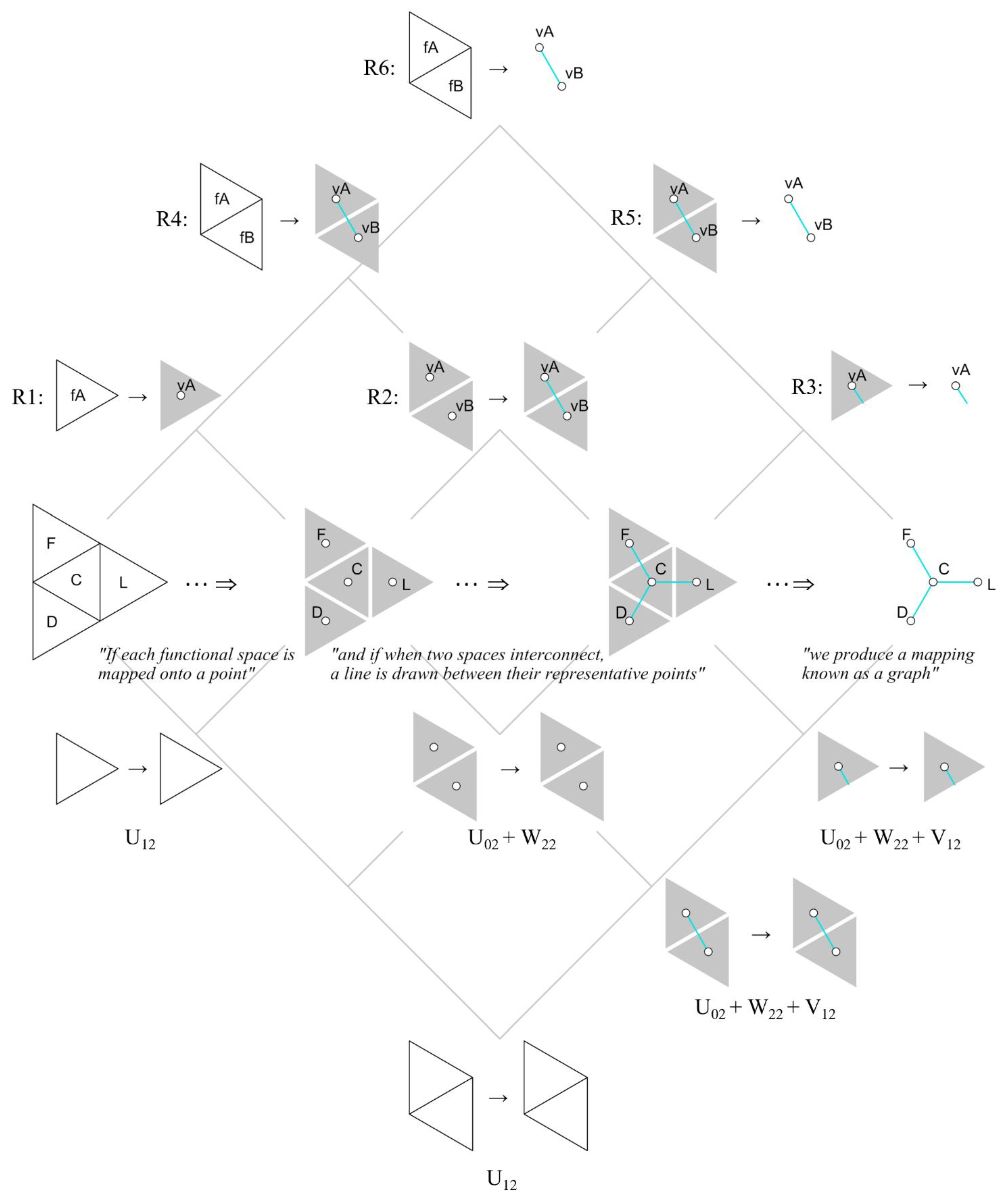
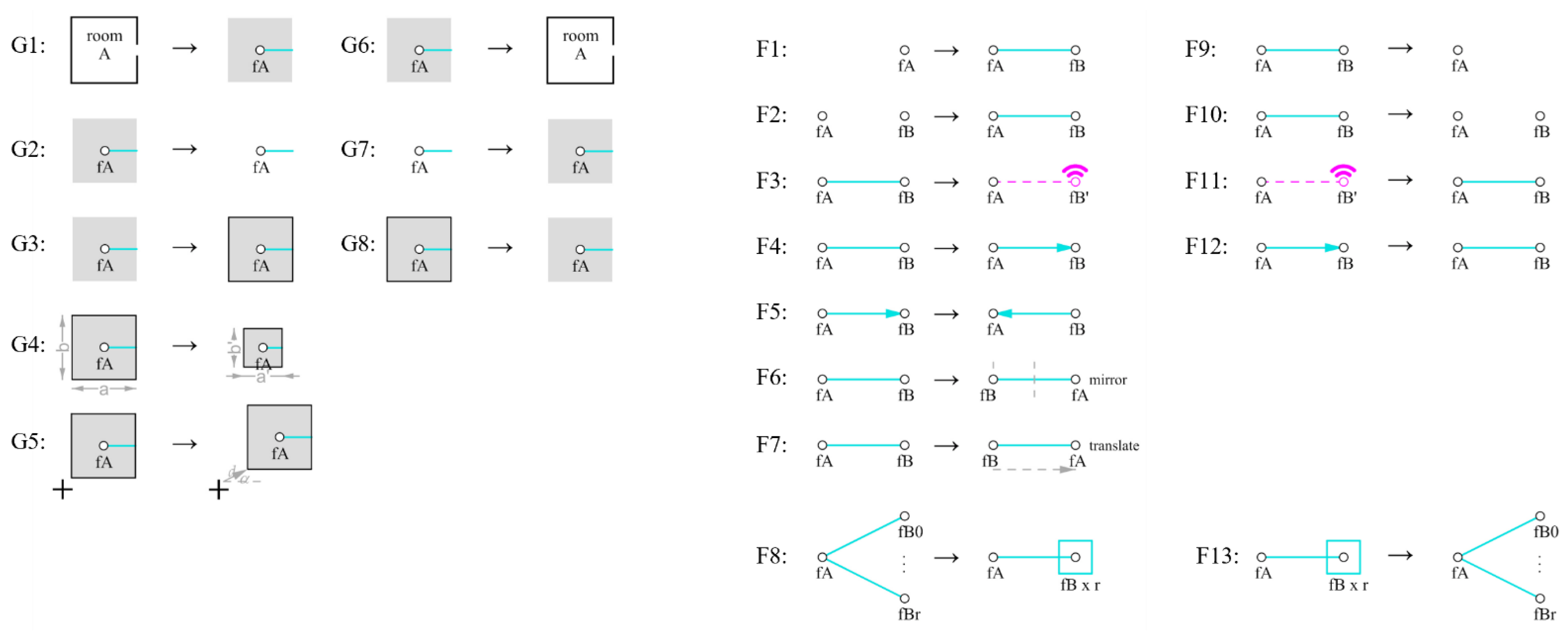
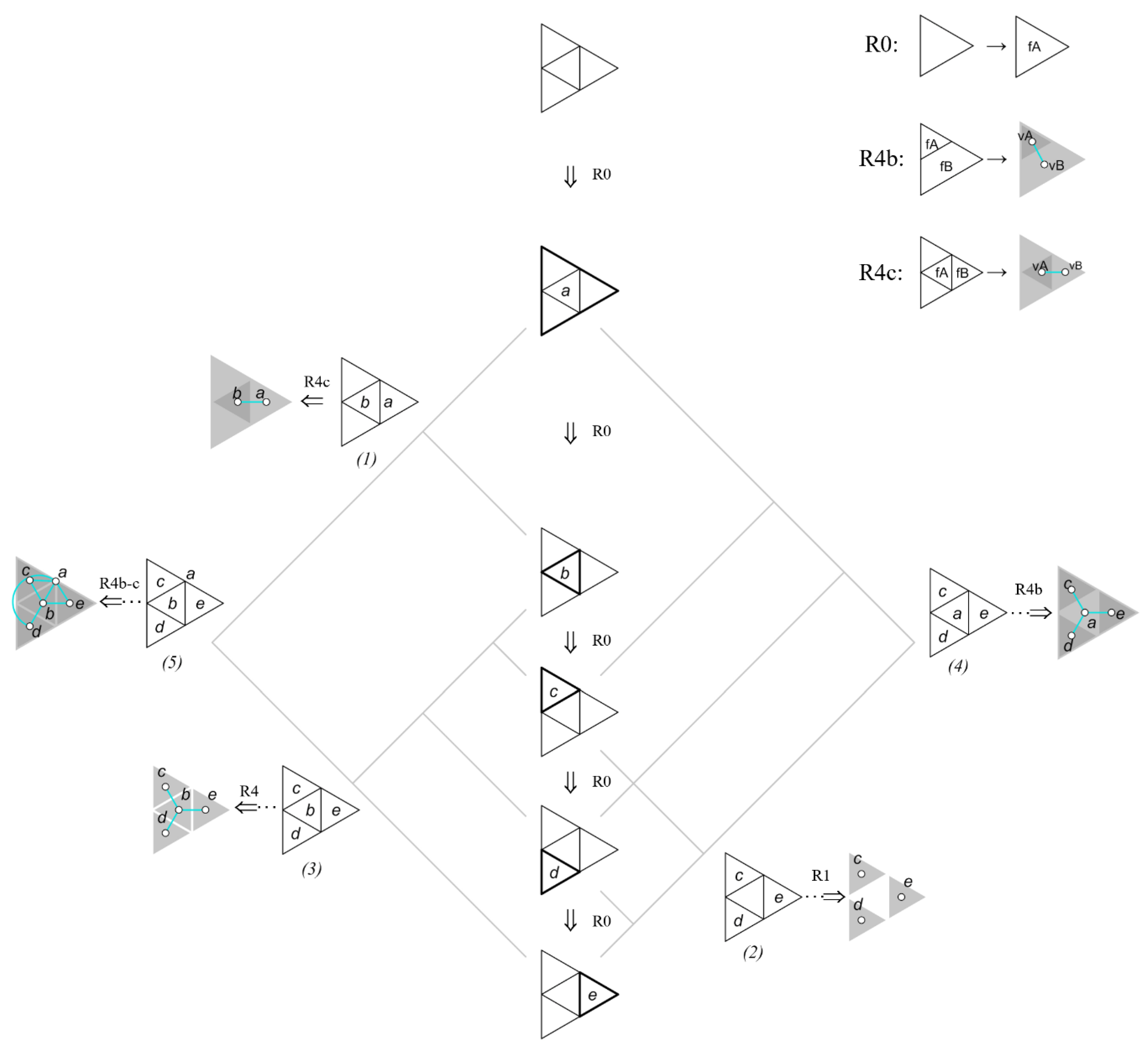
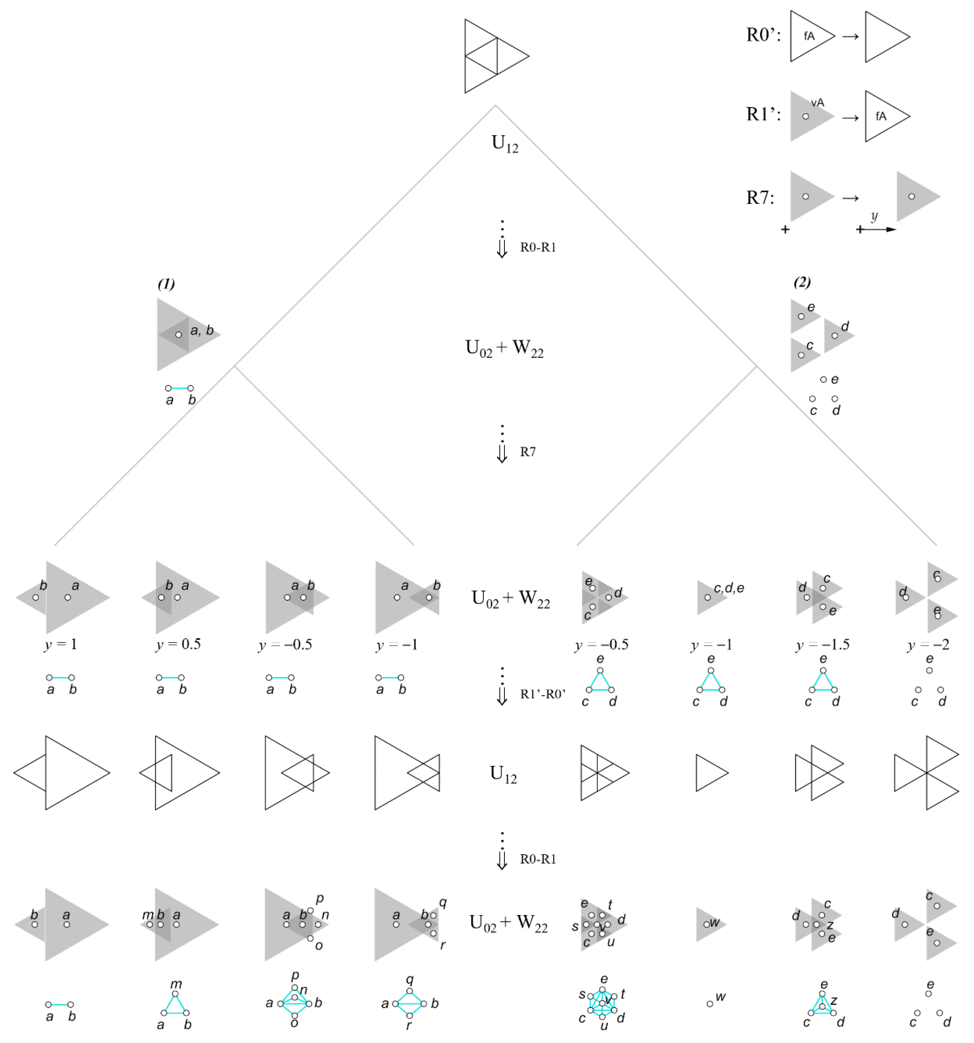
2.6. Shape-to-Graph Rules

Rules G1 to G8 convert a shape into a graph and vice versa. Rule G1 returns a room’s function node, represented by a point, weighted by a plane (tone) representing the room’s boundaries, and labelled by edges to indicate access position. The function name corresponds to the room’s name to indicate the user’s activity (e.g., bedroom for sleeping). Rule G3 returns the weighted node into a shape to enable shape transformation by rule G4 (scaling) or G5 (translation and rotation). When the shape boundary changes, the weight follows. Rule G2 removes the weight and leaves only nodes and edges as a function graph without hinting at the spatial condition. In graph mode, modifications can only be made through functional reconfiguration and their sequence orders (as explained in the subsequent section). Rules G6, G7, and G8 are the inverse of G1, G2, and G3 to convert the graph back to a shape. Rule G7 returns the weight. Rule G8 removes the shape boundary. Rule G6 removes the weight and returns a function node to a room’s shape with its corresponding name. The room’s opening is positioned based on the line label orientation.

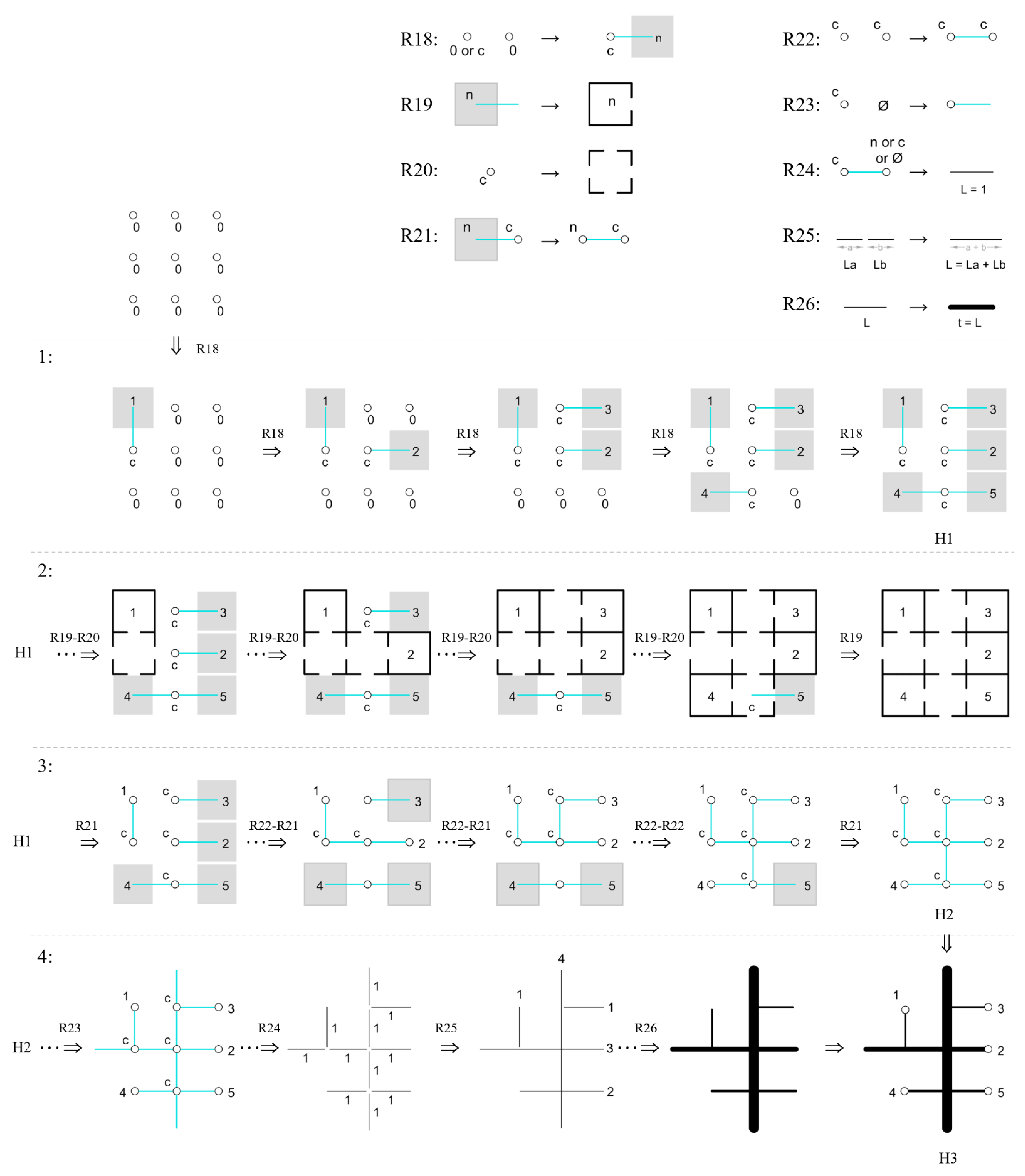
2.7. Graph-to-Graph Rules

Rules F1 and F9 add and remove an activity node in a graph, while rules F2 and F10 add and remove connectivity between nodes. To incorporate virtualisation trends, rule F3, marked with a Wi-Fi symbol, replaces a physical activity with a digital one (e.g., an online check-in), while its inverse (rule F11) returns the digital to a physical activity (e.g., from an online to an in-person meeting). Direction rules F4 and F12 add and remove direction to an edge, while rule F5 reverses the direction. The transformation rules F6 and F7 rearrange the position of the nodes in the graph through translation and reflection (mirroring by node or edge) for the exploration of different functional configurations. Annotation rule F8 is added for graph organisation by grouping the same functions into one (e.g., groups of bedrooms or classrooms), and rule F13 ungroups them. These rules are labelled by the number of elements (r) in a group (F × r). Grouping could be useful in the early design stage, such as in configuring private, public, and utility zones.

3. Case Study

The chosen case studies–hotel and trading spaces–represent a typology that is prone to functional changes. The iteration shows how the functions evolved and were followed by building plan transformation and how alternative building plans can be exercised while preserving functional relations. The case studies are presented in diagrammatic resolution to clarify the functional graph and shape arrangements.

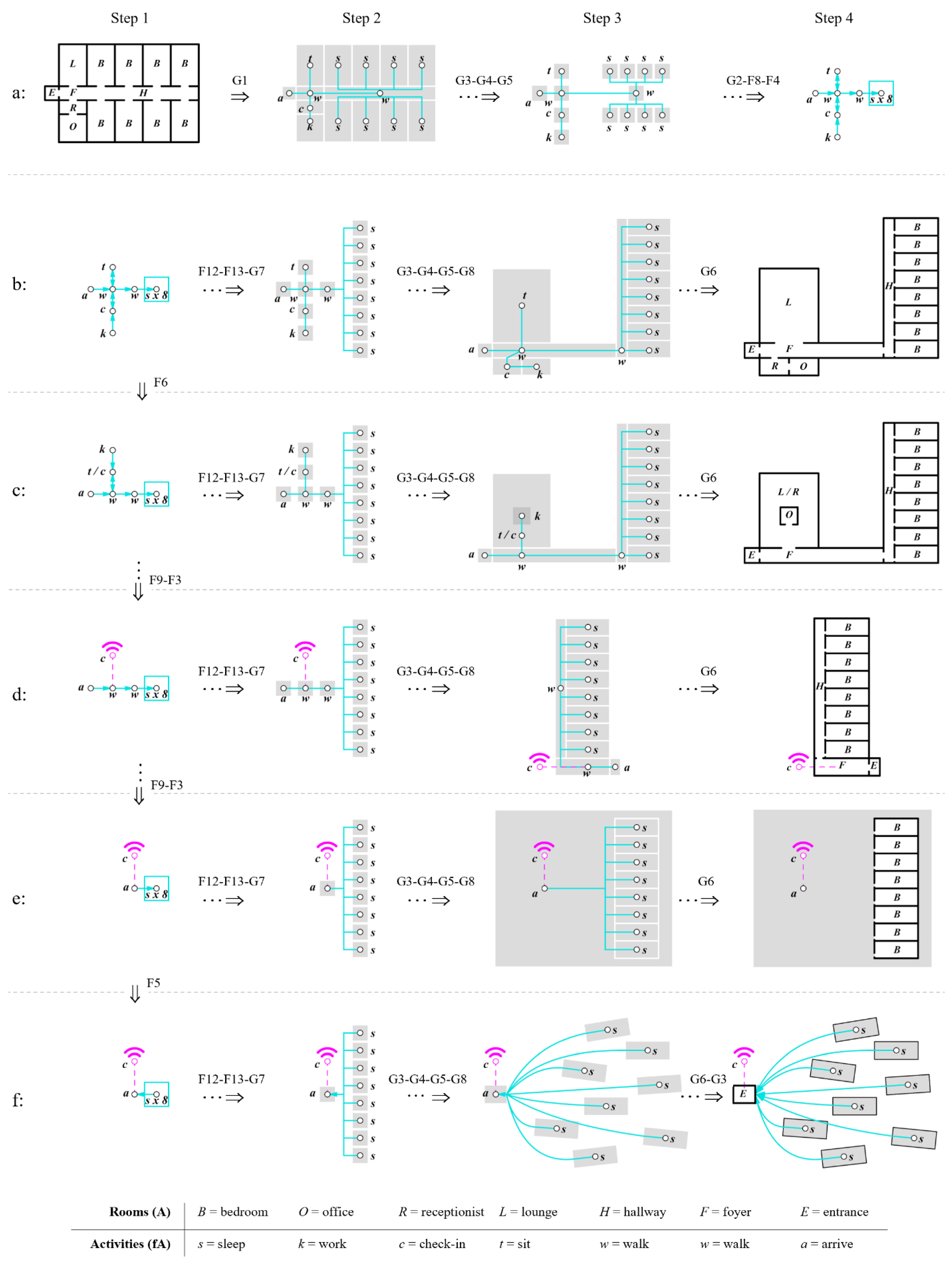
3.1. Case 1: Hotel Lobby

Over the years, the strategies for accommodating travellers have evolved considerably. One significant transformation can be seen in the hotel lobby, which bridges public and private spaces, often coupled with various amenities [53,54,55,56,57]. The lobby features ambassadorial roles for the hotel, ranging from basic functions such as reservation and waiting to perceptual roles for simulating a welcoming place to attract guests. Figure 7 demonstrates how graph and shape rules are computed to examine how a lobby is transformed through amenities and technology. The horizontal iterations show shape-to-graph and graph-to-shape iterations, while the vertical iteration shows a graph-to-graph iteration applied to the first step at each row from Figure 7a–e. The horizontal iteration modifies spatial experience, while the vertical iteration alters the functional sequences.

3.1.1. Shape to Graph—Graph to Shape

Figure 7a shows a shape-to-graph conversion for a simple hotel layout consisting of a waiting lounge, a receptionist desk with an office, and several bedrooms. Given the room and access layout in step 1, labelled with names, rule G1 returns the room’s nodes with the shape weight and edges between the nodes, labelled with activity names in step 2. At this step, both functional relationships and spatial conditions are visible. In step 3, rules G3, G4, and G5 normalise the weight into identical sizes (i.e., squares) and rearrange them to simplify their arrangement. These steps result in a graph, visualised with normalised weights. Step 4 removes the weight with rule G2, leaving only the nodes and edges as a graph. Rule F8 groups nodes of the same activities, and rule F4 adds direction to the edges according to a hotel guest’s flow of activity. The iteration in Figure 7b reverses the graph from Figure 7a (step 4), back to a shape and into a different design. From step one to step two, rule F12 removes the directions of the edges; rule F13 ungroups the bedroom nodes; and rule G7 returns the shape weight for each node. Next, rules G3, G4, and G5 rearrange the nodes by distancing the bedroom nodes from the lobby. Rules G8 and G6 return the boundary shape of the weights. The plan in step 4 is different from the initial plan, yet the graph remains the same. The new arrangement suggests a similar functional experience for the user with a different spatial experience (e.g., a more private bedroom zone).

3.1.2. Graph to Graph—Graph to Shape

The iteration in Figure 7c shows how the sequences of functions are reconfigured. While the resulting plans in step 4 between Figure 7b,c look similar, the functional experience in the lobby is profoundly different. As seen from step 1 in Figure 7b to step 1 in Figure 7c, rule F6 mirrors the check-in and work nodes with the walking (foyer) node as the mirroring axis, resulting in a new graph, where the sitting and check-in nodes have merged, with a work node as their child node. The graph indicates that the area for sitting will also be used for check-in, and the receptionist will approach the sitting guests. The resulting design in step 4 reflects these consequences, where the reception and offices become part of the sitting lounge.
The graph transformation from Figure 7c,d demonstrates a functional and spatial reduction. Rule F9 removes the sitting node, and rule F3 replaces the working and check-in nodes with a virtual node, which practically removes the sitting lounge and the receptionist from the plan. Instead, a guest would check in virtually (e.g., through a sensor, a vending machine, or a mobile device). The resulting graph has two walking nodes, as indicated by a foyer and a corridor in the plan in step 4.
The subsequent two iterations exemplify how a final design and an ongoing design process can coexist in the plan. In the iteration in Figure 7e, rule F9 continues to remove the walking node from the graph in Figure 7d, implying that a dedicated room for walking is no longer necessary. Rule F3 mirrors the virtual nodes with an edge between the arrival and walking nodes. As seen in the output plan in step 4, a corridor is no longer connected to the bedrooms. Instead, while the sleeping nodes have been finalised into bedroom shapes with rule G6, the arrival node remains as a graph with weight. It suggests that the bedrooms’ design is fixed but the arrival position and context are flexible, such as in a capsule hotel in an airport or mall. In step 1 in Figure 7f, the difference with the graph in Figure 7e is subtle, with only the arrow reversing direction by rule F5. Yet, the reversal creates a substantial difference in functional and spatial experience. The arrow suggests that instead of a guest walking into a sleeping node from the arrival node, the sleeping node approaches the guest in the arrival node. After transforming the sleeping node’s position and orientation with rules G3, G4, and G5, the resulting plan in step 4 produces a fixed entrance. Yet, the size and position of the bedroom remain in flexible positions, as indicated by the weighted nodes and directed edges (e.g., floating hotel).
As shown above, the graph iterations not only capture a functional evolution and alternative building plan they also embed different states of a design process in the final operation. Subtracting rules are predominantly used in this case and gradually shrink the graph. Other rule operations can expand the graph for different results to provide spaces for more functions (amenities) with addition rules (Figure 4) or translation rules (Figure 3) to create an overlapping space. Additionally, the number of graph nodes and similar shapes can inform preferences for construction types (e.g., in situ or off-site production). For instance, repetitive functions with identical shapes, such as bedrooms or corridors, can be considered for a prefabricated module, and non-repetitive functions, such as a hotel lounge, might be more suitable for in situ construction.

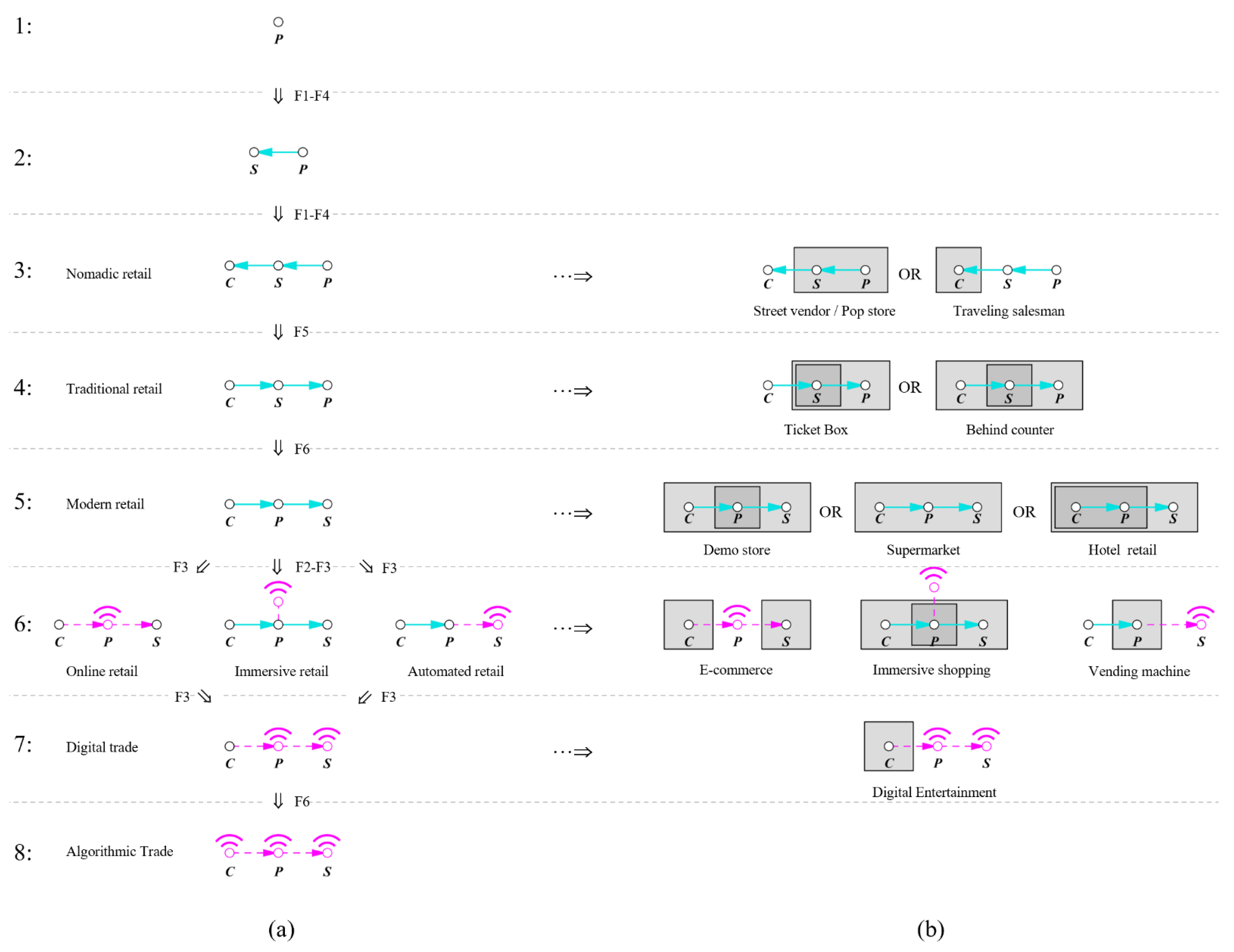
3.2. Case 2: Trading Space

Spatial configuration for trading space has experienced substantial disruption in recent decades, such as in retail, where customers browse and buy products [58,59,60]. Improving customer experiences has been the main goal in the retail industry [61]. This case demonstrates the graph and shape rules to examine function evolution and alternative spatial configuration in trading spaces by generating trade flows based on three basic nodes: the customer, product, and seller. The customer node represents the space where they are present; the product node represents the space for product display; and the seller node represents the space where the transaction occurs. Figure 8 outlined shape rules to generate spatial arrangements for trade flow functional evolution in Figure 9a. The flow transformation is arranged similarly to that of Figure 7, where the vertical iteration (Figure 9a) demonstrates trade flow transformation, and the horizontal iteration in Figure 9b shows the consequences of spatial transformation, as calculated with the rules explained in Figure 8.

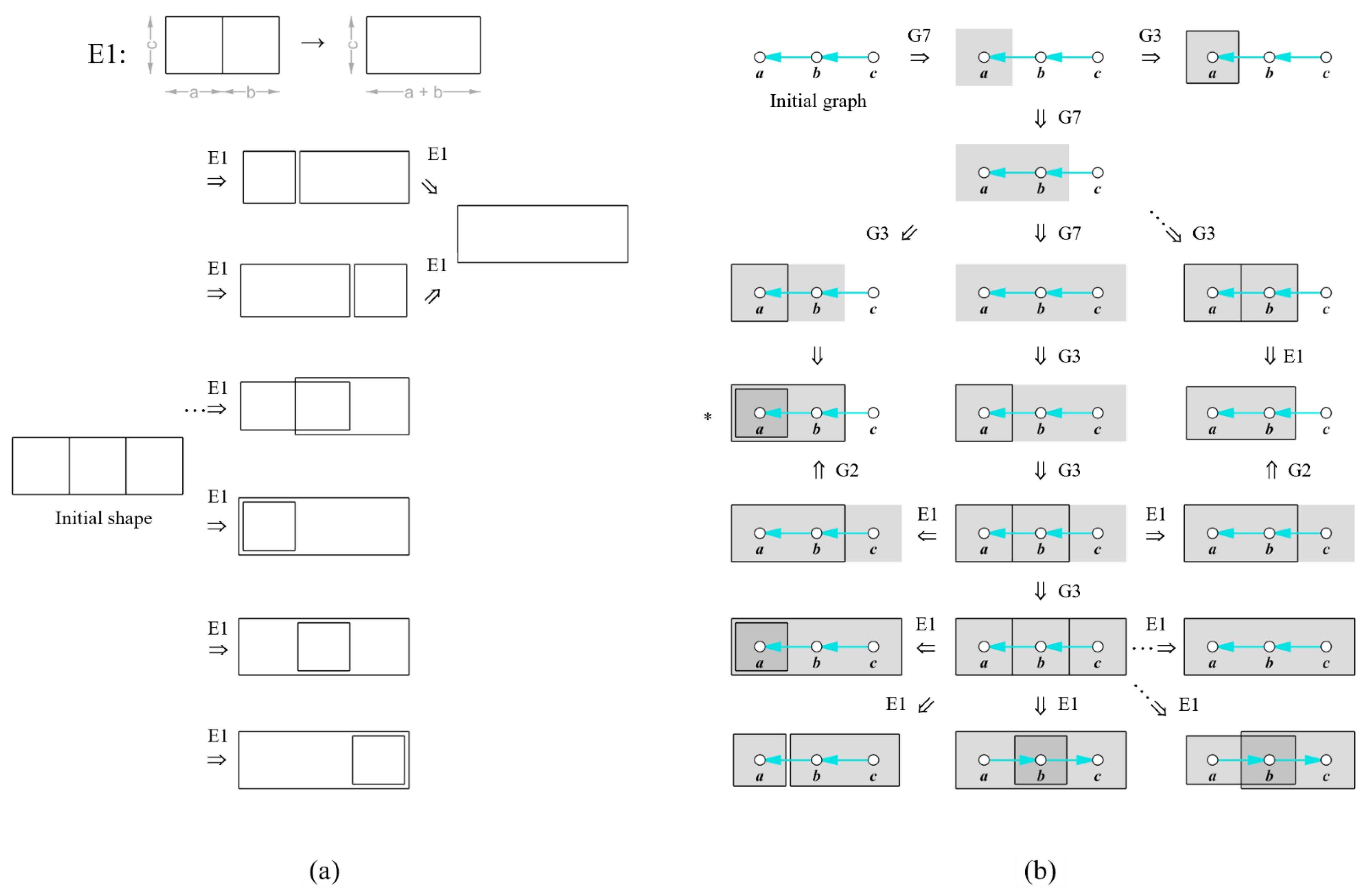
3.2.1. Graph to Graph

Moving vertically from step one to step two in Figure 9a, rules F1 and F4 add a seller node to the product node. In step three, a customer node is added and linked to the seller node with the same rules. This graph can describe a travelling salesman or a street vendor’s trade flows, where the seller brings the product to the customer’s house or public areas in a city. In step four, rule F5 changes the direction of the edge, where the customer node goes to a seller node, which itself goes to the product node. This graph illustrates traditional retail, where the customer visits the seller to buy a product displayed behind or below the counter. Step five uses rule F6 to mirror the product and seller nodes’ positions, allowing the customer to browse the product display directly and then bring the products to the seller for transaction. This swap can illustrate the shift from traditional to modern retail, where customers can browse products directly on display (with RFID tags attached for safety reasons) [62].
The subsequent steps involve rule F3, in which virtual activity replaces physical activity. This rule is applied in step 6a to virtualise the product node into, for instance, a screen (online) display. The customer interacts with the product virtually with the products located in a remote location (e.g., with pick-up or delivery options) or in close proximity to a customer (e.g., a restaurant that uses an app-based menu) [63]. Step 6b adds a virtual function to a physical store to combine digital and physical experiences (e.g., with immersive technology) [64]. Step 6c converts the seller node into a virtual node. It allows a customer to browse the product display physically and perform the transaction online without interacting with the seller, e.g., via a sensor or a self-checkout machine. Step seven virtualises both the product and the seller nodes. This graph illustrates the case of non-physical products (e.g., music or movies), where the seller can sell them online and the customer can purchase them online via a physical outlet (e.g., digital player). In the final step (eight), all the nodes become virtual. This graph can describe a condition where customers and sellers delegate their trading activities digitally for a virtual product (e.g., an automated or algorithmic trading system for shares and crypto) where no physical space is required [65].

3.2.2. Graph to Shape—Shape to Shape

Most of the examples in the cases so far show spatial configuration arranged for a symbolic shape. To demonstrate shape embedding, this case adds rule E1, which combines two adjoining rectangles into one (each can have various lengths and yet have the same height). This rule utilises SG reduction rules to recognise sub-shapes embedded within lines along the rectangles’ boundaries [42,66]. By recognising these lines as sub-shapes, the rule could produce various spatial compositions for a graph with a minimum of transformation rules.
With SG embedding, rule E1 iteration on two adjoining rectangles can generate six rectangular arrangements, two of which can further produce a single rectangle (Figure 8a). With such versatility, rule E1 can be applied to rectangular compositions generated from graph-to-shape rules to exercise possible spatial arrangements for a functional configuration. Figure 8b shows at least 18 possible spatial arrangements for a three-node graph, including a combination of their outputs (*). Some of them indicate functions with separated spaces, while others show functions with overlapped and confined spaces. Additionally, function nodes can be bound by definitive shapes (e.g., walls or partitions) or indicative space marked by weight (e.g., furniture arrangement) or they can be not bound by anything (e.g., outdoor space). The diagrammatic section could inform the decision-making process at a later stage, such as in choosing the structural configuration and envelope system. For instance, shapes with boundaries that face outdoor spaces require treatment to weather the building; shapes that cover more nodes may require a longer span, and a confined shape may be less constrained in the building structure and can be freely articulated.
In a retail context, the rule application is demonstrated in several examples of trading space arrangement for the same trade flow graph. After rules G2, G3, and G7 are applied to the graph in Figure 9a, each node, except for the virtual nodes, has a rectangular weight and shape boundary to represent a diagrammatic section of the space. These rectangles are then applied with rule E1 to generate the different compositions in Figure 9b. For instance, the graph from step three is transformed into two compositions. One is where the seller and the product share the same rectangle, separated from the customer’s, which may illustrate a seller with a non-permanent space (e.g., pop-up stores or street vendors, such as food trucks). The other shows all the customers, sellers, and products sharing the same space (e.g., a salesman selling a product door to door). The graph from step four is transformed into overlapping rectangles, one with a square confined within a rectangle and a customer node on the outside (e.g., a ticket box at a cinema or stadium), another with the seller space separating the space between the customer and the product (e.g., as in a traditional behind-the-counter store). Composition one from step five’s graph shows a product square confined within a rectangle shared by the customer and the seller (e.g., an enclosed space in a demo store, where a customer can experience the product). Composition two from the same graph shows a rectangle shared by all three nodes (e.g., a supermarket), and composition three shows an overlap between customer space and seller space (e.g., a retail store within a hotel, where the customer can experience the seller’s products during their stay). In step six, one composition shows two squares separated by a virtual node, indicating they are physically distant (e.g., e-commerce); one composition mimics a demo store with a virtual node (e.g., AR/VR experience in-store); and the last composition shows a customer accesses the product physically while the seller is virtually connected (e.g., a vending machine). The last output from step seven only shows one rectangle, representing a space where only the customer is present physically (e.g., digital entertainment).

4. Results

The outputs from the above cases show several highlights from the interplay between the graph and shape rule, including the roles of shape, label, and weight.

4.1. Shape-Driven: New Spatial Experience for the Same Function

First, the experiments show how the iterations for graph and shape rules can work in tandem in a design process. The initial iterations with a simple hotel plan show different designs generated from the same graph, echoing the lessons from the revisited study. The dual presence of graphs and weighted shapes can assist in simultaneously evaluating early spatial and functional conditions. The use of graph transformation rules helps to quickly assemble different spatial arrangements (e.g., within the site). Additionally, the directed edges in the graph can ensure that the resulting room layout does not compromise the required access and sequences, and the weighted nodes indicate the intended sizes and proximity between rooms. Generating a functional–spatial graph schematically could clarify functional evolution and how it transforms building plans, as well as exercise alternative building plans while preserving functional relations.

4.2. Graph-Driven: New Functional Experience with Similar Shapes

Second, the iterations from the cases show that creative spatial solutions can start at functional iteration before shape articulations. The hotel lobby case demonstrated how graph rules generate various functional sequences and configurations. Some rules, such as the erasing and virtualisation rules, produce the expected results with disappearing functions and their respective spaces. Other rules produced rather unexpected effects, such as the mirroring rules, which could merge functions, and the reversing of a rule, which creates profound experiential changes by swapping the sequence direction. While it appears simple, a change in flow direction could help improve users’ experiences, e.g., by providing a space designed for staff to approach guests for check-in. Some iteration in the cases also suggests that differences in user experience can be achieved by modifying the order of rules in the iteration and that the final design can be set without having all the shapes fixed. Leaving some shapes at their weighted graph state could provide alternative means for the users’ flow of activities.

4.3. Graph- and Shape-Driven: New Functional and Spatial Experience

Third, shape embedding can help to generate a profound spatial impact. As demonstrated in the second case, rule iteration with shape embedding can produce different spatial configurations to accommodate the same trade flow activities, as seen in the trading space case.

4.4. Rule Characteristics in Graph-to-Shape Iteration

The study also notices different rule characteristics in generating graphs to shapes pertinent to the building design. The substitution rule is more deterministic as it initiates a shape from a node and an edge into a component (e.g., opening), and its geometry could be dominating in a building’s design language. The subdivision rule is constraining as the iteration typically goes inward and ensures that spaces for functions are multiplied inside an initial shape (e.g., a site boundary or a building envelope). Some additive rules are expansive and less sensitive to boundaries when populating a shape unless they are accompanied by overlapping rules [67,68,69,70]. The identity rule is intriguing as it invites opportunities to explore what shapes and rules can do in graph-to-shape translation. For instance, it allows the same shape to be implemented across stages to maintain a design language, namely from the functional to the structural configuration stages. In Sundt house, the triangle for functional arrangement is also applied for columns profiles and column positions, while in the Jester house, the circles extruded into the walls and columns. This also suggests that consistency throughout function, design, and construction can be achieved if graph-to-shape iteration is aligned with, or generated over, structural grids, e.g., the triangular and rectilinear–circular grids.

5. Discussion

This study revisited early studies on graph and shape in computation design to examine their compatibility and to interpret a set of rules to map a function graph from design and generate a design from a function graph that mediates spatial and functional relationships. Two cases demonstrated the lessons learned from the revisited studies on how graph and shape rules can create sequences of functions in pairs with spatial development.
The experiments shown are predominantly run with the combinatorial operation, presented with schematic resolutions, and have yet to utilise a benchmarking system to evaluate the output performance in detail. There are other features in SG visual calculation and SS evaluation systems that have yet to be tested, such as isovist and depth measurement with JPG. Incorporating these other features could help increase design variety and separate the useful and useless results. Further studies could include resolution enhancement of the diagrammatic outputs with tools such as those mentioned in [36,38,71,72], and function descriptions can be organised into an ontological structure in semantic modelling [73,74,75].
Nevertheless, the main principles of operating shape and graph calculations have been outlined and demonstrated in this paper. The generative rules can help to analyse functional evolution as well as to synthesise different functional sequences and their alternative building plans to venture into different typologies, which, in Lionel March’s words, ‘minimises prejudice and maximises choice’. Shape and graph integration can show how a function within a building, such as a hotel or a retail establishment, evolves and shrinks, as well as what alternatives exist for creating new experiences or new business models.

Funding

This research received no external funding.

Data Availability Statement

Not applicable.

Conflicts of Interest

The author declares no conflict of interest.

References

  1. Boddy, N. Australia COVID: Office occupancy rates go backwards for the first time in six months. Financial Review, 11 August 2022. [Google Scholar]
  2. Zettl, M. Office buildings are still less than 50% occupied. Who should worry? Forbes, 29 November 2022. [Google Scholar]
  3. Duffy, F. Office buildings and organisational change. In Buildings and Society; Routledge: London, UK, 2003; pp. 147–163. [Google Scholar]
  4. WAF. World Architecture Festival 2022 Winners Homepage. Available online: https://www.worldarchitecturefestival.com/waf2023/en/page/waf-2022 (accessed on 5 December 2022).
  5. Amoils, J. The evolving workplace: Where to next in a post-pandemic world? CRE Real Estate Issues 2021, 45, 1–10. [Google Scholar]
  6. Duchene, P. The evolving workplace. Forbes, 12 March 2019. [Google Scholar]
  7. Sweeney, S. Post-Pandemic Utilization of Office to Residential Adaptive Reuse Strategies in Cities. Master’s Thesis, University of North Carolina, Chapel Hill, NC, USA, 6 April 2021. [Google Scholar] [CrossRef]
  8. RIBA. RIBA Plan of Work 2020 Overview; RIBA Publications: London, UK, 2020. [Google Scholar]
  9. American Institute of Architects, The Architect’s Handbook of Professional Practice; John Wiley & Sons, Incorporated: New York, NY, USA, 2013.
  10. Hillier, B.; Leaman, A.; Stansall, P.; Bedford, M. Space syntax. Environ. Plan. B Plan. Des. 1976, 3, 147–185. [Google Scholar] [CrossRef]
  11. Kim, Y.O.; Kim, J.Y.; Yum, H.Y.; Lee, J.K. A study on mega-shelter layout planning based on user behavior. Buildings 2022, 12, 1630. [Google Scholar] [CrossRef]
  12. Zhang, X.; Cui, T. Evolution process of scientific space: Spatial analysis of three groups of laboratories in history (16th–20th century). Buildings 2022, 12, 1909. [Google Scholar] [CrossRef]
  13. Lee, J.H.; Kim, Y.S. Rethinking art museum spaces and investigating how auxiliary paths work differently. Buildings 2022, 12, 248. [Google Scholar] [CrossRef]
  14. Azizi, V.; Usman, M.; Sohn, S.S.; Schwartz, M.; Moon, S.; Faloutsos, P.; Kapadia, M. The role of latent representations for design space exploration of floorplans. Simulation 2022, 375497221115734. [Google Scholar] [CrossRef]
  15. Stiny, G.; Gips, J. Shape grammars and the generative specification of painting and sculpture. In Proceedings of the IFIP Congress 71, Ljubljana, Yugoslavia, 23–28 August 1971; pp. 125–135. [Google Scholar]
  16. Belčič, A.; Eloy, S. Architecture for community-based ageing—A shape grammar for transforming typical single-family houses into older people’s cohousing in Slovenia. Buildings 2023, 13, 453. [Google Scholar] [CrossRef]
  17. Flemming, U. More than the sum of parts: The grammar of Queen Anne houses. Environ. Plan. B Plan. Des. 1987, 14, 323–350. [Google Scholar] [CrossRef]
  18. Cagdas, G. A shape grammar: The language of traditional Turkish houses. Environ. Plan. B Plan. Des. 1996, 23, 443–464. [Google Scholar] [CrossRef]
  19. Colakoglu, B. Design by grammar: An interpretation and generation of vernacular Hayat houses in contemporary context. Environ. Plan. B Plan. Des. 2005, 32, 141–149. [Google Scholar] [CrossRef]
  20. Yousefniapasha, M.; Teeling, C.; Rollo, J.; Bunt, D. Shape grammar, culture, and generation of vernacular houses (a practice on the villages adjacent to rice fields of Mazandaran, in the north of Iran). Environ. Plan. B Urban Anal. City Sci. 2021, 48, 94–114. [Google Scholar] [CrossRef]
  21. Erem, Ö.; Ermiyagil, M.S.A. Adapted design generation for Turkish vernacular housing grammar. Environ. Plan. B Plan. Des. 2016, 43, 893–919. [Google Scholar] [CrossRef]
  22. Haakonsen, S.; Rønnquist, A.; Labonnote, N. Fifty years of shape grammars: A systematic mapping of its application in engineering and architecture. Int. J. Arch. Comput. 2022, 14780771221089882. [Google Scholar] [CrossRef]
  23. Ehrig, H.; Pfender, M.; Schneider, H.J. Graph-grammars: An algebraic approach. In 14th Annual Symposium on Switching and Automata Theory (swat 1973); IEEE: Piscataway, NJ, USA, 1973; pp. 167–180. [Google Scholar]
  24. Rozenberg, G. Handbook of Graph Grammars and Computing by Graph Transformation; World Scientific: Singapore, 1997; Volume 1. [Google Scholar]
  25. Voss, C.; Petzold, F.; Rudolph, S. Graph transformation in engineering design: An overview of the last decade. Artif. Intell. Eng. Des. Anal. Manuf. 2023, 37, e5. [Google Scholar] [CrossRef]
  26. Weber, R.E.; Mueller, C.; Reinhart, C. Automated floorplan generation in architectural design: A review of methods and applications. Autom. Constr. 2022, 140, 104385. [Google Scholar] [CrossRef]
  27. Nourian, P.; Azadi, S.; Oval, R. Generative design in architecture: From mathematical optimization to grammatical customization. In Computational Design and Digital Manufacturing; Springer: Berlin/Heidelberg, Germany, 2023; pp. 1–43. [Google Scholar] [CrossRef]
  28. Heitor, T.V.; Duarte, J.P.; Pinto, R.M. Combing grammars and space syntax: Formulating, generating and evaluating designs. Int. J. Arch. Comput. 2004, 2, 491–515. [Google Scholar] [CrossRef]
  29. Eloy, S.; Guerreiro, R. Transforming housing typologies. Space syntax evaluation and shape grammar generation. Arq. Urb. 2016, 15, 86–114. [Google Scholar]
  30. Lee, J.H.; Ostwald, M.J.; Gu, N. A Justified Plan Graph (JPG) grammar approach to identifying spatial design patterns in an architectural style. Environ. Plan. B Urban Anal. City Sci. 2016, 45, 67–89. [Google Scholar] [CrossRef] [Green Version]
  31. Lee, J.H.; Ostwald, M.J.; Gu, N. A Combined plan graph and massing grammar approach to frank lloyd wright’s prairie architecture. Nexus Netw. J. 2017, 19, 279–299. [Google Scholar] [CrossRef] [Green Version]
  32. Lee, J.H.; Ostwald, M.; Gu, N. A syntactical and grammatical approach to architectural configuration, analysis and generation. Arch. Sci. Rev. 2015, 58, 189–204. [Google Scholar] [CrossRef]
  33. Etintaş, M.F.; Erem, N.Ö. Outpatient clinic design through rule based design methods. Eskişeh Tech. Univ. J. Sci. Technol.-Appl. Sci. Eng. 2022, 23, 156–171. [Google Scholar]
  34. Grasl, T.; Economou, A. From topologies to shapes: Parametric shape grammars implemented by graphs. Environ. Plan. B: Plan. Des. 2013, 40, 905–922. [Google Scholar] [CrossRef] [Green Version]
  35. Lima, F.; Brown, N.C.; Duarte, J.P. Optimizing urban grid layouts using proximity metrics. In Artificial Intelligence in Urban Planning and Design; Elsevier: Amsterdam, The Netherlands, 2022; pp. 181–200. [Google Scholar]
  36. Hong, T.-C.K.; Economou, A. Implementation of shape embedding in 2D CAD systems. Autom. Constr. 2023, 146, 104640. [Google Scholar] [CrossRef]
  37. Schaffranek, R.; Vasku, M. Space syntax for generative design: On the application of a new tool. In Proceedings of the Ninth International Space Syntax Symposium, Seoul, Republic of Korea, 31 October–3 November 2013. [Google Scholar]
  38. Stouffs, R. A Multi-formalism Shape Grammar Interpreter. In Computer-Aided Architectural Design. Design Imperatives Future Now; Gerber, D., Pantazis, E., Bogosian, B., Nahmad, A., Miltiadis, C., Eds.; Springer: Singapore, 2022; Volume 1465, pp. 268–287. [Google Scholar] [CrossRef]
  39. Lambe, N.R.; Dongre, A.R. A shape grammar approach to contextual design: A case study of the Pol houses of Ahmedabad, India. Environ. Plan. B Urban Anal. City Sci. 2019, 46, 845–861. [Google Scholar] [CrossRef]
  40. Veloso, P.; Celani, G.; Scheeren, R. From the generation of layouts to the production of construction documents: An application in the customization of apartment plans. Autom. Constr. 2018, 96, 224–235. [Google Scholar] [CrossRef]
  41. Vardouli, T. Skeletons, Shapes, and the Shift from Surface to Structure in Architectural Geometry. Nexus Netw. J. 2020, 22, 487–505. [Google Scholar] [CrossRef]
  42. Stiny, G. Shape: Talking about Seeing and Doing; The MIT Press: Cambridge, MA, USA, 2006. [Google Scholar]
  43. Stiny, G. Shapes of Imagination: Calculating in Coleridge’s Magical Realm; MIT Press: Cambridge, MA, USA, 2022. [Google Scholar]
  44. Hillier, B. The nature of the artificial: The contingent and the necessary in spatial form in architecture. Geoforum 1985, 16, 163–178. [Google Scholar] [CrossRef] [Green Version]
  45. Hillier, B. Space Is the Machine: A Configurational Theory of Architecture; Cambridge University Press: Cambridge, MA, USA, 1996; p. 463. [Google Scholar]
  46. Coates, P. Programming Architecture, 1st ed.; Routledge: London, UK, 2010. [Google Scholar]
  47. Alexander, C. Notes on the Synthesis of Form; Harvard University Press: Cambridge, MA, USA, 1964; Volume 5. [Google Scholar]
  48. March, L.; Steadman, P. The Geometry of Environment. An Introduction to Spatial Organization in Design; MIT Press: Cambridge, MA, USA, 1974. [Google Scholar]
  49. Muslimin, R. Ethnocomputation: An Inductive Shape Grammar on Toraja Glpyh. In Computer-Aided Architectural Design. Future Trajectories; Çağdaş, G., Özkar, M., Gül, L.F., Gürer, E., Eds.; Springer: Singapore, 2017; Volume 724, pp. 329–347. [Google Scholar] [CrossRef]
  50. Stiny, G. What rule(s) should I use? Nexus Netw. J. 2011, 13, 15–47. [Google Scholar] [CrossRef] [Green Version]
  51. Kotsopoulos, S.D. Design without rigid rules. In Design Computing and Cognition’20; Springer: Berlin/Heidelberg, Germany, 2022; pp. 107–128. [Google Scholar]
  52. Lee, J.H.; Ostwald, M.J.; Gu, N. Combining space syntax and shape grammar to investigate architectural style. In Proceedings of the Ninth International Space Syntax Symposium, Seoul, Republic of Korea, 31 October–3 November 2013; Sejong University: Seoul, Republic of Korea, 2013. [Google Scholar]
  53. Bowie, D. Innovation and 19th century hotel industry evolution. Tour. Manag. 2018, 64, 314–323. [Google Scholar] [CrossRef]
  54. Li, L.; Lu, L.; Xu, Y.; Sun, X. The spatiotemporal evolution and influencing factors of hotel industry in the metropolitan area: An empirical study based on China. PLoS ONE 2020, 15, e0231438. [Google Scholar] [CrossRef]
  55. Murphy, J.; Schegg, R.; Olaru, D. Investigating the evolution of hotel internet adoption. Inf. Technol. Tour. 2006, 8, 161–177. [Google Scholar] [CrossRef] [Green Version]
  56. James, K.J.; Sandoval-Strausz, A.K.; Maudlin, D.; Peleggi, M.; Humair, C.; Berger, M.W. The hotel in history: Evolving per-spectives. J. Tour Hist. 2017, 9, 92–111. [Google Scholar] [CrossRef]
  57. MacDonald, R. Urban hotel: Evolution of a hybrid typology. Built Environ. 1978, 2000, 142–151. [Google Scholar]
  58. Gauri, D.K.; Jindal, R.P.; Ratchford, B.; Fox, E.; Bhatnagar, A.; Pandey, A.; Navallo, J.R.; Fogarty, J.; Carr, S.; Howerton, E. Evolution of retail formats: Past, present, and future. J. Retail. 2021, 97, 42–61. [Google Scholar] [CrossRef]
  59. Miotto, A.P.; Parente, J.G. Retail evolution model in emerging markets: Apparel store formats in Brazil. Int. J. Retail. Distrib. Manag. 2015, 43, 242–260. [Google Scholar] [CrossRef]
  60. Quartier, K. Retail design: What’s in the name? In Retail Design; Routledge: London, UK, 2016; pp. 39–56. [Google Scholar]
  61. Bonfrer, A.; Chintagunta, P.; Dhar, S. Retail store formats, competition and shopper behavior: A Systematic review. J. Retail. 2022, 98, 71–91. [Google Scholar] [CrossRef]
  62. Stobart, J. A history of shopping: The missing link between retail and consumer revolutions. J. Hist. Res. Mark. 2010, 2, 342–349. [Google Scholar] [CrossRef] [Green Version]
  63. Stieninger, M.; Gasperlmair, J.; Plasch, M.; Kellermayr-Scheucher, M. Identification of innovative technologies for store-based retailing—An evaluation of the status quo and of future retail practices. Procedia Comput. Sci. 2021, 181, 84–92. [Google Scholar] [CrossRef]
  64. Hilken, T.; Chylinski, M.; Keeling, D.I.; Heller, J.; Ruyter, K.; Mahr, D. How to strategically choose or combine augmented and virtual reality for improved online experiential retailing. Psychol. Mark. 2021, 39, 495–507. [Google Scholar] [CrossRef]
  65. Treleaven, P.; Galas, M.; Lalchand, V. Algorithmic trading review. Commun. ACM 2013, 56, 76–85. [Google Scholar] [CrossRef]
  66. Kristic, D. Diagonal decompositions of shapes and their algebras. Artif. Intell. Eng. Des. Anal. Manuf. 2022, 36, e10. [Google Scholar] [CrossRef]
  67. Caneparo, L. Semantic knowledge in generation of 3D layouts for decision-making. Autom. Constr. 2022, 134, 104012. [Google Scholar] [CrossRef]
  68. Grasl, T. Transformational palladians. Environ. Plan. B Plan. Des. 2012, 39, 83–95. [Google Scholar] [CrossRef]
  69. Duarte, J.P. Customizing Mass Housing: A Discursive Grammar for Siza’s Malagueira Houses. Ph.D. Dissertation, Massachusetts Institute of Technology, Cambridge, MA, USA, 2001. [Google Scholar]
  70. Stiny, G. Ice-ray: A note on the generation of Chinese lattice designs. Environ. Plan. B Plan. Des. 1977, 4, 89–98. [Google Scholar] [CrossRef]
  71. Okhoya, V.W.; Bernal, M.; Economou, A.; Saha, N.; Vaivodiss, R.; Hong, T.-C.K.; Haymaker, J. Generative workplace and space planning in architectural practice. Int. J. Arch. Comput. 2022, 20, 645–672. [Google Scholar] [CrossRef]
  72. Al-Jokhadar, A.; Jabi, W. Spatial reasoning as a syntactic method for programming socio-spatial parametric grammar for vertical residential buildings. Archit. Sci. Rev 2020, 63, 135–153. [Google Scholar] [CrossRef]
  73. Fernandes, P.A. Space syntax with prolog. In Proceedings of the 13th Space Syntax Symposium, Bergen, Norway, 20–24 June 2022. [Google Scholar]
  74. Andaroodi, E.; Andres, F.; Einifar, A.; Lebigre, P.; Kando, N. Ontology-based shape-grammar schema for classification of caravanserais: A specific corpus of Iranian Safavid and Ghajar open, on-route samples. J. Cult. Heritage 2006, 7, 312–328. [Google Scholar] [CrossRef]
  75. Grobler, F.; Aksamija, A.; Kim, H.; Krishnamurti, R.; Yue, K.; Hickerson, C. Ontologies and shape grammars: Communication between knowledge-based and generative systems. In Design Computing and Cognition ’08; Gero, J.S., Goel, A.K., Eds.; Springer: Dordrecht, The Netherlands, 2008; pp. 23–40. [Google Scholar]
Figure 1. Shape rules induced from March and Steadman statements for the Sundt house plan. The initial shape represents the family (F), dining (D), and living room (L) zones, with the circulation (C) in between.
Buildings 13 00869 g001
Figure 2. Different graphs are derived from one shape by decomposition.
Buildings 13 00869 g002
Figure 3. Comparison between graphs derived from discrete shape transformation (middle) and embedding on continuous shapes (bottom). The description indicates their operating algebras.
Buildings 13 00869 g003
Figure 4. Rule schema, adjacency graph rules, and shape rules (a), with their rule iteration on regenerating plans of the Vigo Sundt house (b) and the Ralph Jester house (c). Labels a and b are replaced by names outlined in the list of descriptions Dmn (d).
Buildings 13 00869 g004
Figure 5. Shape rules (R18–R25) and their iterations to regenerate Hillier’s laws for the construction of spatial orders (H1) in iteration one (1), laws from society to space (H2) in iteration three (3), and laws from space to society (H3) in iteration four (combined with graph H2) (4). Iteration two converts graph H1 into a plan (2).
Buildings 13 00869 g005
Figure 6. A set of shape and graph rules from revisiting studies.
Buildings 13 00869 g006
Figure 7. Graph and shape rule iterations for a hotel lobby (af). Graph-to-graph iteration is shown in the vertical direction (left-hand column) and graph-to-shape iteration in the horizontal direction.
Buildings 13 00869 g007
Figure 8. Reduction rules for adjacent rectangles and example iterations (a) with their application graph-to-shape rules (b).
Buildings 13 00869 g008
Figure 9. Different trade flow and retailing types produced from graph-to-graph iteration (a) and examples of spatial arrangement presented with diagrammatic sections (b). Nodes P = product, S = seller, and C = customer. The wi-fi symbols indicate a virtual function.
Buildings 13 00869 g009
Table 1. Glossary. Readers can find further information on this terminology in [15,42,43] for SG and [10,44,45] for SS.
TerminologyDefinition
ShapeA set shape of i dimensions arranged in j-dimensional space within an algebra Uij, where j- refers to 0-, 1-, 2- or 3- dimensional space, and i- refers to 0 for points, 1 for lines, 2 for planes, and 3 for solids.
LabelA mark to define shape Uij orientation and position by using a shape in algebra Vij (e.g., points (V0j), lines (V1j), or planes (V2j)) or symbols (e.g., with a letter or number).
WeightA graphical property associated with shape Uij in algebra Wij; for instance, a point (U0j) can be weighted with a plane (W2j), a line (U1j) weighted with thickness (W1j), or a plane (U2j) weighted with tones (W2j). In the figures, plane weight is shown in a grey tone and line weight with a black colour.
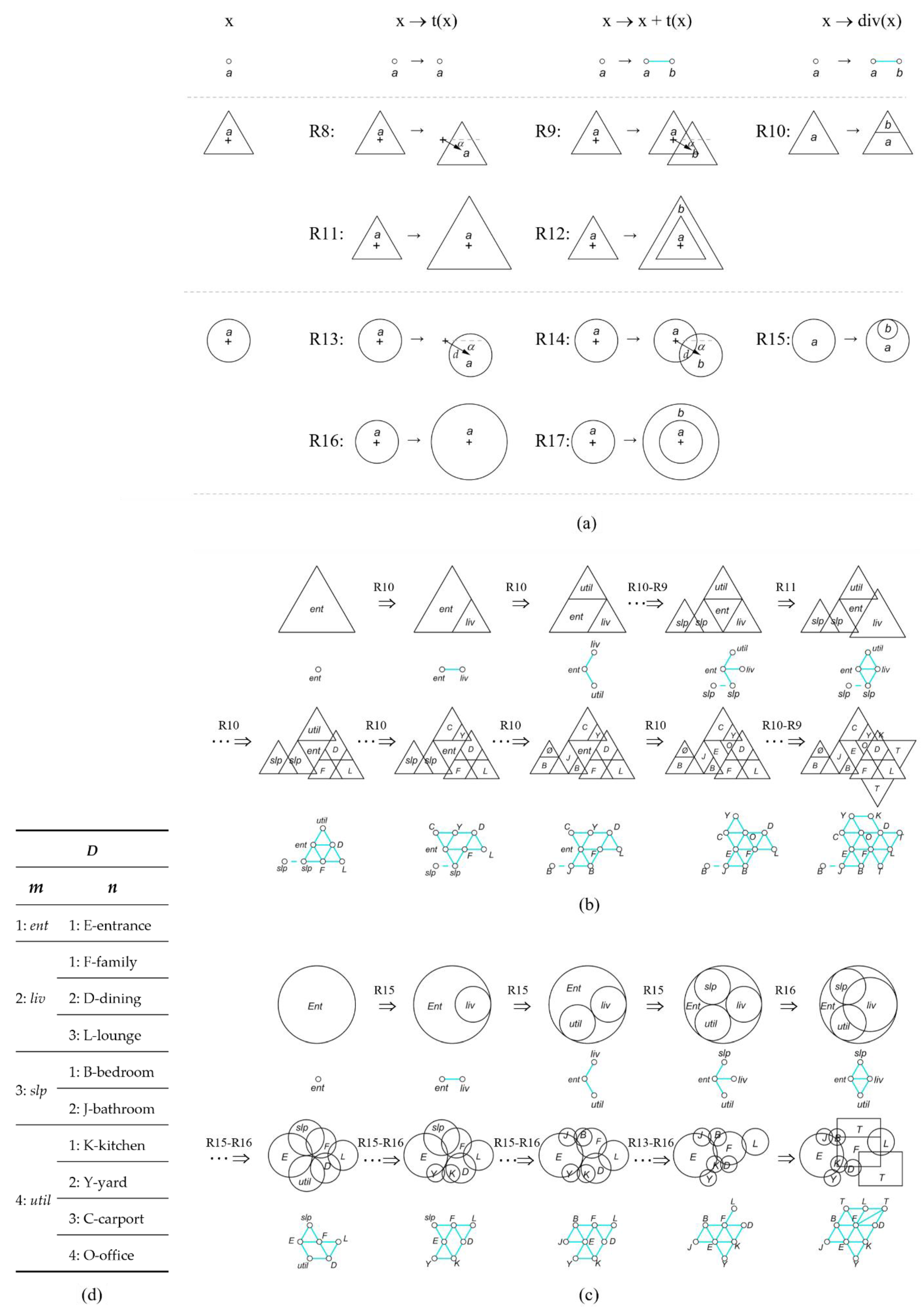
Shape ruleA mapping function (R) to transform shape A into shape B in format R: A → B. Given a shape C, a formula (C-t(A)) + t(B) applies if there is a transformation of shape A or t(A) in shape C.
Rule computationA step-by-step shape rule iteration application whenever a shape matches the left-hand shape of a rule, noted by a double arrow, e.g., C0 ⇒ C1 ⇒ C2 … ⇒ Cn, where shapes C0 to Cn mark the output shapes from the previous step as the input shape for the next step. The three dots […] indicate multiple rules applied in one step (nested between steps).
Rule schemaAn assignment function in format x → y that assigns a predicate shape as the values for variable x and y with assignment g, such that g(x) → g(y) would compose a shape rule A → B.
Shape descriptionA set of descriptions (D) to describe a context for applying shape rules (G) (e.g., a spatial, functional context), assigned with a description function h: LG → D.
GraphA set of nodes (V), such as nodes {a, b, c, d}, connected by a set of edges (E), such as ((a, b), (b, c), (c, d), (d, e)), such that graph G = (V, E). In SS, nodes in the graph usually denote spaces (e.g., streets, rooms, or corridors), and the lines represent the connection or intersection between pairs of spaces. To distinguish the edge from a line in U1j, the edges are coloured cyan.
Disclaimer/Publisher’s Note: The statements, opinions and data contained in all publications are solely those of the individual author(s) and contributor(s) and not of MDPI and/or the editor(s). MDPI and/or the editor(s) disclaim responsibility for any injury to people or property resulting from any ideas, methods, instructions or products referred to in the content.

