Abstract
Raising the final contract cost (FCC) is a significant risk for project owners. This study hypothesizes that the factors that cause owner’s cost estimation (OCE) accuracy and FCC changes share the same causes, and a case study confirmed that the two variables (OCE and FCC) could be correlated. Accordingly, this study aims to develop a forecast model to predict FCC on the basis of the initial OCE, which has not been studied previously. This study utilized data from 34 Saudi Arabian projects. Two linear regression models developed the data, and the square root function transformed the data. Moreover, the artificial neural network (ANN) model was developed after data standardization using Zavadskas and Turskis’ logarithmic method. The results showed that the ANN model had a MAPE smaller than the two linear regression models. Using Zavadskas and Turskis’ logarithmic standardization method and elimination of data that had an absolute percentage error (APE) of more than 35% led to an increase in ANN model accuracy and provided a MAPE value of less than 8.5%.
Keywords:
forecast; predict; cost; initial; neural network; regression; determination; contract; construction project 1. Introduction
The construction industry has various issues (time delay and cost overrun) affecting its progress and the achievement of its objectives. Changes in contract cost (CC) are one of the construction issues, and it impacts every stage of the project life cycle. The change in CC is the difference between the contract cost (CC) and the final contract cost. In contrast, the project cost overrun is any unforeseen expense that causes a project to exceed the total budget (terms) agreed upon with the client [1].
Changing the CC in construction can introduce severe risk for the owner and contractor, depending on who carries the contractual risk. Most traditional and government contracts allocate the risk of changing the CC to the owner. Consequently, the owners seek to control the changed CC and want to understand and predict this uncertain risk before assuming any contractual commitments or deciding whether to proceed with the project or discontinue it. Several studies have been conducted to develop a model for forecasting the FCC and project overrun costs on the basis of information about the project and the contract itself. The improvement in the proposed forecasted models over the previous one is the consideration of the owner’s cost estimation (OCE) as an input for the predictive model. Reviewing previous studies on OCE [2,3], various factors contribute to the difference between the OCE and the lowest bidder’s cost (usually, the lowest bidder’s cost is equal to CC). Some studies have developed models to estimate OCE on the basis of the structure [4,5], and Badeway [6] developed a hybrid model to forecast the CC of a residential building on the basis of the characteristics of the building. In addition, the forecast model of the FCC and that developed by Skitmore and Ng [7] and Aretoulis [8] were based on the project type and bidding policy. Hence, no study has developed a model of the FCC on the basis of the OCE and CC. The authors have observed this link among OCE, CC, and FCC from experience managing several projects and reviewing previous studies regarding the causes of OCE and FCC, including construction change orders. The OCE and the FCC have been impacted by a lack of definition of owner needs and incomplete design drawings [9].
Following this understanding of the case study, the difference between the OCE and CC is a sound indicator causing project change orders and changing the CC for the owner in the case of a fixed-cost contract. On the basis of this hypothesis, this study attempts to prove the correlation between the OCE and CC from one side and the change in CC (increase or decrease) on the other side, as depicted in Figure 1. This study relies on the information from 34 completed projects with the required complete information from the OCE, CC, and FCC. These projects were executed within the King Saud University (KSU) campus in Riyadh, Kingdom of Saudi Arabia. The KSU follows a Saudi government regulation and fixed contract cost. The study’s motive is that the KSU management desires to understand why its CC projects are changed and how to predict the FCC to manage the university budget and risk. The motivation behind this study is that the project owners are interested in understanding why their CC projects are changing and how to anticipate the FCC to manage their budget and risk.
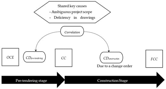
Figure 1.
Problem of the study.
This understanding will aid KSU management in making a more informed decision about continuing or stopping projects.
As previously discussed, it is necessary to technically assess the OCE, CC, and FCC’s influence on a project’s achievement. Thus, this paper first examines the correlation among OCE, CC, and FCC by performing a correlation test between the contract cost deviation of the pre-tendering stage (CDpre-tendering = (CC − OCE)/CC) and the cost deviation of construction stages (CDconstruction = (FCC − CC)/CC) for 34 projects at KSU. The correlation results indicated the relationship between CDpre-tendering and CDconstruction. This paper presents a case study based on the author’s experience that details how a lack of owner vision and need before signing a construction contract could lead to increased FCC and project risk. In addition, the main purpose of this paper is to develop a forecast model to estimate the FCC using an artificial neural network. To develop the model, the deviation costs in the two stages (pre-tendering and construction) were examined using two methods (the case study and the correlation test).
Due to the limited project data, the data were prepared using useful transformation functions. For the prediction of the FCC based on the CC and OCE, 2 linear regression models were developed on the basis of 34 projects’ data and their square-root-transformed data. Moreover, an artificial neural network (ANN) was developed. The data were standardized using Zavadskas and Turskis’ logarithmic method and applied to the ANN model. The models were evaluated using mean absolute percentage error (MAPE). The findings show that the developed ANN model assists construction parties (clients and contractors) in reasonably predicting the FCC depending on pre-tendering information (OCE and CC). The paper’s flow chart is shown in Figure 2.
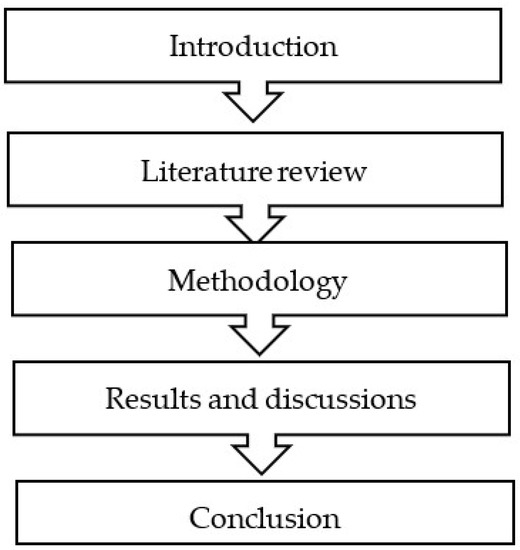
Figure 2.
Flow chart of the paper.
This study’s contributions are the provision of an ANN model for forecasting FCC on the basis of the OCE and CC value in the early stage. In addition, this study presents a data processing method to deal with relatively small input and output data and utilize the processed data for ANN, which is a valuable technique for improving the forecast model results. Moreover, this paper presents a case study showing the motive to perform this research. The case study illustrates the difference between the OCE and CC value and the increased FCC during construction, concluding with five lessons learned.
2. Literature Review
The aim of reviewing former studies is to highlight the relationship between the change in the OCE and FCC, as mentioned before. In addition, this section reviews the formally predicted models to demonstrate this study’s originality of a forecasted model that correlates with the OCE and FCC.
2.1. Factors Affecting the OCE and Bidding Deviation
During bidding time, the limited availability of information may hinder the decision-maker from signing a construction contract. Thus, several studies have attempted to facilitate the process of creating an informed decision for owners and contractors signing a contract and searching for alternatives to financing the project. Saqer et al. [10] identified various factors influencing the difference between the CC and OCE. These factors were split into three categories: external factors related to a job, environmental, and internal factors. In the State of Louisiana, USA, between 2011 and 2015, Baek et al. [11] developed a linear regression (LR) analysis method to measure the impacts of relevant factors on the bid price difference and identify factors impacting it. According to their findings, the bid price difference is significantly influenced by the bidding competition level, the scope of the contract, and the number of activities. Senouci et al. [12] studied the relationship between the CC and cost overrun for road, building, and drainage projects in Qatar using statistical analysis. They found that the cost overrun of the building project increased with the increase in the contract cost. On the basis of 74 road project data constructed in Palestine, Mahamid [13] showed that the significant impacts on the cost deviation were project size, terrain condition, and soil stability. Additionally, a review of the variables influencing OCE in building projects in different places was conducted by [9]. In most countries, they found that the three most important factors influencing OCE’s accuracy in construction projects were having a short time to prepare an estimate, inaccurate and non-reliable cost data, and sketches with ambiguous details.
On the basis of the above review, it can be concluded that the significant source factor impacting the project bidding process is a lack of information and defining the owner’s project objectives. This unclear situation affects the completion of the design drawing and the cost estimation period.
2.2. Factors Affecting Changes CC and Change Orders
Increasing the project change orders and the CC causes the owners great concern and risk. Hence, managing the cash flow and prioritizing the owner’s expenses is problematic [14]. Many researchers have studied this change order fact to understand why it happens. Khalifa and Mahamid [15] stated that the top five reasons for Saudi’s change orders include the owner’s additional work, flaws and omissions in the design, a lack of coordination between the parties involved in the construction, poor quality, and the owner’s financial issues. Elbeltagi et al. [16] determined from 384 feedback questionnaires that owner changes and poor design documents are the main reasons behind change orders.
Moreover, Alnuaimi et al. [17] determined, on the basis of case studies and a questionnaire, that the owner’s needs and design revisions in Omani projects were the most significant factors causing change orders. In India, Desai et al. [18] found that the owner’s financial problems and change of scope and design were the main factors causing change orders on the basis of 70 respondents from several categories of construction professionals using RII methods (Relative Important Index). Finally, in a UK study, Keane et al. [14] used case studies and questionnaire surveys to conclude that the most frequent change order causes are errors and omissions, ambiguous design details, poor design, and poor working drawing details.
In the previous study’s findings, the authors observed that the absence of the owner’s needs was the primary reason behind change orders in construction and the FCC.
2.3. Former Forecast Cost Construction Models
This section reviews several studies on the forecast model since 1971 in the cost construction area. Capen et al. [19] created a mathematical bidding model utilizing information from oil and gas company drilling contracts. The research revealed the following bidding guidelines: the lower companies bid, fewer competitors know, less estimate confidence, and the lower number of raised bids. Bromilow [20] developed a regression model for predicting contract duration on the basis of the estimated final cost of the construction project, and the method was based on the contract period. Skitmore and Ng [7] developed an LR model to forecast the FCC and the actual duration of the project. The LR model was based on the CC and contract duration of the project and considered contractor selection and contractual arrangement in the account.
To predict the required number of bids in the competition, Ngai et al. [21] designed a regression model. This model depended on a sample of 229 Hong Kong construction projects. The connection between the number of bids and the deviation of pre-bid estimates was established by [22]. The correlation coefficient was statistically significant.
On the basis of 927 construction projects in Utah state, the United States of America (USA), Li et al. [23] evaluated how the number of bidders affects bid prices by developing a regression model utilizing the percentage difference among the third-lowest, second-lowest, and lowest bid as the dependent variables. Li et al. [24] developed a model for forecasting the ratio of a low bid to an OCE using time series analysis and highway project data collected from the Georgia Department of Transportation, USA. In addition, Li et al. [25] recently utilized the previous data model for forecasting the ratio of a low bid to the OCE using feedforward neural networks and highway project data collected from the same transportation department in the USA.
To support the originality of our research, Table 1 represents 17 studies that introduced forecast models in different areas of construction cost and risk with different parameters, shown in the column table titles. This table reveals that none of the past studies used the CC and OCE as input for predicting the FCC.

Table 1.
Summary of methods used to determine the forecasted final contract price.
3. Case Study and Study Hypotheses
To support the main study’s claim that the causes of the change in OCE at the pre-tendering stage are similar to the causes of the change in CC at the construction stage, this section introduces a case study based on the author’s experience and previous research. This case study highlights the effect of unclear owner needs on a contract’s value. In this case study, an owner/investor decided to build a hotel on their land. The owner provided part of the fund for the hotel project budget as an investment. The owner has previous experience constructing such types of hospitality buildings with an operator. The owner signed a contract with a well-known hotel operator to enhance the hotel’s marketing and provide the standards necessary to uphold the standard of hotel service. Later, because the owners desired to open the hotel early to avoid losing the market, the owner signed a contract with a contractor with less information about the hotel’s requirements. Due to the short design period and lack of contact between the operator, owner, and designer, the project designer needed to be aware of the hotel’s necessities. Subsequently, the owner decided to award the project to a contractor with partially complete drawings to expedite the building process and capture market share by opening the hotel quickly. Thus, the project started to be affected by increased change orders, resulting in a dispute between the owner and the contractor. The owner decided to employ a mediator’s Engineering and Architecture office to evaluate the work value achieved to create a settlement between the two contract parties. The mediator reached an agreed amount of funds paid to the contractor by the owner.
Much later, the owner signed another contract with a less-complete vision of the drawing needs. The new contractor started the work; however, the project suffered from hotel operator changes due to a new hotel standard. The hotel standard changed as a result of the prolonged execution of the project. The owner and the contractor agreed to accept these changes to compete in the hotel market. Accordingly, the new contractor struggled to manage their subcontractors due to the lengthy procedure of hotel operator approval. The situation worsened as all parties suffered from increased market prices and overhead costs.
Consequently, many changes became required, and the owner managed to fund the substantial increase in CC. The FCC increased significantly in this project. The lessons learned in this case study are:
- Entering fewer complete drawings in a hotel project is a considerable risk. It is highly recommended to obtain design drawings fully approved by the hotel operator to control the project cost.
- Hotel investors must calculate the opportunity income or benefits before choosing a fixed construction contract.
- In such a hospitality project, more than traditional value engineering analysis is needed. Involved parties should also study the market’s value and competitiveness in addition to defining the project’s quality, function, and cost.
- It is recommended to control the hotel operators’ requests to increase the hotel’s quality. It is crucial that owners or investors study these requests carefully. Usually, the operator needs to maximize the hotel cost during construction to gain more profit after opening the hotel. Any expenses during the hotel operation will be reduced from project income and then minimize the hotel operator’s profit.
- Using the forecasting technique described in this study could help the owner make a more informed decision and manage project risks before accepting any commitments.
From the previous case study, it can be concluded that the lack of drawing completion increased the project’s work scope, impacting both the OCE and FCC. Thus, on the basis of the OCE and FCC similarities in shared causes, in addition to the authors’ project management expertise, we can conclude our study hypothesis. The hypothesis is that there is a strong correlation between the CC and OCE difference and the FCC and CC difference. Shrestha and Pradhananga [37] studied the correlation between the previous values; however, they did not develop a forecast model in their study on the basis of this correlation.
4. Methodology
The methodology consists of five steps: data collection (to create a database for the development of the ANN model); conducting a correlation test (to examine the relationship among CC, OCE, and FCC before developing the ANN model); carrying out a sample size and normality test (to check whether the sample represents the sample community and distribution of the data follows a normal distribution); and developing an appropriate model. The flow chart of the methodology is shown in Figure 3.
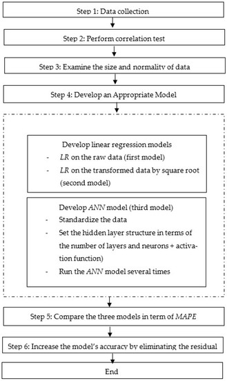
Figure 3.
Flow chart methodology.
Sample size and normality.
4.1. Step 1: Data Collection
The first stage is to collect data from the completed construction projects in Saudi Arabia, which is required to develop and validate forecasting models. The data of the cost estimation accuracy cost represent 34 projects conducted at KSU from 2011 to 2021. The projects include building, highway, electric, and mechanic projects. The data consisted of the initial OCE, CC, and FCC of 34 projects, as shown in Figure 4a–c. Figure 5 depicts the difference between FCC and CC for the 34 projects. In this figure, it can be seen that in approximately 40% (14/34) of projects, the FCC is not changed (i.e., FCC − CC = 0), while 60% of projects are changed due to new project requirements.
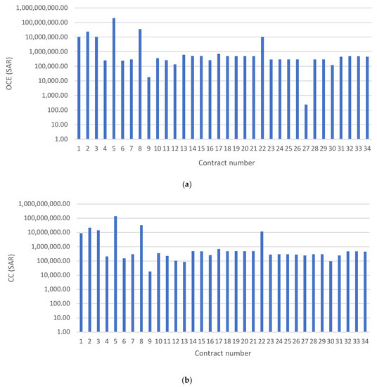
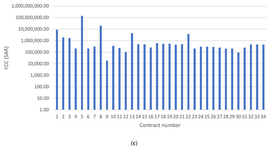
Figure 4.
The 3 costs in the 34 projects: (a) owner’s estimate cost (OCE), (b) contract cost (CC), and (c) final contract cost (FCC).
Figure 5.
Absolute difference between final contract cost (FCC) and contract cost (CC) of 34 projects.
4.2. Step 2: Perform Correlation Tests
Before data analysis and construction of reliability models, it is assumed in this study that the two critical causes of OCE at the early stage of the project will be continued over the construction phase and cause changes to CC to reach FCC. The relationship among the different costs was examined by studying the cost deviation of the pre-tendering and construction phases. These two cost deviations can be computed using Equations (1) and (2), respectively.
4.3. Step 3: Examine the Size and Normality Tests of the Data
As the sample space (construction projects) is large and unknown, the sample size can be computed using Equation (3):
where Z is a value corresponding to a 95% confidence level and is equal to 1.96, and p represents the probability choice, which is 0.5. C is the confidence interval, which should be less than 0.2 [26].
4.4. Step 4: Develop an Appropriate Model
Due to limited data collection, the independent variables, such as the OCE and CC, may not be correlated with the dependent variable, the FCC. Hence, different models were developed and assessed. The models utilized were the linear regression model for the raw data, the linear regression model for the transformed data by square root, and the ANN model. The raw data were treated for the second and third models. For the second model, the data were transformed by taking square roots for input and output data. In addition, the output computed by the second model was untransformed by taking the squares to evaluate the model.
The ANN model is a model that estimates the output by learning an algorithm from an arbitrary function [38]. The general structure of the ANN model consists of the input, hidden, and output layers, as shown later in the final ANN structure model in this study. The hidden layer may have one or multiple layers with numbers of neurons, while the number of neurons at the input and output layer depends on the purpose of the model. In a typical ANN, the neurons of the input layer generally connect to each neuron at the hidden layer. Then, each neuron at the hidden layers connects to neurons of the output layer. Each connector has weight and bias values. The mathematical equation capturing weights and bias among neurons in the three layers in ANN is expressed for one and two hidden layers in Equations (4) and (5), respectively, as
where Yoi is output variable i, is the activation function of the output layer, is output layer bias, is a connection weight between the jth hidden neuron at the second hidden layer and single output neuron, is the activation function of the second hidden layer and single output neuron, is activation function of the first hidden layer, is a bias of the jth hidden layer (second hidden layer; j = 1, …, J), is a bias of the kth hidden neuron (first hidden layer; k = 1, …, K), is connection weight between the kth hidden neuron (at first hidden layer) and jth hidden neuron (at second hidden layer), and is connection weight between i input variables (i = 1, …, N) and the kth hidden neuron. is the i input variable.
In terms of activation function, the hyperbolic tangent and sigmoid function are represented in Equations (6) and (7), respectively, as
The data were from 34 projects and were small in number. However, ANN requires extensive data to create a reliable model. Several studies used different techniques to increase the precision of the ANN model and overcome the limited data issues, as shown in Table 2. This paper used the 3 techniques to handle 34 projects’ data in an ANN. We standardized the OCE, CC, and FCC by an appropriate method followed by [39]; ran the ANN model several times to avoid the overfitting issue as mentioned by [40]; and eliminated data that had residual error, as expressed by [41]. It is worth noting that the correlation analysis techniques were excluded from the paper due to the limited predictors (OCE and CC).
Table 2.
Literature aimed at improving neural network performance to handle relatively little data.
Several standardized methods were used for the input and output data of ANN. Anysz et al. [40] summarized the five standardized methods as vector standardization, Manhattan standardization, maximum linear standardization, Weitendorf’s linear standardization, Peldschus’ nonlinear standardization, and Zavadskas and Turskis’ logarithmic standardization. They concluded that Zavadskas and Turskis’ logarithmic standardization method provided the minimum errors. Therefore, it was utilized as a standardized method in this paper. The input (Ni) and output data (Oi) were standardized as follows:
where and are standardized using the input and output values, respectively; n is the number of data points. The number of hidden neurons is recommended as (2m + 1), where m is the number of input layer neurons [43]. Due to the m being 2, the number of neurons per each hidden layer was 5. Moreover, the type of activation function used in this paper was a hyperbolic function, and the number of hidden layers was two.
The data used in the ANN model were divided into training data (70%) and testing data (30%). Then, the model was evaluated by measuring the relative error (RE) for the training and testing process. It should be noted that the two data types were arbitrarily selected among all data. To obtain a homogenous distribution of the training and testing data, the ANN model was run three times, which was generally based on the testing data percentage. Then, the RE was examined in training and testing groups each time.
The output of the ANN model should be reversed, and we should obtain the estimated output value (estimated FCC) to assess the model using MAPE value, as mentioned in the following section. To obtain the , the ANN in the SPSS program provides . Due to the ANN being run three times, the had three values, and their average was computed . On the basis of Equation (9), the was computed after setting as and setting as . Figure 6 represents the ANN structure used in this paper.
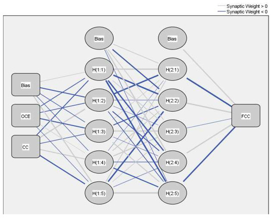
Figure 6.
The ANN structure.
4.5. Step 5: Assessment and Evaluation Models
The three models were evaluated using mean absolute percentage errors (MAPE) on the basis of the estimated output () and observed output (), as computed in Equation (10).
where is the estimated value (FCC) computed by the three models after considering the untransformed square root for the second model and the reverse value for the third model (ANN model). The model that has the smallest MAPE value is the appropriate model.
4.6. Step 6: Increase the Model’s Accuracy
If the three MAPE values are unsatisfactory (MAPE is greater than 25%), the model with the lowest value increases its accuracy. This technique ensures the normalization of data, makes training less sensitive, and increases the ANN model. The absolute percentage error of each observation (APE) that was based on the estimated output () and observed output () was used to evaluate the eliminate the abnormal data. This can be computed using Equation (11).
The cases with APE values greater than 35% were deleted from the data.
5. Results and Discussion
5.1. Results of Correlation, Sample Size, and Normality Tests
The resulting correlation test is shown in Table 3; the Pearson correlation and p-value were −0.968 and less than 0.001, respectively. The correlation coefficient shows a highly negative correlation, where the overestimated cost deviation in pre-tendering leads to underestimated cost deviation in the construction phase.
Table 3.
Correlation test results.
In terms of the sample size and normality test, the C value, as shown in Equation (3), was 0.17, which is less than 0.2. Regarding the normality test, the collected data should follow a normal distribution. Hence, a normality test for collected data with their transformation should be conducted. Table 4 shows the results of the normality test. The p-values of the Kolmogorov–Smirnov and Shapiro–Wilk tests were less than 0.05 for all data, as shown in Table 3. Therefore, the OCE, CC, and FCC followed a normal distribution.
Table 4.
Normality test of transformed data.
5.2. ANN Model
The linear equation regression for the first model (LR on the raw data; 34 data sets) and the second model (LR on the transformed data by square root) is shown in Equations (12) and (13).
The two models refer to the OCE leading to an increase in the FCC. However, the CC leads to a decrease in FCC. In terms of the ANN model, after standardized the data using Zavadskas and Turskis’ logarithmic method, the REs of the training and testing data are shown in Table 5. The RE for the training stage is smaller than that for the testing stage. This is due to the limited data used in the testing stage and generates a high error. Moreover, the RE of the testing stage was higher than the value recommended by [6]. This issue is addressed later.
Table 5.
Relative errors of the ANN model for the three runs.
To evaluate the three models, the MAPE of Model 1 was 125.27%. Its value is low for the second model, 66.89%, reduced by 58.38%. In addition, the MAPE value of the ANN model (third model) was 45.27%, smaller than the first and the second model by 80.05% and 21.67%, respectively. The decreasing MAPE among the three models is because Zavadskas and Turskis’ logarithmic standardized method minimizes the raw data more than the square root function. Low-valued data are usually more oriented than higher-valued data. Thus, developing a regression model on the basis of low-valued data reduces the error values and increases the value of the determination coefficient. To enhance the above interpretation, the activation function used in the ANN model aims to reduce the input data values. For example, the input data values of Model 9 were minimized in two stages using two hidden layers, consequently producing better results than the logarithmic regression model. On the other hand, Swanson [44] stated that the model with a MAPE value larger than 25% had low accuracy and was not an acceptable prediction model. Therefore, the three models were non-acceptable models for predicting the FCC.
To increase the accuracy of the ANN model (third model), which provided the smallest MAPE value compared with the first and the second model, the data with high residual errors were eliminated. This method was carried out by [41,43].
The 12 projects (cases) were deleted, and the cases with an APE value smaller than or equal to 35% was 22, as shown in Table 6.
Table 6.
The twenty-two data sets after eliminating the APE values greater than 35%.
The twenty-two data sets were utilized to develop the ANN model using Zavadskas and Turskis’ logarithmic standardized method. The results of the training and testing accuracy of the ANN model that was carried out three times are shown in Table 7. The minimum and maximum relative errors of the training and testing accuracy were 0.004 and 0.112, respectively, and less than 0.2.
Table 7.
Relative errors of the ANN model with the twenty-two data sets after three runs.
The MAPE value was 8.74%, indicating high accuracy in the evaluation of the ANN model based on the twenty-two data sets. It was 36.48% smaller than the ANN based on the thirty-four data sets. Moreover, the MAPE of the developed ANN model by Badawy [6] was 10.98, slightly higher than the ANN model. The frequencies of the percentage error are illustrated in Figure 7. The APE’s mean, maximum, and minimum were 1.46%, 85%, and 0.4%, respectively. The mean and the standard deviation were 0.52% and 0.755%, respectively. Moreover, the APE of 18 of the 22 data sets was less than 0.5%, while 3 had an APE of less than 1.0%.
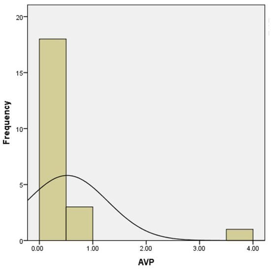
Figure 7.
Frequency of APE of the ANN model.
The relationship between the estimated FCC computed by the ANN model (on the horizontal axis) and the observed FCC (on the vertical axis) is depicted in Figure 8. The determination coefficient (R2) of the trend line was 0.965, which indicates that there is a robust correlation between the estimated and observed FCC, and it is close to the best value (1.0) [45].
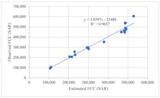
Figure 8.
Correlation between estimated FCC and observed FCC.
To compare the result of this study with previous ones in terms of overall results, this study demonstrated a relationship between the cost deviation in the pre-tendering stage (CC and OCE) and the construction stage (FCC and CC). This finding agrees with the result of a correlation study [6]. In addition, Skitmore and Ng [7] and Aretoulis [8] confirmed the role of CC in predicting FCC, which agrees with this study.
Moreover, the limited data significantly hindered forecasting analysis in prior studies, especially in ANNs. To overcome the limited data issue, this study applied different transformed functions in ANN models, which have not been achieved in previous studies related to contracting costs. Skitmore and Ng [7] processed construction cost data before application in the LR; however, this method has not previously been used in an ANN. Badawy [6] utilized ANN construction cost analysis without data processing for contracts. Finally, decision-makers can use this valuable projected model to forecast how to manage their budgets and FCC risk.
6. Recommendation and Future Study
The authors recommend expanding this study with large amounts of data from different parts of the world. Furthermore, the authors suggested incorporating this paper’s results into system dynamics to capture the dynamic effect of the various factors on the change in FCC.
7. Conclusions
A set of 34 projects from KSU was utilized to establish an ANN to forecast the FCC after performing correlation, sample size, and normality tests. Due to the limited number of projects, the data were prepared by applying standardization using Zavadskas and Turskis’ logarithmic method for dependent and independent variables (FCC, OCE, and CC). Two hidden layers with five neurons per layer were used, and the activation function was hyperbolic. The ANN model was run three times to ensure that the training and testing sets were evenly distributed among the data. After that, the ANN model’s results were compared with the LR models developed on the basis of the raw data (the first model) and the square-root-transformed data (the second model) using MAPE. The findings revealed that the ANN model had a MAPE value smaller than the two LRs (first and second models). However, the accuracy of the ANN model was low, with a MAPE value of more than 45%. Therefore, elimination of data with an APE of greater than 35% was implemented, and the remainder were integrated into the ANN model. The model’s accuracy was enhanced by decreasing its MAPE value to 8.7%. The information in this paper assists decision-makers in deciding whether to continue to fund a project, discontinue it, or consider other risk management alternatives.
Author Contributions
Conceptualization, A.M.A. and K.S.A.-G.; data curation, N.M.A.; formal analysis; N.M.A. and K.S.A.-G.; funding acquisition, A.M.A. and K.S.A.-G.; investigation, A.M.A., N.M.A., and K.S.A.-G.; methodology, N.M.A. and K.S.A.-G.; project administration, A.M.A. and K.S.A.-G.; resources, A.M.A. and K.S.A.-G.; software, N.M.A.; supervision, A.M.A. and K.S.A.-G.; validation, N.M.A. and K.S.A.-G.; visualization, A.M.A., N.M.A., and K.S.A.-G.; roles/writing—original draft, A.M.A., N.M.A., and K.S.A.-G.; writing—review and editing, A.M.A., N.M.A., and K.S.A.-G. All authors have read and agreed to the published version of the manuscript.
Funding
The authors extend their appreciation to the Deputyship for Research & Innovation, Ministry of Education in Saudi Arabia for funding this research work through the project no. (IFKSURG-2- IFKSURG-2).
Data Availability Statement
The raw data supporting the findings of this paper are available upon request from the corresponding author.
Acknowledgments
The authors would like to thank the King Saud University (KSU)-Project Administrative for providing the data for this research.
Conflicts of Interest
The authors declare no conflict of interest.
References
- Christensen, D.S.; Gordon, J.A. Does a Rubber Baseline Guarantee Cost Overruns on Defense Acquisition Contracts? Proj. Manag. J. 1998, 29, 43–51. [Google Scholar] [CrossRef]
- Thomas, N.; Thomas, A.V. Regression Modelling for Prediction of Construction Cost and Duration. Appl. Mech. Mater. 2016, 857, 195–199. [Google Scholar] [CrossRef]
- Gao, X.; Pishdad-Bozorgi, P. A framework of developing machine learning models for facility life-cycle cost analysis. Build. Res. Inf. 2020, 48, 501–525. [Google Scholar] [CrossRef]
- Ye, D. An Algorithm for Construction Project Cost Forecast Based on Particle Swarm Optimization-Guided BP Neural Network. Sci. Program. 2021, 2021, 4309495. [Google Scholar] [CrossRef]
- Lowe, D.J. Predicting construction cost using multiple regression techniques. J. Constr. Eng. Manag. 2006, 132, 750–758. [Google Scholar] [CrossRef]
- Badawy, M. A hybrid approach for a cost estimate of residential buildings in Egypt at the early stage. Asian J. Civ. Eng. 2020, 21, 763–774. [Google Scholar] [CrossRef]
- Skitmore, R.M.; Ng, S.T. Forecast models for actual construction time and cost. Build. Environ. 2003, 38, 1075–1083. [Google Scholar] [CrossRef]
- Aretoulis, G.N. Neural network models for actual cost prediction in Greek public highway projects. Int. J. Proj. Organ. Manag. 2019, 11, 41. [Google Scholar] [CrossRef]
- Albtoush, F.; Ing, D.S.; Rahman, R.A.; Al-Btoosh, J.A.A. Factors Affecting the Accuracy of Cost Estimate in Construction Projects: A Review. In Proceedings of the National Conference for Postgraduate Research (NCON-PGR 2020), Virtual Mode, 9 December 2020; pp. 1–9. [Google Scholar]
- Saqer, F. Development of Cost Estimation Model for Ministry of Youth and Sports Affairs Construction Projects A Case study from Kingdom of Bahrain. Master’s Thesis, University of Bahrain, Manama, Kingdom of Bahrain, 2020. [Google Scholar]
- Baek, M.; Ashuri, B. Assessing low bid deviation from engineer’s estimate in highway construction projects. In Proceedings of the 55th Associated Schools of Construction Annual International Conference, Denver, CO, USA, 10–13 April 2019; pp. 371–377. [Google Scholar]
- Senouci, A.; Ismail, A.; Eldin, N. Time Delay and Cost Overrun in Qatari Public Construction Projects. Procedia Eng. 2016, 164, 368–375. [Google Scholar] [CrossRef]
- Mahamid, I. Contractors’ perception of risk factors affecting cost overrun in building projects in Palestine. IES J. Part A Civ. Struct. Eng. 2014, 7, 38–50. [Google Scholar] [CrossRef]
- Keane, P.; Sertyesilisik, B.; Ross, A.D. Variations and Change Orders on Construction Projects. J. Leg. Aff. Disput. Resolut. Eng. Constr. 2010, 2, 89–96. [Google Scholar] [CrossRef]
- Khalifa, W.M.A.; Mahamid, I. Causes of Change Orders in Construction Projects. Eng. Technol. Appl. Sci. Res. 2019, 9, 4956–4961. [Google Scholar] [CrossRef]
- Elbeltagi, E.; Elshahat, A.; Dawood, M.; Alaryan, A. Causes and Effects of Change Orders on Construction Projects in Kuwait. Int. J. Eng. Res. Appl. 2014, 4, 1–8. [Google Scholar]
- Alnuaimi, A.S.; Taha, R.A.; Al Mohsin, M.; Al-Harthi, A.S. Causes, Effects, Benefits, and Remedies of Change Orders on Public Construction Projects in Oman. J. Constr. Eng. Manag. 2010, 136, 615–622. [Google Scholar] [CrossRef]
- Desai, J.N.; Pitroda, J.; Bhavasar, J.J. Analysis of Factor Affecting Change Order in Construction Industry Using RII Method. Int. J. Mod. Trends Eng. Res. 2015, 2, 344–347. [Google Scholar]
- Capen, E.C.; Clapp, R.V.; Campbell, W.M. Competitive bidding in high-risk situations. J. Pet. Technol. 1971, 23, 641–653. [Google Scholar] [CrossRef]
- Bromilow, F.J. Measurement and scheduling of construction time and cost performance in the building industry. Chart. Build. 1974, 10, 57–65. [Google Scholar]
- Ngai, S.C.; Drew, D.S.; Lo, H.P.; Skitmore, M. A theoretical framework for determining the minimum number of bidders in construction bidding competitions. Constr. Manag. Econ. 2002, 20, 473–482. [Google Scholar] [CrossRef]
- Carr, P.G. Investigation of bid price competition measured through prebid project estimates, actual bid prices, and number of bidders. J. Constr. Eng. Manag. 2005, 131, 1165–1172. [Google Scholar] [CrossRef]
- Li, S.; Foulger, J.R.; Philips, P.W. Analysis of the impacts of the number of bidders upon bid values: Implications for contractor prequalification and project timing and bundling. Public Work. Manag. Policy 2008, 12, 503–514. [Google Scholar]
- Li, M.; Baek, M.; Ashuri, B. Forecasting Ratio of Low Bid to Owner’s Estimate for Highway Construction. J. Constr. Eng. Manag. 2021, 147, 04020157. [Google Scholar] [CrossRef]
- Li, M.; Zheng, Q.; Ashuri, B. Predicting Ratio of Low Bid to Owner’s Estimate Using Feedforward Neural Networks for Highway Construction. In Proceedings of the Construction Research Congress, Arlington, VA, USA, 9–12 March 2022; pp. 340–350. [Google Scholar]
- Badawy, M.; Alqahtani, F.; Hafez, H. Identifying the risk factors affecting the overall cost risk in residential projects at the early stage. Ain Shams Eng. J. 2022, 13, 101586. [Google Scholar] [CrossRef]
- Ngo, K.A.; Lucko, G.; Ballesteros-Pérez, P. Continuous earned value management with singularity functions for comprehensive project performance tracking and forecasting. Autom. Constr. 2022, 143, 104583. [Google Scholar] [CrossRef]
- Leon, H.; Osman, H.; Georgy, M.; Elsaid, M. System Dynamics Approach for Forecasting Performance of Construction Projects. J. Manag. Eng. 2018, 34. [Google Scholar] [CrossRef]
- Natarajan, A. Reference Class Forecasting and Machine Learning for Improved Offshore Oil and Gas Megaproject Planning: Methods and Application. Proj. Manag. J. 2022, 53, 456–484. [Google Scholar] [CrossRef]
- Espinosa-Garza, G.; Loera-Hernández, I. Proposed model to improve the forecast of the planned value in the estimation of the final cost of the construction projects. Procedia Manuf. 2017, 13, 1011–1018. [Google Scholar] [CrossRef]
- Odeyinka, H.; Lowe, J.; Kaka, A. Regression modelling of risk impacts on construction cost flow forecast. J. Financ. Manag. Prop. Constr. 2012, 17, 203–221. [Google Scholar] [CrossRef]
- Xu, C.; Wang, Y.; Ye, K.; Zhang, S.; Zou, M.; Chen, C. Research on transmission line project cost forecast method based on BP neural network. IOP Conf. Ser. Mater. Sci. Eng. 2019, 688, 055074. [Google Scholar] [CrossRef]
- Ng, S.T.; Cheung, S.O.; Skitmore, M.; Wong, T.C.Y. An integrated regression analysis and time series model for construction tender price index forecasting. Constr. Manag. Econ. 2004, 22, 483–493. [Google Scholar] [CrossRef]
- Kim, B.-C.; Reinschmidt, K.F. Combination of Project Cost Forecasts in Earned Value Management. J. Constr. Eng. Manag. 2011, 137, 958–966. [Google Scholar] [CrossRef]
- Mir, M.; Kabir, H.D.; Nasirzadeh, F.; Khosravi, A. Neural network-based interval forecasting of construction material prices. J. Build. Eng. 2021, 39, 102288. [Google Scholar] [CrossRef]
- Moghayedi, A.; Windapo, A. Predicting the impact size of uncertainty events on construction cost and time of highway projects using ANFIS technique. In Collaboration and Integration in Construction, Engineering, Management and Technology; Springer: Berlin/Heidelberg, Germany, 2021; pp. 203–209. [Google Scholar]
- Shrestha, P.P.; Pradhananga, N. Correlating bid price with the number of bidders and final construction cost of public street projects. Transp. Res. Rec. 2010, 2151, 3–10. [Google Scholar] [CrossRef]
- Loy, J. Neural Network Projects with Python: The Ultimate Guide to Using Python to Explore the True Power of Neural Networks Through Six Projects; Packt Publishing: Birmingham, UK, 2019. [Google Scholar]
- Anysz, H.; Zbiciak, A.; Ibadov, N. The Influence of Input Data Standardization Method on Prediction Accuracy of Artificial Neural Networks. Procedia Eng. 2016, 153, 66–70. [Google Scholar] [CrossRef]
- Pasini, A. Artificial neural networks for small dataset analysis. J. Thorac. Deisease 2015, 7, 953–960. [Google Scholar]
- Zayed, T. Assessment of Productivity for Concrete Bored Pile Construction. Ph.D. Dissertation, Purdue University, West Lafayette, IN, USA, 2001. [Google Scholar]
- Amiri, A.; Mirzakuchaki, S. A digital watermarking method based on NSCT transform and hybrid evolutionary algorithms with neural networks. SN Appl. Sci. 2020, 2, 1669. [Google Scholar] [CrossRef]
- Vinayagam, R.; Dave, N.; Varadavenkatesan, T.; Rajamohan, N.; Sillanpää, M.; Nadda, A.K.; Govarthanan, M.; Selvaraj, R. Artificial neural network and statistical modelling of biosorptive removal of hexavalent chromium using macroalgal spent biomass. Chemosphere 2022, 296, 133965. [Google Scholar] [CrossRef]
- Swanson, D.A. On the Relationship among Values of the Same Summary Measure of Error when It Is Used across Multiple Characteristics at the Same Point in Time: An Examination of MALPE and MAPE1. 2015. Available online: https://escholarship.org/content/qt1f71t3x9/qt1f71t3x9_noSplash_9c507cef1229a954e3e9b7a2ee9ef217.pdf?t=o5wul1 (accessed on 15 March 2023).
- Chicco, D.; Warrens, M.J.; Giuseppe, J. The coefficient of determination R-squared is more informative than SMAPE, MAE, MAPE, MSE and RMSE in regression analysis evaluation. PeerJ Comput. Sci. 2021, 7, e623. [Google Scholar] [CrossRef]


Disclaimer/Publisher’s Note: The statements, opinions and data contained in all publications are solely those of the individual author(s) and contributor(s) and not of MDPI and/or the editor(s). MDPI and/or the editor(s) disclaim responsibility for any injury to people or property resulting from any ideas, methods, instructions or products referred to in the content. |
© 2023 by the authors. Licensee MDPI, Basel, Switzerland. This article is an open access article distributed under the terms and conditions of the Creative Commons Attribution (CC BY) license (https://creativecommons.org/licenses/by/4.0/).