Abstract
Self-tapping screws (STS) are used in wood-to-wood and wood-to-steel connections in timber structures. Premature failure of STS during the construction phase has been reported by structural engineers and contractors in relation to a few North American mass-timber projects. This STS failure type is suspected of having been precipitated by additional axial stress exerted on STS from swelling of the wood resulting from prolonged wetting. This study investigates the axial stress distribution of STS installed in two mass timber products, cross-laminated timber (CLT) and glulam, under axial loading and changing moisture conditions in the linear elastic regime. The focus is on modelling the stress distribution of STS during wood-wetting. Properties of self-tapping screws under axial loads, such as tensile and withdrawal properties, along with swelling properties of CLT and glulam, have been investigated. A numerical method to predict the axial stress distribution of the screw from these material property tests has been developed. The numerical model has been calibrated with test results. The method developed in this research helps in understanding the premature failure of self-tapping screw connections under the moisture content variation of wood. The next step will be developing an analytical model to predict the axial stress distribution of STS.
1. Introduction
Mass-timber construction is making headway in the construction industry of North America. Self-tapping screws (STS) have become very popular for use in mass-timber products (e.g., cross-laminated timber, glulam, nail-laminated timber, etc.) due to their easier installation, stiffer resulting connections, and availability in large lengths and diameters [1]. STS are preferably used in wood members at an angle to the grain direction of the main wood member. Recently the load-carrying capacity of screws in tension (load acting along the screw axis) has been a focus compared to the lateral load-carrying capacity of the screw (load acting perpendicular to the screw axis). When the screw is subjected to a tension load, the condition can be considered the axial loading condition of the screw. In steel-to-wood and wood-to-wood member connections of mass timber structures, the axial behaviour of screws is pivotal for correctly predicting their performance.
In North America, premature tensile failure of self-tapping screws has been noted during construction. The induced axial load in the screw from the torquing action, coupled with the additional axial force exerted on the screw from moisture swelling of the surrounding wood, is suspected of causing the premature tensile failure of the self-tapping screw.
The axial stress distribution in dowels [2] and self-tapping screws [2,3,4] due to axial load has been investigated in previous studies. However, the axial stress distribution in a self-tapping screw under the simultaneous action of axial loading and moisture swelling of wood has not been investigated. Understanding the axial stress distribution in a self-tapping screw under the simultaneous action of axial loading and moisture swelling of wood is critical to developing solutions to address the problem related to the noted premature tensile failure mechanism of self-tapping screws.
Wood is a hygroscopic material, and mass timber products undergo hygroscopic deformation due to the wood’s moisture content variation. The hygroscopic deformation arising from the moisture content increase of wood causes an increase in the volume called moisture swelling. Hygroscopic deformation arising from the moisture content decrease in wood causes moisture shrinkage or a reduction in the volume of wood. The axial performance of STS inserted into mass timber products is affected by the additional axial stress exerted on the STS from hygroscopic deformation of the wood. The axial stress arising in STS from a combination of hygroscopic deformation of the wood and axial loading might be critical if the total maximum axial stress is close to the tensile strength of the screw. Such a situation might arise if the STS is installed in an over-torqued condition that is more than required, and the moisture content of the mass timber changes from the time of STS installation over the service life of the STS.
Attention is drawn to the case of STS inserted into wood members made of mass timber products such as glulam and CLT (cross-laminated timber), compared to wood members made of traditional timber in this study. Previous research has shown that volume changes due to moisture absorption or release under restricted movement due to the glue lines of glulam and CLT give rise to higher internal stresses than found in traditional timber [5,6]. The axial stress distribution of STS in the linear elastic regime, under the simultaneous action of axial loading and hygroscopic deformation of glulam and CLT, is numerically predicted using finite element analysis (FEA) in this research. Focus is given in this study to model the stress distribution of STS during wood-wetting (moisture swelling) as accurately as possible. The input parameters for the FEA were obtained from material property tests conducted on STS, mass timber products, and STS-mass timber composite systems. This research is the first attempt at investigating the axial stress arising in STS under the simultaneous action of hygroscopic deformation of the wood and axial loading of STS. This research used two types of mass timber products: CLT and glulam.
2. Materials and Methods
In this study, the axial stress distribution in STS inserted perpendicular to the face of mass timber members (CLT and glulam) under varying moisture conditions are numerically modelled. The specimen configurations shown in Figure 1 and moisture content changes shown in Table 1 are numerically modelled using the commercial ABAQUS FEA software [7]. As seen in Figure 1, screws of nominal outer diameters of 8 mm and 13 mm were inserted into the broad face of CLT and glulam of different sizes. The test program included two mass timber products. There was glulam made from douglas fir-larch of stress grade 16c-E and spruce-pine-fir (SPF) CLT of stress grade V2 [8]. The initial moisture condition shown in Table 1 represents the moisture content of the CLT or glulam during STS installation, and the final moisture content represents the moisture condition of the CLT or glulam due to variations in the surrounding environment. For the sake of simplicity, this study considered uniform moisture content throughout the CLT or glulam in both the initial and final stages, that is, the influence of moisture gradient was ignored. This research investigated the stress distribution of the STS in the linear elastic regime. The elastic material properties were determined from a series of tests conducted on the STS, CLT, and glulam.
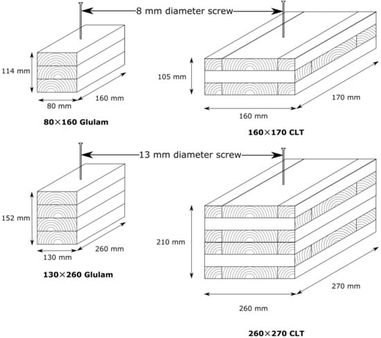
Figure 1.
CLT and glulam configurations with 8 mm screw (top row) and 13 mm screw (bottom row).

Table 1.
Finite element model configurations and moisture content changes.
2.1. Tensile Test of Self-Tapping Screws
The STS of two diameters, 8 mm and 13 mm, were tested under uniaxial tension. The average Young’s modulus, yield strength, ultimate tensile strength, strain at failure, and strain at ultimate tensile strength were determined from these tests. However, only the average Young’s modulus of the screws was used in the finite element (FE) analysis since that was the only property required for linear elastic analysis by the FE model, in addition to Poisson’s ratio. The other screw properties can be used in future research to encapsulate the behavior of the screws in the post-elastic regime.
The screw configurations shown in Table 2 were tested. The thread diameter in Table 2 is the outer thread diameter of the screw, and the root diameter is the diameter of the inner core of the screw. The number of samples tested for each screw configuration is also stated in the table. More samples were tested for screw type B, which produced a less consistent load-deformation graph. In regard to screw type B, all the screws supplied by the manufacturer were tested.
Table 2.
Screw configurations tested.
The complete tension test setup with a specimen fitted inside the test fixture is shown in Figure 2. The elongation of the screw was recorded with an extensometer attached to the thread of the screw. The applied load was measured by the load cell of the machine head. The ASTM standard E8/E8M-22 was followed for conducting the tensile tests [9].
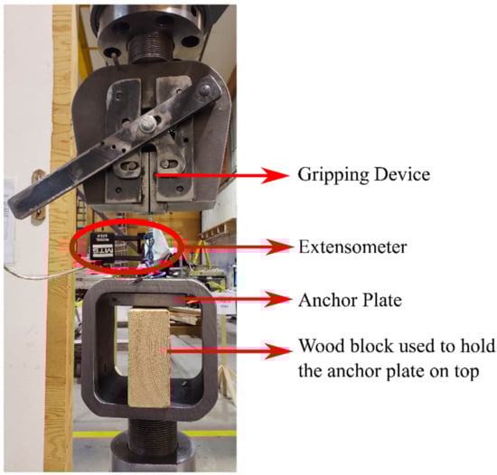
Figure 2.
Complete screw tensile test setup.
The load-elongation curves were recorded at approximately three data points per second and converted to stress–strain curves. The load at each data point was divided by the initial cross-sectional area of the core, excluding the threads, of the screw to calculate the stress. The change in length at each data point was divided by the gauge length over which the elongation was measured to determine the strain. Young’s modulus was determined by finding the slope of the fitted line of the initial linear portion of the stress–strain curve according to ASTM E111-17 [10].
2.2. Swelling Test of CLT and Glulam
The swelling behavior of the CLT and glulam products mentioned in Table 1 were investigated. The swelling coefficient of the individual laminates of the CLT and glulam was determined from the swelling strain versus moisture content change response. These swelling coefficient values were used as finite element model input for the different layers of the CLT and glulam.
Glulam of two different sizes from the same manufacturer and CLT made from 2 × 4 laminates (160 × 170 CLT) and 2 × 6 laminates (260 × 270 CLT) from two different manufacturers were tested. The two sizes of glulam and the two types of CLT used are shown in Figure 3. According to the technical specifications of the CLT manufacturer, the longitudinal (major) and the transverse (minor) layers of CLT were made from lumber of different grades. Thus, the laminates of the longitudinal and transverse layers might have come from different sources, and the swelling properties of the longitudinal and the transverse layers of CLT were determined separately. Both sizes of glulam used in the test program were of the same grade and from the same manufacturer. Furthermore, the glulam was of compression grade, which means all the laminates were of the same grade. Thus, all the layers of both sizes of glulam were considered to have the same swelling properties.

Figure 3.
CLT and glulam products used in the test program.
Small-size samples of approximate dimensions of 80 (longitudinal) mm × 35 (radial) mm × 35 (tangential) mm were cut from the different layers of CLT and glulam. It was ensured that the samples had no glue on any face. Three sample groups were prepared with these small-sized samples to investigate the dimensional changes with moisture content change. The number and type of specimens in each sample group are summarized in Table 3.
Table 3.
Specimens included in each sample group.
In two stages, each sample group was conditioned under constant relative humidity and temperature conditions. The conditioning time for each stage was two weeks. The samples were kept in a conditioning chamber in the first stage with 65 ± 2% relative humidity and a temperature of 20 °C. In the second stage, the samples were kept in another conditioning chamber. The three sample groups were kept in three different conditioning chambers in the second stage, as shown in Table 4. The first conditioning stage was adopted to achieve an equilibrium moisture content (EMC) of 12% for all specimens. The second conditioning stage aimed to achieve EMCs of 6%, 16%, and 21% (Table 4). All the samples reached a constant weight at the end of the two-week conditioning process, indicating uniform moisture content distribution inside the samples. After the two-stage conditioning, the samples were oven dried at 105 ± 1 °C for two days to achieve an oven-dry condition. The sample preparation, conditioning, and oven-drying process for the swelling tests are summarized in the flow chart shown in Figure 4.
Table 4.
Relative humidity and temperature for conditioning and the corresponding equilibrium moisture content (EMC).

Figure 4.
Flow chart of the swelling tests.
A total of nine length measurements from each sample, three along each orthotropic direction, were taken (Figure 5). Each sample’s length and weight measurements were taken at the end of the second-stage conditioning and after oven drying. A digital balance with a precision of 0.01 g was used to measure sample weight, and a digital calliper with a precision of 0.01 mm was used to measure sample dimensions. The length measurements were later used to determine the swelling strains according to Equation (1). The actual moisture content of each sample was determined using Equation (2).
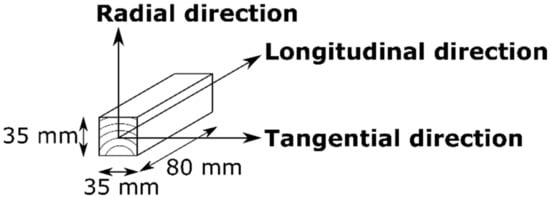
Figure 5.
Wood anatomical directions of each specimen.
The swelling coefficient can be determined by determining the slope of the swelling strain versus moisture content change graph. For this purpose, the strain values along the three orthotropic directions were recorded under different known moisture content changes. The strain value and the moisture content change of a sample can be determined using Equations (1) and (2) [6]:
where and are the oven-dry length and weight of the sample, respectively. Where and are the length and weight at the end of the second conditioning stage of the sample, is the generated swelling strain, and is the moisture content.
2.3. Withdrawal Test of Self-Tapping Screws in CLT and Glulam
Withdrawal tests were conducted on the identical specimens modelled in ABAQUS, as shown in Figure 1. The STS of the two diameters, 8 mm and 13 mm, were inserted centrically in the CLT and glulam products at a 10 d (d is the outer nominal diameter of the screw) penetration length perpendicular to the face of the specimen. The specimens were conditioned in two stages. The two-stage conditioning was performed chronologically: to achieve the initial target equilibrium moisture content (EMC) before—screw installation—conditioning to reach the final target EMC. The two-stage conditioning process was adopted to simulate the condition that the moisture content of timber members might change after screw installation in practical settings. After achieving the final target EMC, the specimens were tested in displacement control under pull–push loading conditions. The five conditioning settings adopted for the withdrawal test specimens are shown in Table 5. All the wood products and self-tapping screw combinations in the leftmost column of Table 5 were conditioned under the five conditioning settings.
Table 5.
Different specimen groups and their conditioning EMCs in the two stages used in the finite element model.
The test setup with a trial sample used for the withdrawal test is exhibited in Figure 6. The withdrawal displacement of the screw from the top wood surface was measured with two displacement (linear variable differential transformer (LVDT)) transducers. The load-displacement curve for each specimen was recorded, from which the withdrawal strength and stiffness were determined. The load-displacement curves and withdrawal test data from the withdrawal tests were used in the finite element model as input parameters.
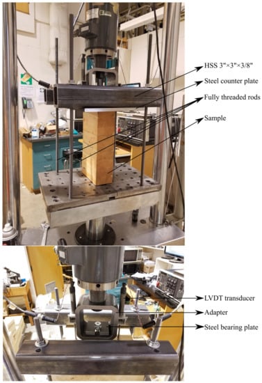
Figure 6.
Withdrawal test setup with a trial sample.
The withdrawal tests were performed to reach the maximum load within 90 ± 30 s according to the standard BS EN 1382-2016 [11]. The withdrawal strength of each screw was calculated using the following equation [12]:
Here, is the maximum applied load as measured by the machine head in N, is the outer thread diameter of the screw in mm, is the effective penetration length of the screw inside the specimen in millimeters. The effective penetration length of the screw excludes the length of the tip of the screw, which is not fully effective in imparting withdrawal resistance. The effective penetration length was determined according to the screw manufacturer’s guide.
The withdrawal displacement () of the screw is calculated using Equations (4) and (5) [12]. In Equation (4), the elongation of the free part of the screw is subtracted from the transducer measurements to get the actual value of the withdrawal displacement of the screw inside the wood:
where are the displacements recorded by the displacement transducers, is the length of screw protrusion outside the CLT or glulam in millimeters, is Young’s modulus of the material of the screw in MPa, is the applied load at each data point in N, defined in Equation (5) is the tensile stress in the screw in MP, and is the inner core diameter of the screw in millimeters. The inner core diameter of the screw has been used here based on the premise that the screw core provides the axial rigidity of the protruded part of the screw. The effective length, based on the screw manufacturers’ guide, and the length of screw protrusion for the different screws used in the test program are mentioned in Table 6.
Table 6.
Self-tapping screw specifications.
The applied force and the corresponding withdrawal displacement calculated using Equation (4) were used to plot the load-displacement curve for each specimen. From the load-displacement response, the withdrawal stiffness was calculated according to Equation (6):
Here, is the slope of the linear fit-line between 10–40% of the maximum load of the load-displacement response, and the other terms are as explained before.
2.4. Numerical Modelling Technique
The numerical modelling technique adopted here was inspired by the work of Avez et al. [13], Bedon et al. [14], and Feldt and Thelin [15]. The screw–wood composite model was created in ABAQUS/CAE [7] and consisted of three parts: steel screw core; wood member; and soft layer. The screw core represents the core of the self-tapping screw, excluding the screw threads, the wood member represents the CLT or glulam, and the soft layer is representative of the screw thread and wood fibre interaction zone.
A 3D (dimensional) model is a practical choice for describing the orthotropic material properties of wood. However, the computational time required for numerical simulations with a 3D model is quite long. A 2D axisymmetric model significantly reduces the simulation time. The steel material of the screw is isotropic, and both 2D and 3D models can describe it. It was shown by Feldt and Thelin [15] that the difference in the predicted pull-out capacity and stiffness of glued-in rods embedded in wood members using a 3D and a 2D axisymmetric model was very small. Thus, the 2D axisymmetric modelling technique was adopted to model the self-tapping screws inserted into CLT and glulam.
The 3D system of the self-tapping screw inserted centrically into CLT/glulam was reduced to an axisymmetric model, as shown in Figure 7. The radius of the axisymmetric model is defined by the minimum of the (edge distance + d/2, where d is the outer thread diameter of the screw) and (end distance + d/2) of the screw inside the CLT/glulam. In ABAQUS/CAE, an axisymmetric model was generated by revolving a 2D plane about a symmetry axis and is described by a cylindrical coordinate system, as illustrated in Figure 8. In Figure 8, the symmetry axis lies along the longitudinal center line of the screw, which implies that the screw is placed centrically with the wood grain direction running along the cylinder’s circumferential direction.
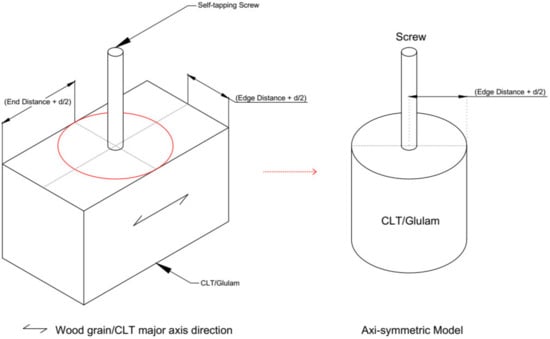
Figure 7.
Reduction of the wood-screw 3D system to an axisymmetric system.
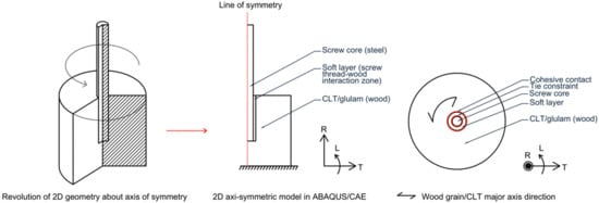
Figure 8.
Axisymmetric model in ABAQUS/CAE.
The thermal analysis module in ABAQUS/CAE is analogous to the moisture-swelling process in wood. Thus, thermal analysis using the ABAQUS standard solver was carried out to simulate the moisture-swelling process in CLT and glulam. In the thermal analysis, the temperature is analogous to the wood’s moisture content, and the coefficient of thermal expansion is analogous to the wood’s swelling coefficient. The uniform moisture content in the wood member was specified as a predefined constant-temperature field. For example, the whole wood member was assigned the 12% moisture content condition with a constant predefined temperature of 12 (unitless). The wood moisture swelling coefficient along the three orthotropic directions was defined as the orthotropic coefficient of thermal expansion values in ABAQUS/CAE.
For simulating the screw pull-out behavior under moisture content variation, an axial load was applied to the top surface of the screw core in the finite element model under (1) displacement control and (2) force control, with proper support and moisture content, that is, in terms of temperature and boundary conditions. The displacement-controlled axial load was applied by specifying a displacement boundary condition. The force-controlled axial load was applied by specifying a concentrated force acting on top of the screw core.
The screw core and the wood were modelled as linear elastic materials, and the soft layer was assigned the same material properties as the wood member [13]. The screw core was assigned isotropic material properties, whereas the wood was assigned orthotropic material properties. Local material orientation was assigned to the wood member, wherein the angular value was set per the average angle between the tangent to the annual rings and the horizontal direction of the CLT/glulam laminate’s end grain. The CAX4 elements of ABAQUS/CAE were used in the finite element model.
The screw core and the soft layer were rigidly connected with the “tie constraint” in ABAQUS/CAE, as the soft layer represents the integral threaded part of the screw embedded in the wood. A surface-based cohesive contact interaction was used to interconnect the external surface of the soft layer and the surrounding wood. In simpler terms, the soft layer was tied to the screw core on the inner side and cohesively bonded to the surrounding wood on the outer side, encapsulating the wood-screw thread interaction (Figure 8, right). The cohesive contact in ABAQUS/CAE utilizes the cohesive zone modelling (CZM) approach based on nonlinear fracture mechanics. The bottom end of the screw was modelled as a free edge, as it has a negligible effect on the stress distribution of the screw during axial loading [15]. The CZM approach is highly mesh-dependent, and a smaller element size is preferable. Mesh sizes of 0.5 mm for the 8 mm screw and 1 mm for the 13 mm screw were used for the screw core and the soft layer. For the CLT/glulam, a mesh size of 2 mm was used for all models. Both a free and structured mesh technique was used, and both techniques produced similar results. Enlarged pictures of the mesh of the models are shown in Figure 9.
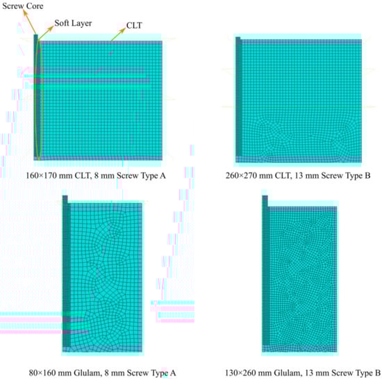
Figure 9.
Mesh for the different models.
The CZM approach can adequately describe the pull-out behavior of the screw during axial loading [13]. The cohesive contact interaction in ABAQUS/CAE requires three input parameters: an elastic behavior defined by the stiffness values, a damage initiation criterion, and a damage evolution model. The stiffness values along three directions were the normal direction (Knn), which is perpendicular to the screw longitudinal axis; and the two transverse (shear) directions (Kss and Ktt), wherein one was parallel to the screw longitudinal axis and one was parallel to the tangent to the cylindrical screw surface (Figure 10, right). The stiffness of the normal direction is less critical in this study as the axial loading is of primary interest here. The stiffness values along the two shear directions were assumed to be equal. The two shear directions correspond to the direction parallel to the screw axis and the direction tangent to the screw diameter. Since the 2D axisymmetric modelling technique is adopted here, the shear direction parallel to the screw axis affects the numerical solution. Assuming the same value of stiffness along the other shear direction tangent to the screw diameter has no effect on the numerical solution,, according to the traction separation law, the stiffness values relate the tractions (tn, ts, tt) in the three directions to the separation () in the respective directions (Figure 10, left).
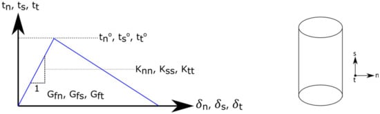
Figure 10.
Traction separation law and the directions in the cylindrical coordinate system.
The quadratic traction damage initiation criterion was used to determine the failure of the screw–wood interaction zone. The criterion is given by Equation (7):
Here, is the normal tension traction; and are the tractions in the two shear directions; and , and are the maximum tractions in the three directions when the separation is either purely normal to the screw interface or acts purely in the shear directions. The symbol ⟨ ⟩ signifies that a purely compressive displacement or a purely compressive stress state does not initiate damage [7].
Once the failure criterion is satisfied, the damage evolution model gives the stresses in the three directions. A linear energy-based softening model without considering mode-mixing was used as the damage evolution model. The total fracture energy per unit area (Gfn, Gfs, Gft) in each mode was equal, and only one value of the total fracture energy was defined. The fracture energy per unit area was calculated as:
The pressure–overclosure relationship type was set to “hard” contact, and the default constraint enforcement method was used to describe the normal behavior for the cohesive contact in ABAQUS/CAE. For the tangential behavior of cohesive contact, the “penalty friction” formulation with a friction coefficient of 0.2 was used [16]. Finally, the small sliding formulation was used in ABAQUS/CAE to define the cohesive contact interaction for better convergence.
3. Results and Discussion
3.1. Finite Element Input Material Properties from Tests
In the finite element model, the screw core was assigned isotropic elastic material properties. Young’s modulus for the screw core was determined from the self-tapping screw tensile tests, and Poisson’s ratio was taken as 0.3, as is usual for steel. Table 7 lists the mean values of Young’s modulus for each of the tested screw configurations. The plastic material properties were not used since the goal of the finite element model was to find the stress distribution of STS in the linear elastic range.
Table 7.
Self-tapping screw material properties (from Screw Tensile Tests).
CLT’s longitudinal and transverse layers were made of lumber of different grades and material properties. Also, the wood grain direction of CLT’s longitudinal and transverse layers are oriented in orthogonal directions. Thus, the wood member was partitioned into different layers to assign layer-specific material properties for CLT. The lumber used in all of the layers of glulam was of the same grade. The glulam was modelled as a single part without partitioning, and the same material properties were assigned to the whole glulam. The same material properties were used for the complete glulam specimen. Finally, the soft layer was assigned the same material properties as the wood member [13].
The wood member (CLT/glulam) was assigned orthotropic material properties. The input elastic material properties used to model the two types of CLT and glulam specimens were taken according to the stress grade of the laminates and research findings in the published literature [17]. As wood properties change significantly with the moisture content, the change in the elastic properties was considered by specifying temperature dependent moisture content. Temperature is analogous to the moisture content in ABAQUS/CAE thermal analysis formulation values of the elastic properties according to Gerhards [18]. These properties are mentioned in Table 8, Table 9, Table 10 and Table 11.
Table 8.
160 × 170 mm CLT material properties [18].
Table 9.
260 × 270 mm CLT material properties [18].
Table 10.
130 × 260 mm and 80 × 160 mm glulam material properties [18].
Table 11.
Swelling coefficient values for glulam and CLT (from Swelling Tests).
The swelling coefficients of the CLT and glulam along the three orthotropic directions were determined from the swelling tests previously described. For this purpose, the swelling strain versus moisture content plot was made for each group of samples along each of the wood’s orthotropic directions. The data points were fitted using a linear regression line. The slope of the regression line provided the value of the swelling coefficient (). The swelling strain versus moisture content plot and the fitted line for the glulam are shown in Figure 11. The L, R, and T subscripts in Table 11 refer to the primary orthotropic directions of wood, namely longitudinal, radial, and tangential directions, respectively.
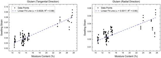
Figure 11.
Swelling strain versus moisture content plot for glulam (from Swelling Tests).
Specifying the proper local material orientation directions is essential to accurately model the withdrawal test specimens. The average angle between the tangent to the annual rings and the horizontal direction of the CLT/glulam laminate’s end grain was measured by hand. For each type of CLT and glulam product, a constant average value of the angle was used as the direction of the local material orientation for all the layers for modelling simplicity (Table 12).
Table 12.
Material orientation angle.
Withdrawal tests were conducted on the specimen configurations mentioned in Table 5. The specimens under conditioning settings numbers 1–3 in Table 5 were conditioned under constant EMC before and after the screw installation. The test results from these specimens were used as the input properties for the CZM contact interaction between the screw core and the wood member. The force–displacement curves of the withdrawal tests were used to determine the withdrawal strength, stiffness, and fracture energy per unit area.
The withdrawal strength of each screw was determined with Equation (3). The withdrawal stiffness was calculated according to Equation (6).
The failure mode of the specimen after the withdrawal tests is shown in Figure 12. The failure of the screws inside the samples were marked by pullout of the screws. The withdrawal failure is seen by the vertical pullout of the taped part of the screw, which was initially in contact with the top wood surface. None of the screws broke inside the wood after the tests.
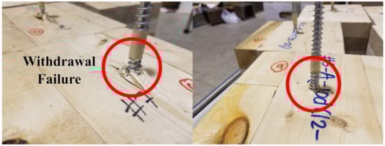
Figure 12.
Failure mode in a few specimens after the withdrawal tests.
As mentioned in the previous section, , and are the maximum tractions in the normal and the two shear directions, respectively. The maximum traction in the normal direction () is the least critical for the finite element model for axial loading condition and was set to an arbitrary value of 100 N/mm2. The maximum traction in the shear directions ( and ) was assigned the mean withdrawal strength value from the specimen’s withdrawal test results under conditioning settings numbers 1, 2, and 3, and for EMC 12%, 16%, and 21%, respectively. Similarly, the withdrawal test was also used to determine the fracture energy per unit area per Equation (8) for the linear energy-based softening model for the damage evolution. Mode mixing of the different fracture modes was not considered, and a constant fracture energy value (Gfn = Gfs = Gft = Gf) was specified to describe the damage evolution and ultimate failure in all three directions.
3.2. Finite Element Material Properties Calibration
The cohesive stiffness values, Knn, Kss, and Ktt affect the possibility of convergence and the ultimate load-carrying capacity of the screw during axial loading. For modelling the cohesive contact, these parameters have to be adjusted appropriately to make the finite element model representative of the actual behavior of screw–wood interaction. As the stiffness and traction of the normal direction are of the least importance in this study for axial loading conditions, the normal cohesive stiffness (Knn) value was set as an arbitrary constant value. The cohesive stiffness in the two shear directions was considered equal (Kss = Ktt). The value of the shear direction cohesive stiffness was changed until the ultimate load and the slope of the force-displacement curves from the FEA and the withdrawal tests were very close. The normal direction cohesive stiffness was assigned a significantly higher value than the cohesive stiffness values in the two shear directions. The normal direction cohesive stiffness values chosen for the different specimen configurations are given in Table 13.
Table 13.
Normal cohesive stiffness values.
The cohesive stiffness in the two shear directions was calibrated with the experimental withdrawal test results of the specimen under conditioning settings numbers 1, 2, and 3 for EMC 12%, 16%, and 21%, respectively. As a starting point, the input values for the cohesive stiffness were taken equal to the withdrawal stiffness from the withdrawal tests. The cohesive stiffness values were then scaled proportionately until a close match between the ultimate load and the slope of the initial linear portion of force-displacement curves from FEA and the withdrawal tests were achieved (Figure 13).
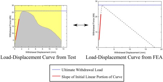
Figure 13.
Comparison of the load-displacement curve from finite element analysis (FEA) and withdrawal test.
Once the cohesive stiffness values at a constant EMC were calibrated, a moisture content-dependent cohesive interaction was defined to capture the effect of change of the cohesive parameters with moisture content. Then, the process of EMC change was incorporated, in terms of temperature field, in the finite element model along with the axial load. The load-displacement curve under varying EMC from the finite element model was verified with the load-displacement curve of specimen group 4 and group 5 in Table 5, which had different EMC in the two conditioning stages. The calibration and the verification process of the finite element model are illustrated in Figure 14.
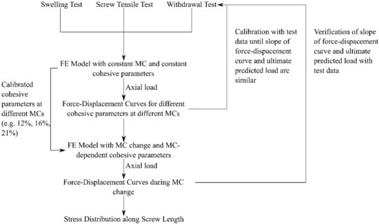
Figure 14.
Finite element model calibration and verification process.
The calibrated values of the cohesive stiffness are given in Table 14, Table 15, Table 16 and Table 17. The normal direction cohesive stiffness (Knn) was kept constant, and shear direction cohesive stiffness (Kss and Ktt) was varied proportionately with the withdrawal stiffness from the test. The slope of the initial linear portion of the force-displacement curve (Kser) and the maximum load capacity (Fmax) from the withdrawal test and FEA were compared. The scaled value of the withdrawal stiffness, which gave the lowest percentage difference of Kser and Fmax between the withdrawal test and finite element results, was chosen as the calibrated value of the cohesive stiffness.
Table 14.
130 × 260 mm Glulam calibrated values.
Table 15.
80 × 160 mm Glulam calibrated values.
Table 16.
260 × 270 mm CLT calibrated values.
Table 17.
160 × 170 mm CLT calibrated values.
The values of the other cohesive parameters (damage initiation criterion defined by the maximum traction and damage evolution model defined by the fracture energy per unit area) for the different specimen configurations are provided in Table 18, Table 19, Table 20 and Table 21.
Table 18.
130 × 260 mm Glulam damage initiation and evolution values.
Table 19.
80 × 160 mm Glulam damage initiation and evolution values.
Table 20.
260 × 270 mm CLT damage initiation and evolution values.
Table 21.
160 × 170 mm CLT damage initiation and evolution values.
3.3. Finite Element Analysis Steps, Loads, Boundary Conditions, and Predefined Fields
The standard solver in ABAQUS/CAE was used for all analyses. Only one analysis step was created for the finite element model for calibration after the initial step in ABAQUS/CAE. A displacement of 20 mm was applied to the top end of the screw in this step, and the top surface of the wood member was fixed (Figure 15) to create the pull–push loading condition, which is the boundary condition of the withdrawal test. For applying the displacement and ease of extracting the load-displacement curve, a reference point was defined on top of the screw (Figure 15). The reference point was tied with kinematic coupling to the top surface of the screw, and the displacement was applied to the reference point, yielding equal displacement at the top end of the screw and the reference point. The load-displacement curve of the top end of the screw was also extracted from this reference point.
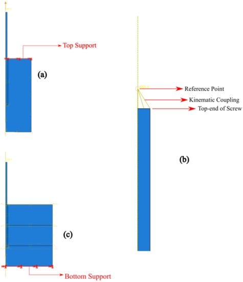
Figure 15.
(a) Top boundary condition, (b) reference point at the screw top, and (c) bottom boundary condition.
For verifying the finite element model, two analysis steps were created after the initial step. In the initial step, a constant predefined temperature (temperature is analogous to the EMC of wood) field was specified throughout the wood member and the soft layer geometry. The swelling/shrinkage of wood was simulated in the first step following the initial step by changing the value of the constant predefined temperature field specified in the initial step. Further, the bottom end of the wood member was kept fixed for stability and better convergence of the model, as shown in Figure 15 [14]. In the second step after the initial step, a pull-out displacement of 20 mm was applied on the top surface of the screw through the reference point, as done in the finite element model for calibration. Also, in this step, the bottom boundary condition was deactivated, whose primary purpose was to achieve convergence of the finite element model during the moisture swelling/shrinkage step. Instead, a fixed boundary condition was specified at the top surface of the wood member to simulate the pull–push loading condition. The predefined temperature field values used for simulating the moisture change of wood are shown in Table 22. Verification model number 1 was verified against the withdrawal test data of specimen conditioned under conditioning setting number 4 (12% → 21% EMC), and verification model number 2 was verified against specimen conditioned under conditioning setting number 5 (21% → 12% EMC) (Table 5). The two models aimed to investigate the case of wood wetting, an increase of EMC from 12% to 21%, and drying, a decrease of EMC from 21% to 12%, respectively. For verifying the finite element model, the same process as before was followed, that is, the slope of the initial linear portion of the force-displacement curve (Kser) and the maximum load capacity (Fmax) from the withdrawal test and FEA were compared.
Table 22.
Finite element verification models.
3.4. Finite Element Model Verification
The comparison between the load-displacement curve from the withdrawal test of specimen conditioned under conditioning setting numbers 4 and 5, and verification models 1 and 2, are illustrated in Table 23. It can be observed that the slope of the initial linear portion of the slope-displacement curve (Kser) for the drying cases (21% → 12% EMC change) from FEA is underpredicted compared to the test results. Reducing the wood moisture content by about 3% around fully threaded screws installed perpendicular to the wood’s grain direction can lead to critical tensile stresses in the wood member. The critical tensile stresses can lead to moisture-induced cracks and alter the composite action between the wood material and the thread of the screw [19]. This behavior was not accounted for in the finite element model, which might have led to the discrepancy. Furthermore, the finite element model did not consider stress relaxation due to mechano–sorptive effects [20]. These aspects are not investigated in this study and can be a topic for investigation in future research. The difference between the slopes from the test results and the FEA for the wetting cases (12% → 21% EMC change) was limited to about 20%. The ultimate load predicted from FEA and withdrawal tests deviated by a small amount, except for the wetting case of 80 × 160 mm glulam, with an 8 mm screw. However, since the domain of this study is within the linear elastic range, which is below ultimate load levels, the maximum load is less critical. Thus, from the difference in the force–displacement behaviour of the different specimen configurations, it can be concluded that the finite element model is more representative of the composite action between the wood material and the thread of the screw for the wetting cases than in the drying cases. Since the primary goal of this project is to investigate the stress distribution of the screw during wood-wetting (moisture swelling), the finite element model is adequate to that end.
Table 23.
Finite element model verification comparison.
3.5. Numerical Model Implementation
The combination of sufficiently high axial load value and moisture swelling of wood might cause the tensile failure of self-tapping screws. In two-member connections, like the one shown in Figure 16, the high axial load values might arise if the screw is installed very tightly, at a higher torque than required. The torque requirements for screw installation usually are provided by the screw manufacturers. In Figure 16, the side member is assumed to be sufficiently rigid to support the main member’s top surface. This condition then becomes similar to screw withdrawal under the pull–push loading condition. An over torque in the screw in this condition will induce an additional axial load in the screw. If one supposes that the main wood member undergoes moisture swelling in this over-torqued condition, then the numerical model described here can be used to predict the average axial stress distribution in the screw inside the main wood member due to the wood’s induced axial load and moisture swelling.
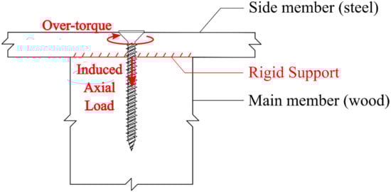
Figure 16.
Numerical model implementation in a two-member connection.
The induced axial load due to over-torquing of the screw can be estimated from the induced axial load and over-torque relationship, which can be investigated in future research. In this research, based on educated estimates of the maximum induced axial load from Matsubara et al. [21] and to achieve convergence of the finite element model, known load values were applied to the FE verification models 1 and 2. The load values, along with the moisture content change considered in the numerical model for the different specimen configurations, are provided in Table 24.
Table 24.
Axial load applied to the finite element model for analytical model verification.
Then, the average stress distribution of the screw along its length was determined from finite element verification models 1 and 2 (Table 22) at the different load values and moisture content changes listed in Table 24, which represented the case of axial loading of screw coupled with moisture content change of glulam/CLT. Paths were created in the screw core in the visualization module in ABAQUS/CAE to find the stress distribution. The starting point of the paths was at the entrant side of the screw, and the end point was at the bottom end of the screw (Figure 17). The stress distribution in the direction parallel to the screw (S22 in ABAQUS/CAE) was determined along these paths. They were averaged to get the average axial stress distribution in the screw.
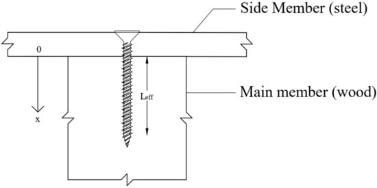
Figure 17.
Coordinate system for screw stress distribution.
Figure 17 illustrates the origin of the coordinate system for the screw stress distribution in a typical two-member connection with a self-tapping screw. As the pull–push loading condition is similar to the two-member connection where the side member is assumed to be sufficiently rigid to provide support to the top surface of the main wood member, the stress distribution given by the finite element model represents the average stress distribution of the screw in the x-direction with the starting point at the top surface of the main member and ending point at the effective penetration length (Leff). The stress distributions from FEA are illustrated in Figure 18 and Figure 19, respectively, for the cases of CLT and glulam wetting, an increase of moisture content from 12% to 21%, and drying, a decrease of moisture content from 21% to 12%, respectively.
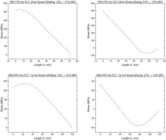
Figure 18.
Screw axial stress distribution in CLT.
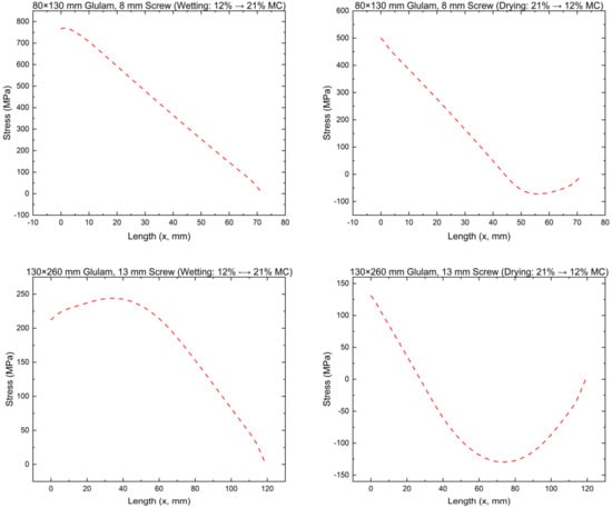
Figure 19.
Screw axial stress distribution in glulam.
From Figure 18 and Figure 19, the maximum stress in the 8 mm screw is about 800 MPa, and that in the 13 mm screw is about 250 MPa. The manufacturer-specified yield strength for the 8 mm screw was 1147 MPa and that of the 13 mm screw was 1000 MPa. Since the maximum stress was below the yield strength, the assumption of the screw being in the linear elastic regime during modelling is justified.
Stress in the screw for both CLT and glulam was non-zero at the screw entrant side, gradually decreasing to zero at the inner end of the screw. The maximum tensile stress was observed between the screw entrant side and the middle of the effective penetration length. The stress was gradually transferred from the screw to the surrounding wood with the increase in screw depth along the member. Thus, the maximum tensile stress in the screw was observed near the top. For the wood drying cases for CLT and glulam, it is seen that part of the stress in the screw that is in compression that is, negative stress. The compression region might be due to stress relaxation in the screw during wood drying. As already mentioned earlier, the modelling of wood drying cases might benefit from further research, which was outside the scope of this research.
4. Conclusions
This research aims to quantify the stress distribution in self-tapping screws in mass-timber products under moisture content change and axial load application. The numerical (finite element) modelling technique adopted here relies on input properties from screw tensile tests, CLT and glulam swelling tests, and withdrawal tests. The numerical model was calibrated and verified with experimental withdrawal test results. The numerical modelling technique described here only considers the linear elastic regime of the self-tapping screw’s stress–strain behaviour. In the future, the post-elastic regime of the behaviour self-tapping screw’s stress–strain behaviour can be included in the numerical modelling. The average axial stress distribution of the screw showed that the maximum stress was observed between the screw entrant side and the middle of the effective penetration length. At the induced loads from the over-torquing of the screws considered here, the maximum axial stress magnitude in the screw was lower than the tensile strength of the screw.
This research is the first attempt at investigating the axial stress arising in self-tapping screws under the simultaneous action of hygroscopic deformation of the wood and axial loading of self-tapping screws. The next step in this area of research is the development of an analytical model to predict the axial stress distribution in self-tapping screws in mass-timber products under moisture content change and axial load application.
Author Contributions
Conceptualization, C.N. and M.T.K.; methodology, M.T.K., C.N. and J.W.; software, M.T.K.; data curation, M.T.K.; formal analysis, M.T.K.; investigation, M.T.K.; visualization, M.T.K.; validation, M.T.K. and Y.H.C.; funding acquisition, Y.H.C. and C.N.; project administration, C.N. and Y.H.C.; resources, C.N., Y.H.C. and J.W.; supervision, C.N., Y.H.C. and J.W.; writing—original draft, M.T.K.; writing—review and editing, Y.H.C. and J.W. All authors have read and agreed to the published version of the manuscript.
Funding
This research was supported by a grant from the Natural Sciences and Engineering Research Council of Canada (NSERC) through the Industrial Research Chair (IRC) Program (Grant Number IRCPJ515081-16). In-kind support was also provided by FPInnovations in the form of staff time and use of their testing facility and Western Archrib in the form of test materials.
Data Availability Statement
The withdrawal test results of this study can be found here: https://doi.org/10.7939/r3-h8ad-eg08 (accessed on 10 November 2022). The rest of the data presented in this study are available on request from the corresponding author.
Acknowledgments
The authors gratefully acknowledge FPInnovations, MTC Solutions, Rothoblaas, Nordic Structures, Western Archrib, StructureCraft for their financial, technical support and valuable feedback.
Conflicts of Interest
The authors declare no conflict of interest.
References
- Dietsch, P.; Brandner, R. Self-tapping screws and threaded rods as reinforcement for structural timber elements—A state-of-the-art report. Constr. Build. Mater. 2015, 97, 78–89. [Google Scholar] [CrossRef]
- Jensen, J.L.; Koizumi, A.; Sasaki, T.; Tamura, Y.; Iijima, Y. Axially loaded glued-in hardwood dowels. Wood Sci. Technol. 2001, 35, 73–83. [Google Scholar] [CrossRef]
- Stamatopoulos, H.; Malo, K.A. Withdrawal capacity of threaded rods embedded in timber elements. Constr. Build. Mater. 2015, 94, 387–397. [Google Scholar] [CrossRef]
- Stamatopoulos, H.; Malo, K.A. Withdrawal stiffness of threaded rods embedded in timber elements. Constr. Build. Mater. 2016, 116, 263–272. [Google Scholar] [CrossRef]
- Gereke, T.; Niemz, P. Moisture-induced stresses in spruce cross-laminates. Eng. Struct. 2010, 32, 600–606. [Google Scholar] [CrossRef]
- Angst, V.; Malo, K.A. The effect of climate variations on glulam—An experimental study. Eur. J. Wood Wood Prod. 2012, 70, 603–613. [Google Scholar] [CrossRef]
- Simulia. ABAQUS Software; Dassault Systèmes: Aachen, Germany, 2020. [Google Scholar]
- CSA O86:19; Engineering Design in Wood. Canadian Standards Association: Toronto, ON, Canada, 2019.
- ASTM E8/E8M-22; Standard Test Methods for Tension Testing of Metallic Materials. ASTM International: West Conshohocken, PA, USA, 2022.
- ASTM E111-17; Standard Test Method for Young’s Modulus, Tangent Modulus, and Chord Modulus. ASTM International: West Conshohocken, PA, USA, 2017.
- EN 1382:2016; Timber Structures—Test Methods—Withdrawal Capacity of Timber Fasteners. European Committee for Standardization: Brussels, Belgium, 2016.
- Brandner, R.; Ringhofer, A.; Reichinger, T. Performance of axially-loaded self-tapping screws in hardwood: Properties and design. Eng. Struct. 2019, 188, 677–699. [Google Scholar] [CrossRef]
- Avez, C.; Descamps, T.; Serrano, E.; Léoskool, L. Finite element modelling of inclined screwed timber to timber connections with a large gap between the elements. Eur. J. Wood Wood Prod. 2016, 74, 467–471. [Google Scholar] [CrossRef]
- Bedon, C.; Sciomenta, M.; Fragiacomo, M. Mechanical Characterization of Timber-to-Timber Composite (TTC) Joints with Self-Tapping Screws in a Standard Push-Out Setup. Appl. Sci. 2020, 10, 6534. [Google Scholar] [CrossRef]
- Feldt, P.; Thelin, A. Glued-in Rods in Timber Structures: Finite Element Analyses of Adhesive Failure; Chalmers University of Technology: Gothenburg, Sweden, 2018. [Google Scholar]
- Murase, Y. Friction of Wood Sliding on Various Materials. J. Fac. Agric. Kyushu Univ. 1984, 28, 147–160. [Google Scholar] [CrossRef] [PubMed]
- Ross, R.J. Forest Products Laboratory USDA Forest Service. Wood Handbook: Wood as an Engineering Material; Forest Products Laboratory: Madison, WI, USA, 2010. [Google Scholar] [CrossRef]
- Gerhards, C.C. Effect of Moisture Content and Temperature on the Mechanical Properties of Wood: An Analysis of Immediate Effects. Wood Fiber Sci. 1982, 14, 4–36. [Google Scholar]
- Dietsch, P. Effect of reinforcement on shrinkage stresses in timber members. Constr. Build. Mater. 2017, 150, 903–915. [Google Scholar] [CrossRef]
- Toratti, T.; Svensson, S. Mechano-sorptive experiments perpendicular to grain under tensile and compressive loads. Wood Sci. Technol. 2000, 34, 317–326. [Google Scholar] [CrossRef]
- Matsubara, D.; Wakashima, Y.; Fujisawa, Y.; Shimizu, H.; Kitamori, A.; Ishikawa, K. Relationship between clamp force and pull-out strength in lag screw timber joints. J. Wood Sci. 2017, 63, 625–634. [Google Scholar] [CrossRef]


Disclaimer/Publisher’s Note: The statements, opinions and data contained in all publications are solely those of the individual author(s) and contributor(s) and not of MDPI and/or the editor(s). MDPI and/or the editor(s) disclaim responsibility for any injury to people or property resulting from any ideas, methods, instructions or products referred to in the content. |
© 2023 by the authors. Licensee MDPI, Basel, Switzerland. This article is an open access article distributed under the terms and conditions of the Creative Commons Attribution (CC BY) license (https://creativecommons.org/licenses/by/4.0/).