

Optimal Insulation Assessment, Emission Analysis, and Correlation Formulation for Indian Region

 , ,
, ,  ,
,  ,
,  , and
, and 
Abstract
1. Introduction
2. Materials and Methods
2.1. Building Wall Model
2.2. Building Wall Heating Load

| Fuel | Chemical Equation | Cf | η | Hu |
|---|---|---|---|---|
| Coal | C5.85H5.26O1.13S0.008N0.077 | 0.16610 $/kg | 0.65 | 21.113 × 10⁶ J/kg |
| Natural gas | C1.05H4O0.034N0.022 | 0.1305 $/m3 | 0.93 | 34.526 × 10⁶ J/m3 |
| Diesel | C7.3125 H10.407 O0.04 S0.026 N0.02 | 0.69981 $/kg | 0.80 | 42.911 × 10⁶ J/kg |
| Electricity | - | 0.08 $/kWh | 0.99 | 3.5990 × 10⁶ J/kWh |
2.3. Optimal Insulation Analysis
2.4. Environmental Analysis
3. Results and Discussion
3.1. Optimal Insulation Thickness
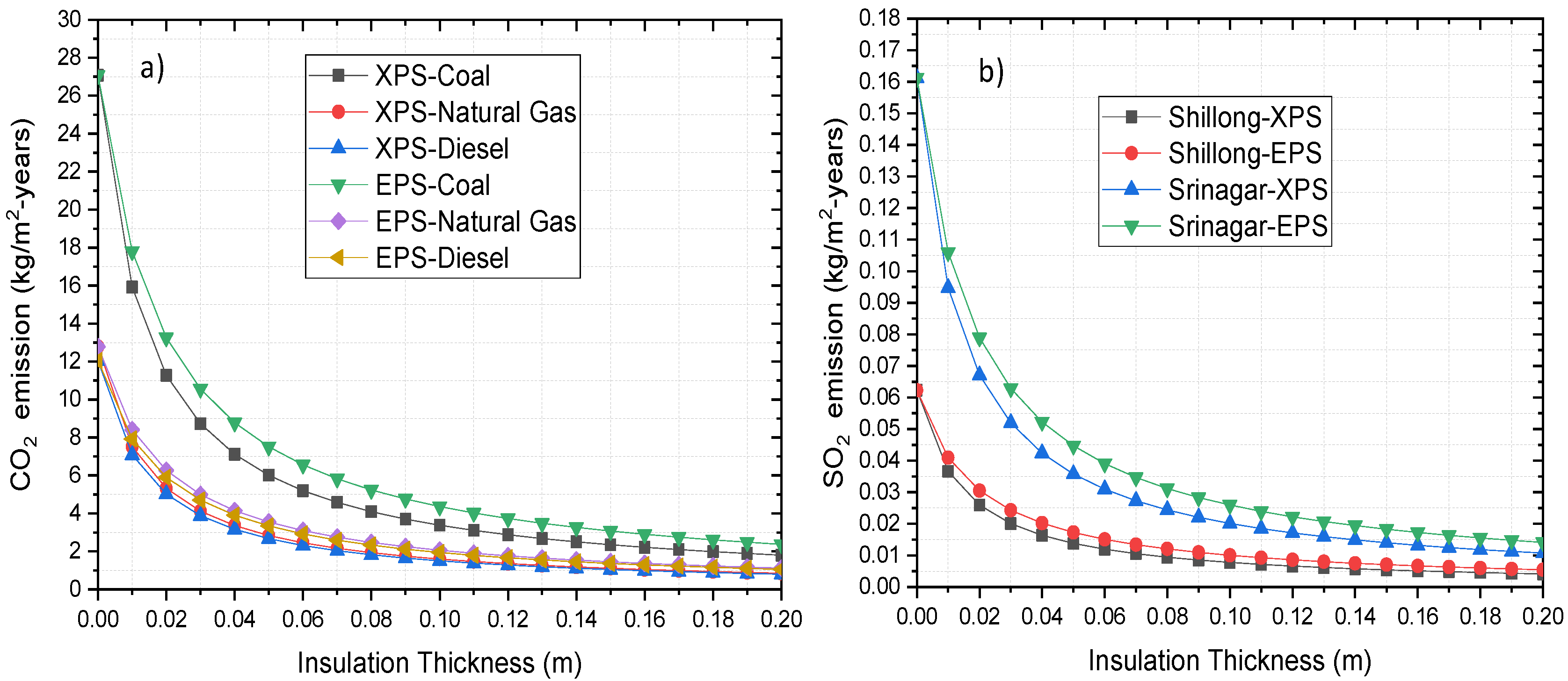
3.2. Environmental Analysis
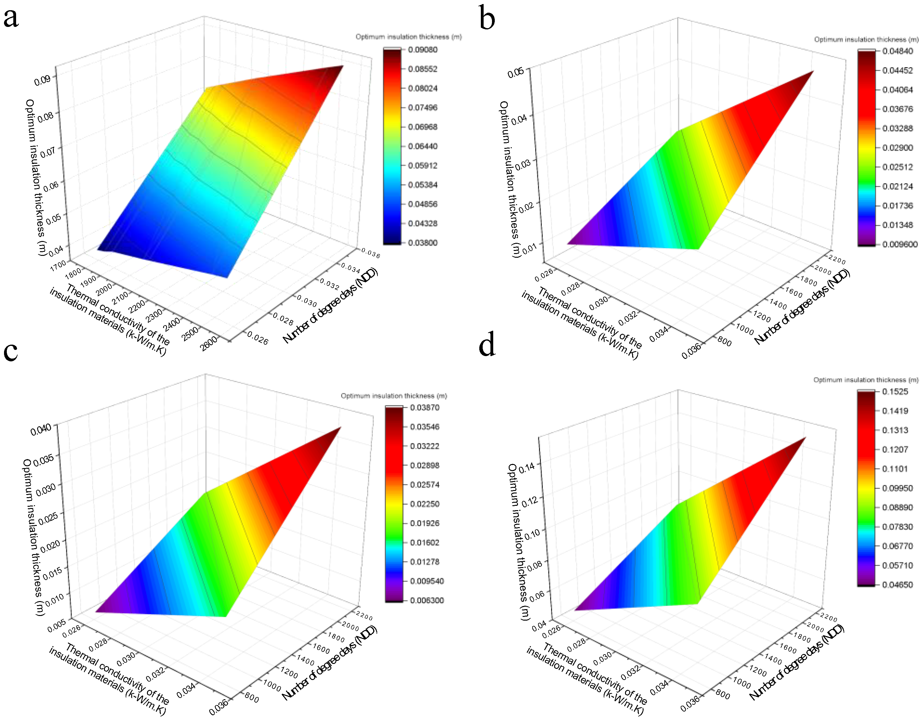
3.3. Degree Days and Correlations
4. Conclusions and Recommendations
- For sites situated in hot and dry, warm and humid, and composite climatic regions, the ranges of XPS insulation thickness, annual savings, and payback period for these regions were found as 0.0382–0.0484 m, 10.83–17.47 $/m2, and 1.93–2.36 years, respectively. Similarly, these ranges for EPS insulation thickness, annual savings, and payback period were 0.0728–0.0908 m, 12.79–19.9347 $/m2, and 1.49–1.79 years, respectively.
- For sites situated in cold climatic regions, the ranges of XPS insulation thickness, annual savings, and payback period were 0.0097–0.0834 m, 0.29–51.73 $/m2, and 1.24–6.52 years, respectively. The ranges for EPS insulation thickness, annual savings, and payback period were 0.0168–0.1522 m, 0.68–55.92 $/m2, and 0.95–4.85 years, respectively.
- The ranges of GHG emissions for XPS material with natural gas, coal, and diesel fuels were 9.67–11.28 kg/m2-year, 27.12–32.68 kg/m2-year, and 2.89–4.51 kg/m2-year, respectively. Similarly, the ranges of GHG emissions for EPS material with natural gas, coal, and diesel fuels were 5.39–9.17 kg/m2-year, 9.47–23.75 kg/m2-year, and 2.26–3.43 kg/m2-year, respectively.
- The optimal insulation thickness for XPS material was lower than that of EPS material, while the payback period and annual savings for XPS material were greater and lower, respectively, than those of EPS material in all the circumstances.
- XPS was proved to be more effective than EPS, and the correlations obtained could aid in the determination of optimal insulation thickness for a specific location based on the number of degree days.
Author Contributions
Funding
Institutional Review Board Statement
Informed Consent Statement
Data Availability Statement
Conflicts of Interest
Nomenclature
| Am | tropical monsoon climate | annual heat loss in unit area (J/m2-year) | |
| Aw | tropical savanna climate | actual interest rate | |
| Bsk | cold semi-arid (steppe) climate | inside air film thermal resistances (m2K/W) | |
| annual cooling energy cost ($/m2-year) | thermal resistance of insulation layer (m2K/W) | ||
| annual heating energy cost ($/m2-year) | outside air film thermal resistance (m2K/W) | ||
| cost of insulation in ($/m3) | sum of Ri.Rw.Ro (m2K/W) | ||
| cooling degree days (°C-days) | total thermal resistance of wall materials without insulation (m2K/W) | ||
| price of fuel ($/kg; $/m3) | annual savings ($/m2) | ||
| Csa | hot summer mediterranean climate | SO2 | sulfur dioxide |
| Csb | warm summer mediterranean climate | U | overall heat transfer coefficient (W/m2K) |
| total cost ($) | thickness of insulation material (m) | ||
| CO2 | carbon dioxide | optimum insulation thickness (m) | |
| Dbf | warm summer humid continental climate | XPS | extruded polystyrene |
| annual energy requirement (J/m2-year) | |||
| EPS | expanded polystyrene | Greek letters | |
| inflation rate | heating system efficiency | ||
| heating degree days (°C-days) | ΔT | temperature difference (°C) | |
| heating value of fuel (J/kg; J/m3; J/kwh) | |||
| interest rate | Subscripts | ||
| thermal conductivity of insulation material (W/m K) | A | annual | |
| LCA | lifecycle cost analysis | C | cooling |
| M | molar weight of fuel | H | heating |
| amount of fuel consumed per year (kg/m2-year) | i | inside | |
| N | lifetime (years) | izo | insulation |
| number of (degree days (°C-days) | o | outside | |
| payback period (years) | opt | optimum | |
| PWF | present worth factor | t | total |
| heat loss (MJ m2 year−1) | w | wall |
References
- Kallioğlu, M.A.; Ercan, U.; Avcı, A.S.; Fidan, C.; Karakaya, H. Empirical Modeling between Degree Days and Optimum Insulation Thickness for External Wall. Energy Sources Part A Recovery Util. Environ. Eff. 2020, 42, 1314–1334. [Google Scholar] [CrossRef]
- Altun, A.F. Determination of Optimum Building Envelope Parameters of a Room Concerning Window-to-Wall Ratio, Orientation, Insulation Thickness and Window Type. Buildings 2022, 12, 383. [Google Scholar] [CrossRef]
- Wang, H.; Huang, Y.; Yang, L. Integrated Economic and Environmental Assessment-Based Optimization Design Method of Building Roof Thermal Insulation. Buildings 2022, 12, 916. [Google Scholar] [CrossRef]
- Shaik, S.; Gorantla, K.; Ghosh, A.; Arumugam, C.; Maduru, V.R. Energy Savings and Carbon Emission Mitigation Prospective of Building’s Glazing Variety, Window-to-Wall Ratio and Wall Thickness. Energies 2021, 14, 8020. [Google Scholar] [CrossRef]
- Skaar, C.; Gaarder, J.-E.; Bunkholt, N.S.; Sletnes, M. Energy Upgrading of Basement Exterior Walls: The Good, the Bad and the Ugly. Buildings 2023, 13, 133. [Google Scholar] [CrossRef]
- Kallioğlu, M.A.; Sharma, A.; Chinnasamy, V.; Chauhan, R.; Singh, T. Optimum Insulation Thickness Assessment of Different Insulation Materials for Mid-Latitude Steppe and Desert Climate (BSH) Region of India. Mater. Today Proc. 2020, 44, 4421–4424. [Google Scholar] [CrossRef]
- Xu, H.; Ding, J.; Li, T.; Mu, C.; Gu, X.; Wang, R. A Study on Optimum Insulation Thickness in Walls of Chinese Solar Greenhouse for Energy Saving. Agronomy 2022, 12, 1104. [Google Scholar]
- Nyers, J.; Kajtar, L.; Tomić, S.; Nyers, A. Investment-Savings Method for Energy-Economic Optimization of External Wall Thermal Insulation Thickness. Energy Build. 2015, 86, 268–274. [Google Scholar] [CrossRef]
- Liu, X.; Chen, Y.; Ge, H.; Fazio, P.; Chen, G. Determination of Optimum Insulation Thickness of Exterior Wall with Moisture Transfer in Hot Summer and Cold Winter Zone of China. Procedia Eng. 2015, 121, 1008–1015. [Google Scholar] [CrossRef]
- Yuan, J.; Farnham, C.; Emura, K.; Alam, M.A. Proposal for Optimum Combination of Reflectivity and Insulation Thickness of Building Exterior Walls for Annual Thermal Load in Japan. Build. Environ. 2016, 103, 228–237. [Google Scholar] [CrossRef]
- Dombaycı, Ö.A. The Environmental Impact of Optimum Insulation Thickness for External Walls of Buildings. Build. Environ. 2007, 42, 3855–3859. [Google Scholar] [CrossRef]
- Kaynakli, O.; Bademlioglu, A.H.; Ufat, H.T. Determination of Optimum Insulation Thickness for Different Insulation Applications Considering Condensation. Teh. Vjesn. 2018, 25, 32–42. [Google Scholar]
- Bolattürk, A. Determination of Optimum Insulation Thickness for Building Walls with Respect to Various Fuels and Climate Zones in Turkey. Appl. Therm. Eng. 2006, 26, 1301–1309. [Google Scholar] [CrossRef]
- Mahlia, T.M.I.; Taufiq, B.N.; Masjuki, H.H. Correlation between Thermal Conductivity and the Thickness of Selected Insulation Materials for Building Wall. Energy Build. 2007, 39, 182–187. [Google Scholar] [CrossRef]
- Sisman, N.; Kahya, E.; Aras, N.; Aras, H. Determination of Optimum Insulation Thicknesses of the External Walls and Roof (Ceiling) for Turkey’s Different Degree-Day Regions. Energy Policy 2007, 35, 5151–5155. [Google Scholar] [CrossRef]
- Shanmuga Sundaram, A.; Bhaskaran, A. Optimum Insulation Thickness of Walls for Energy-Saving in Hot Regions of India. Int. J. Sustain. Energy 2014, 33, 213–226. [Google Scholar] [CrossRef]
- Mishra, S.; Usmani, J.A.; Varshney, S. Energy Saving Analysis in Building Walls through Thermal Insulation System. Int. J. Eng. Res. Appl. 2012, 2, 128–135. [Google Scholar]
- Raza, A.; Aggarwal, V. Evaluation of Optimum Insulation Thickness for Cost Saving of Wall Design in India. Available online: https://www.researchsquare.com/article/rs-1565499/v1.pdf (accessed on 13 October 2022).
- Singh, H.K.; Prakash, R.; Shukla, K.K. Economic Insulation Thickness of External Walls in Hot and Composite Regions of India. In Proceedings of the Global Conference on Renewable Energy GCRE2016, Patna, India, 4–6 March 2016; p. 6. [Google Scholar]
- Clark, H.; Wu, H. The Sustainable Development Goals: 17 Goals to Transform Our World. In Furthering Work United Nations; UN: New York, NY, USA, 2016; pp. 36–54. [Google Scholar]
- Kottek, M.; Grieser, J.; Beck, C.; Rudolf, B.; Rubel, F. World Map of the Köppen-Geiger Climate Classification Updated. Meteorol. Z. 2006, 15, 259–263. [Google Scholar] [CrossRef]
- Rubel, F.; Brugger, K.; Haslinger, K.; Auer, I. The climate of the European Alps: Shift of very high resolution Köppen-Geiger climate zones 1800–2100. Meteorol. Z. 2017, 26, 115–125. [Google Scholar] [CrossRef]
- JRC Photovoltaic Geographical Information System (PVGIS)—European Commission. Available online: https://re.jrc.ec.europa.eu/pvg_tools/en/#MR (accessed on 15 February 2022).
- Szokolay, S. Introduction to Architectural Science; Routledge: London, UK, 2012. [Google Scholar]
- Shehadi, M. Energy Consumption Optimization Measures for Buildings in the Midwest Regions of USA. Buildings 2018, 8, 170. [Google Scholar] [CrossRef]
- Kon, O.; Caner, İ. The Effect of External Wall Insulation on Mold and Moisture on the Buildings. Buildings 2022, 12, 521. [Google Scholar] [CrossRef]
- Aditya, L.; Mahlia, T.M.I.; Rismanchi, B.; Ng, H.M.; Hasan, M.H.; Metselaar, H.S.C.; Muraza, O.; Aditiya, H.B. A Review on Insulation Materials for Energy Conservation in Buildings. Renew. Sustain. Energy Rev. 2017, 73, 1352–1365. [Google Scholar] [CrossRef]
- Standard, T. 825 (TS 825). In Thermal Insulation in Buildings; Official Gazette (23725): Ankara, Turkey, 1999; Volume 14. [Google Scholar]
- Nellis, G.; Klein, S. Heat Transfer; Cambridge University Press: Cambridge, UK, 2008; ISBN 1-139-47661-0. [Google Scholar]
- Qian, X.; Lee, S.W.; Yang, Y. Heat Transfer Coefficient Estimation and Performance Evaluation of Shell and Tube Heat Exchanger Using Flue Gas. Processes 2021, 9, 939. [Google Scholar] [CrossRef]
- Statistics, E.; Central Statistics Office, Ministry of Statistics and Programme Implementation. Govt. India New Delhi (22nd Issue) 2015. Available online: www.mospi.gov (accessed on 8 February 2022).
- Cengel, Y. Heat and Mass Transfer: Fundamentals and Applications; McGraw-Hill Higher Education: Columbus, OH, USA, 2014. [Google Scholar]
- Kurekci, N.A. Determination of Optimum Insulation Thickness for Building Walls by Using Heating and Cooling Degree-Day Values of All Turkey’s Provincial Centers. Energy Build. 2016, 118, 197–213. [Google Scholar] [CrossRef]
- Llantoy, N.; Chàfer, M.; Cabeza, L.F. A Comparative Life Cycle Assessment (LCA) of Different Insulation Materials for Buildings in the Continental Mediterranean Climate. Energy Build. 2020, 225, 110323. [Google Scholar] [CrossRef]
- Hasan, A. Optimizing Insulation Thickness for Buildings Using Life Cycle Cost. Appl. Energy 1999, 63, 115–124. [Google Scholar] [CrossRef]
- Inflation Rate in India 1984–2024. Available online: https://www.statista.com/statistics/271322/inflation-rate-in-india/ (accessed on 16 August 2020).
- SBI—Loans, Accounts, Cards, Investment, Deposits, Net Banking—Personal Banking. Available online: https://sbi.co.in/ (accessed on 23 February 2021).
- Yildiz, A.; Gurlek, G.; Erkek, M.; Ozbalta, N. Economical and Environmental Analyses of Thermal Insulation Thickness in Buildings. J. Therm. Sci. Technol. 2008, 28, 25–34. [Google Scholar]
- Ozel, M. Cost Analysis for Optimum Thicknesses and Environmental Impacts of Different Insulation Materials. Energy Build. 2012, 49, 552–559. [Google Scholar] [CrossRef]
- Asadi, S.; Amiri, S.S.; Mottahedi, M. On the Development of Multi-Linear Regression Analysis to Assess Energy Consumption in the Early Stages of Building Design. Energy Build. 2014, 85, 246–255. [Google Scholar] [CrossRef]
- Chapra, S.C.; Canale, R.P. Numerical Methods for Engineers; McGraw-Hill Higher Education: Boston, MA, USA, 2010. [Google Scholar]
- Qian, X.; Lee, S.; Soto, A.; Chen, G. Regression Model to Predict the Higher Heating Value of Poultry Waste from Proximate Analysis. Resources 2018, 7, 39. [Google Scholar] [CrossRef]
- Alghoul, S.K.; Gwesha, A.O.; Naas, A.M. The Effect of Electricity Price on Saving Energy Transmitted from External Building Walls. Energy Res. J. 2016, 7, 1–9. [Google Scholar] [CrossRef]
- Alsayed, M.F.; Tayeh, R.A. Life Cycle Cost Analysis for Determining Optimal Insulation Thickness in Palestinian Buildings. J. Build. Eng. 2019, 22, 101–112. [Google Scholar] [CrossRef]
- Ucar, A.; Balo, F. Effect of Fuel Type on the Optimum Thickness of Selected Insulation Materials for the Four Different Climatic Regions of Turkey. Appl. Energy 2009, 86, 730–736. [Google Scholar] [CrossRef]


| No. | City | Latitude (Degree) | Altitude (m) | HDD (°C/Year) | CDD (°C/Year) | Average Temp. (°C/Year) | Process | Climate |
|---|---|---|---|---|---|---|---|---|
| 1 | Jaisalmer | 29.90 N | 225 | 43 | 2565 | 27.38 | Cooling | Hot dry |
| 2 | Kota | 25.20 N | 271 | 87 | 2123 | 26 | Cooling | Hot dry |
| 3 | Mumbai | 19.07 N | 14 | 0 | 2092 | 26.82 | Cooling | Warm humid |
| 4 | Chennai | 13.08 N | 6.7 | 0 | 2485 | 27.82 | Cooling | Warm humid |
| 5 | Bhubaneswar | 20.29 N | 58 | 1 | 1895 | 26.24 | Cooling | Warm humid |
| 6 | New Delhi | 28.61 N | 216 | 267 | 1791 | 24.34 | Cooling | Composite |
| 7 | Lucknow | 26.85 N | 123 | 144 | 1842 | 24.89 | Cooling | Composite |
| 8 | Patna | 25.59 N | 53 | 75 | 1791 | 25.02 | Cooling | Composite |
| 9 | Srinagar | 34.08 N | 1585 | 2109 | 26 | 13.14 | Heating | Cold |
| 10 | Shillong | 25.57 N | 1525 | 815 | 0 | 16.04 | Heating | Cold |
| Wall Type | Density (kg·m−3) | Thickness (m) | Thermal Conductivity (W/m·K) | Thermal Resistance (m2K/W) | Thermal Resistance RTW (Total Wall) (m2K/W) |
|---|---|---|---|---|---|
| Inner plaster | 1200 | 0.02 | 0.85 | 0.0230 | 0.548 |
| Hollow brick | 750 | 0.13 | 0.45 | 0.2880 | |
| Outer plaster | 1100 | 0.02 | 0.85 | 0.0230 | |
| R inside | - | - | - | 0.1670 | |
| R outside | - | - | - | 0.0450 |
| Materials | Xopt (m) | Annual Savings ($/m2) | Payback Period (Years) | Annual Savings Rate (%) |
|---|---|---|---|---|
| Jaisalmer | ||||
| XPS | 0.0484 | 17.47 | 1.96 | 40.28 |
| EPS | 0.0908 | 19.94 | 1.49 | 31.83 |
| Kota | ||||
| XPS | 0.0428 | 13.63 | 2.16 | 43.71 |
| EPS | 0.0809 | 15.82 | 1.64 | 34.66 |
| Mumbai | ||||
| XPS | 0.0424 | 13.36 | 2.18 | 43.99 |
| EPS | 0.0802 | 15.54 | 1.65 | 34.89 |
| Chennai | ||||
| XPS | 0.0475 | 16.77 | 1.99 | 40.84 |
| EPS | 0.0891 | 19.19 | 1.51 | 32.29 |
| Bhubaneswar | ||||
| XPS | 0.0401 | 11.70 | 2.29 | 45.88 |
| EPS | 0.0754 | 13.73 | 1.74 | 36.46 |
| New Delhi | ||||
| XPS | 0.0382 | 10.83 | 2.36 | 46.99 |
| EPS | 0.0728 | 12.79 | 1.79 | 37.38 |
| Lucknow | ||||
| XPS | 0.0389 | 11.25 | 2.33 | 46.44 |
| EPS | 0.0741 | 13.25 | 1.77 | 36.92 |
| Patna | ||||
| XPS | 0.0382 | 10.83 | 2.36 | 46.99 |
| EPS | 0.0728 | 12.79 | 1.79 | 37.38 |
| Fuel | Materials | Xopt (m) | Annual Savings ($/m2) | Payback Period (Years) | Annual Savings Rate (%) |
|---|---|---|---|---|---|
| Srinagar | |||||
| Natural gas | XPS | 0.0242 | 4.36 | 3.27 | 60.39 |
| EPS | 0.0483 | 5.63 | 2.47 | 48.80 | |
| Coal | XPS | 0.0188 | 2.62 | 3.86 | 67.70 |
| EPS | 0.0387 | 3.62 | 2.91 | 55.29 | |
| Diesel | XPS | 0.0834 | 51.73 | 1.24 | 27.06 |
| EPS | 0.1522 | 55.92 | 0.95 | 21.15 | |
| Shillong | |||||
| Natural gas | XPS | 0.0097 | 0.69 | 5.49 | 83.69 |
| EPS | 0.0227 | 1.25 | 4.11 | 70.57 | |
| Coal | XPS | 0.0063 | 0.29 | 6.52 | 90.66 |
| EPS | 0.0168 | 0.68 | 4.85 | 78.19 | |
| Diesel | XPS | 0.0465 | 16.05 | 2.03 | 41.44 |
| EPS | 0.0873 | 18.42 | 1.54 | 32.79 | |
| Fuel | Model | a | b | c | R2 | SSE | RMSE |
|---|---|---|---|---|---|---|---|
| Electricity | 26 | −0.1039 | 4.161 | 1.823 × 10⁻⁵ | 0.9943 | 3.443 × 10⁻⁵ | 0.0016 |
| Natural gas | 27 | −0.05929 | 2.061 | 1.549 × 10⁻⁵ | 0.9604 | 3.08 × 10⁻⁵ | 0.0055 |
| Coal | 28 | −0.05079 | 1.689 | 1.329 × 10⁻⁵ | 0.9598 | 2.209 × 10⁻⁵ | 0.0047 |
| Diesel | 29 | −0.1509 | 6.089 | 3.934 × 10⁻⁵ | 0.9661 | 1.96 × 10⁻⁴ | 0.0140 |
| Low | Mid | High | |||||||||||
|---|---|---|---|---|---|---|---|---|---|---|---|---|---|
| Case | Location | Reference | Ref. Value | Relative Error (Er) % | |||||||||
| Developed Model | Previous Models | ||||||||||||
| Country | City | Reference | Climate | NDD | Process | Fuel | Material | k (W/m·K) | xopt (m) | Developed Eq. for Corresponding Fuel | Mahlia et al. [14] | Sisman et al. [15] | |
| 1 | India | Jaisalmer | Present Study | Bwh | 2565 | Cooling | Electricity | XPS | 0.0260 | 0.0484 | 0.0536 | 0.0047 | 6.6422 |
| 2 | India | Jaisalmer | Present Study | Bwh | 2565 | Cooling | Electricity | EPS | 0.035 | 0.0908 | 0.0261 | 0.3736 | 3.0736 |
| 3 | India | Kota | Present Study | Bsh | 2123 | Cooling | Electricity | XPS | 0.026 | 0.0428 | 0.0033 | 0.1255 | 6.4946 |
| 4 | India | Kota | Present Study | Bsh | 2123 | Cooling | Electricity | EPS | 0.035 | 0.0809 | 0.0064 | 0.2969 | 2.965 |
| 5 | India | Mumbai | Present Study | Aw | 2092 | Cooling | Electricity | XPS | 0.026 | 0.0424 | 0.0006 | 0.1361 | 6.4819 |
| 6 | India | Mumbai | Present Study | Aw | 2092 | Cooling | Electricity | EPS | 0.035 | 0.0802 | 0.0048 | 0.2908 | 2.9555 |
| 7 | India | Chennai | Present Study | Aw | 2485 | Cooling | Electricity | XPS | 0.026 | 0.0475 | 0.0429 | 0.0141 | 6.6034 |
| 8 | India | Chennai | Present Study | Aw | 2485 | Cooling | Electricity | EPS | 0.035 | 0.0891 | 0.0238 | 0.3616 | 3.0534 |
| 9 | India | Bhubaneswar | Present Study | Aw | 1895 | Cooling | Electricity | XPS | 0.026 | 0.0401 | 0.0327 | 0.2013 | 6.3431 |
| 10 | India | Bhubaneswar | Present Study | Aw | 1895 | Cooling | Electricity | EPS | 0.035 | 0.0754 | 0.011 | 0.2456 | 2.9053 |
| 11 | India | New Delhi | Present Study | Aw | 1791 | Cooling | Electricity | XPS | 0.026 | 0.0382 | 0.0342 | 0.261 | 6.3874 |
| 12 | India | New Delhi | Present Study | Aw | 1791 | Cooling | Electricity | EPS | 0.035 | 0.0728 | 0.021 | 0.2187 | 2.8764 |
| 13 | India | Lucknow | Present Study | Cwa | 1842 | Cooling | Electricity | XPS | 0.026 | 0.0389 | 0.0277 | 0.2383 | 6.4096 |
| 14 | India | Lucknow | Present Study | Cwa | 1842 | Cooling | Electricity | EPS | 0.035 | 0.0741 | 0.0157 | 0.2324 | 2.8898 |
| 15 | India | Patna | Present Study | Cwa | 1791 | Cooling | Electricity | XPS | 0.026 | 0.0382 | 0.0342 | 0.261 | 6.3874 |
| 16 | India | Patna | Present Study | Cwa | 1791 | Cooling | Electricity | EPS | 0.035 | 0.0728 | 0.021 | 0.2187 | 2.8764 |
| 17 | India | Srinagar | Present Study | Bwk | 2109 | Heating | Natural gas | XPS | 0.026 | 0.0242 | 0.1142 | 0.9906 | 12.189 |
| 18 | India | Srinagar | Present Study | Bwk | 2109 | Heating | Natural gas | EPS | 0.035 | 0.0483 | 0.0577 | 0.1776 | 5.6081 |
| 19 | India | Srinagar | Present Study | Bwk | 2109 | Heating | Coal | XPS | 0.026 | 0.0188 | 0.1251 | 1.5623 | 15.9773 |
| 20 | India | Srinagar | Present Study | Bwk | 2109 | Heating | Coal | EPS | 0.035 | 0.0387 | 0.0606 | 0.4698 | 7.2474 |
| 21 | India | Srinagar | Present Study | Bwk | 2109 | Heating | Diesel | XPS | 0.026 | 0.0834 | 0.0837 | 0.4224 | 2.827 |
| 22 | India | Srinagar | Present Study | Bwk | 2109 | Heating | Diesel | EPS | 0.035 | 0.1522 | 0.0461 | 0.6263 | 1.0971 |
| 23 | India | Shillong | Present Study | Am | 815 | Heating | Natural gas | XPS | 0.026 | 0.0097 | 0.2866 | 3.9661 | 15.0769 |
| 24 | India | Shillong | Present Study | Am | 815 | Heating | Natural gas | EPS | 0.035 | 0.0227 | 0.122 | 1.5057 | 5.8699 |
| 25 | India | Shillong | Present Study | Am | 815 | Heating | Coal | XPS | 0.026 | 0.0063 | 0.3722 | 6.6463 | 23.7534 |
| 26 | India | Shillong | Present Study | Am | 815 | Heating | Coal | EPS | 0.035 | 0.0168 | 0.1403 | 2.3857 | 8.2825 |
| 27 | India | Shillong | Present Study | Am | 815 | Heating | Diesel | XPS | 0.026 | 0.0465 | 0.1511 | 0.0359 | 2.3537 |
| 28 | India | Shillong | Present Study | Am | 815 | Heating | Diesel | EPS | 0.035 | 0.0873 | 0.0799 | 0.3485 | 0.7863 |
| 29 | Libya | Tripoli | [43] | Csa | 492 | Cooling | Electricity | EPS | 0.037 | 0.069 | 0.1452 | 0.127 | 0.5453 |
| 30 | Turkey | Adana | [33] | Csa | 874 | Heating | Natural gas | XPS | 0.024 | 0.069 | 0.9462 | 0.3093 | 1.3823 |
| 31 | Turkey | Adana | [33] | Csa | 874 | Heating | Natural gas | EPS | 0.035 | 0.069 | 0.6176 | 0.1757 | 1.3823 |
| 32 | Turkey | Adana | [33] | Csa | 874 | Heating | Natural gas | Glass wool | 0.05 | 0.024 | 1.3874 | 2.9438 | 5.849 |
| 33 | Turkey | Adana | [33] | Csa | 874 | Heating | Natural gas | Rock wool | 0.048 | 0.035 | 0.5193 | 1.5124 | 3.6965 |
| 34 | Turkey | Adana | [33] | Csa | 874 | Heating | Natural gas | Polyurethane | 0.017 | 0.05 | 1.2143 | 0.0014 | 2.2875 |
| 35 | Turkey | Adana | [33] | Csa | 874 | Heating | Coal | XPS | 0.031 | 0.048 | 0.7253 | 0.0774 | 2.4245 |
| 36 | Turkey | Adana | [33] | Csa | 874 | Heating | Coal | EPS | 0.044 | 0.017 | 1.0671 | 3.4737 | 8.6692 |
| 37 | Turkey | Adana | [33] | Csa | 874 | Heating | Coal | Glass wool | 0.061 | 0.031 | 1.0598 | 3.5427 | 4.3025 |
| 38 | Turkey | Adana | [33] | Csa | 874 | Heating | Coal | Rock wool | 0.059 | 0.044 | 0.3745 | 1.9833 | 2.7358 |
| 39 | Turkey | Adana | [33] | Csa | 874 | Heating | Coal | Polyurethane | 0.022 | 0.061 | 1.0331 | 0.2187 | 1.6947 |
| 40 | Palestine | Jericho | [44] | Csa | 1989 | Cooling | Electricity | Polystyrene | 0.038 | 0.059 | 0.5325 | 0.0527 | 4.1762 |
| 41 | Palestine | Hebron | [44] | Dfb | 456 | Cooling | Electricity | Polystyrene | 0.038 | 0.022 | 1.8404 | 1.8231 | 3.5769 |
| 42 | Palestine | Jerusalem | [44] | Csa | 768 | Cooling | Electricity | Polystyrene | 0.038 | 0.049 | 0.3913 | 0.2675 | 2.0433 |
| 43 | Palestine | Tulkarem | [44] | Csa | 1066 | Cooling | Electricity | Polystyrene | 0.038 | 0.057 | 0.2913 | 0.0896 | 2.3492 |
| 44 | Palestine | Gaza | [44] | Bsh | 1097 | Cooling | Electricity | Polystyrene | 0.038 | 0.062 | 0.1962 | 0.0017 | 2.1463 |
| 45 | Palestine | Bethelem | [44] | Csa | 971 | Cooling | Electricity | Polystyrene | 0.038 | 0.053 | 0.3561 | 0.1719 | 2.3573 |
| 46 | Palestine | Jenin | [44] | Csa | 1399 | Cooling | Electricity | Polystyrene | 0.038 | 0.068 | 0.1716 | 0.0866 | 2.4454 |
| 47 | Palestine | Nablus | [44] | Csa | 854 | Cooling | Electricity | Polystyrene | 0.038 | 0.052 | 0.3412 | 0.1944 | 2.1064 |
| 48 | Turkey | Ağrı | [45] | Dsb | 4423 | Heating | Coal | XPS | 0.031 | 0.0261 | 1.3123 | 0.9815 | 20.3638 |
| 49 | Turkey | Ağrı | [45] | Dsb | 4423 | Heating | Natural gas | XPS | 0.031 | 0.0314 | 1.3284 | 0.6471 | 16.7578 |
| 50 | Turkey | Aydın | [45] | Csa | 1213 | Heating | Coal | XPS | 0.031 | 0.0022 | 7.0408 | 22.508 | 94.6422 |
| 51 | Turkey | Aydın | [45] | Csa | 1213 | Heating | Natural gas | XPS | 0.031 | 0.005 | 3.6781 | 9.3435 | 41.0826 |
| 52 | Turkey | Elazığ | [45] | Dsa | 2653 | Heating | Coal | XPS | 0.031 | 0.019 | 0.9383 | 1.722 | 18.9686 |
| 53 | Turkey | Elazığ | [45] | Dsa | 2653 | Heating | Natural gas | XPS | 0.031 | 0.0182 | 1.5108 | 1.8416 | 19.8463 |
| 54 | Turkey | Kocaeli | [45] | Cfa | 1786 | Heating | Coal | XPS | 0.031 | 0.0113 | 1.2394 | 3.5768 | 23.9209 |
| 55 | Turkey | Kocaeli | [45] | Cfa | 1786 | Heating | Natural gas | XPS | 0.031 | 0.0106 | 2.044 | 3.879 | 25.5666 |
| 56 | India | - | [19] | Hot and humid | 1288 | Cooling | Electricity | XPS | 0.036 | 0.028 | 1.476 | 1.0891 | 6.8622 |
| 57 | India | - | [19] | Hot and dry | 1111 | Cooling | Electricity | XPS | 0.036 | 0.031 | 1.1323 | 0.8869 | 5.3529 |
| 58 | India | - | [19] | Composite | 1121 | Cooling | Electricity | XPS | 0.036 | 0.031 | 1.1382 | 0.8869 | 5.396 |
| 59 | India | Dehradun | [17] | Cfa | 3587 | Heating | Natural gas | XPS | 0.033 | 0.057 | 0.1278 | 0.0519 | 7.3542 |
| 60 | India | Dehradun | [17] | Cfa | 3587 | Heating | Natural gas | EPS | 0.031 | 0.073 | 0.1758 | 0.2915 | 5.5231 |
Disclaimer/Publisher’s Note: The statements, opinions and data contained in all publications are solely those of the individual author(s) and contributor(s) and not of MDPI and/or the editor(s). MDPI and/or the editor(s) disclaim responsibility for any injury to people or property resulting from any ideas, methods, instructions or products referred to in the content. |
© 2023 by the authors. Licensee MDPI, Basel, Switzerland. This article is an open access article distributed under the terms and conditions of the Creative Commons Attribution (CC BY) license (https://creativecommons.org/licenses/by/4.0/).
Share and Cite
Kallioğlu, M.A.; Yılmaz, A.; Sharma, A.; Mohamed, A.; Dobrotă, D.; Alam, T.; Khargotra, R.; Singh, T. Optimal Insulation Assessment, Emission Analysis, and Correlation Formulation for Indian Region. Buildings 2023, 13, 569. https://doi.org/10.3390/buildings13020569
Kallioğlu MA, Yılmaz A, Sharma A, Mohamed A, Dobrotă D, Alam T, Khargotra R, Singh T. Optimal Insulation Assessment, Emission Analysis, and Correlation Formulation for Indian Region. Buildings. 2023; 13(2):569. https://doi.org/10.3390/buildings13020569
Chicago/Turabian StyleKallioğlu, Mehmet Ali, Ahmet Yılmaz, Ashutosh Sharma, Ahmed Mohamed, Dan Dobrotă, Tabish Alam, Rohit Khargotra, and Tej Singh. 2023. "Optimal Insulation Assessment, Emission Analysis, and Correlation Formulation for Indian Region" Buildings 13, no. 2: 569. https://doi.org/10.3390/buildings13020569
APA StyleKallioğlu, M. A., Yılmaz, A., Sharma, A., Mohamed, A., Dobrotă, D., Alam, T., Khargotra, R., & Singh, T. (2023). Optimal Insulation Assessment, Emission Analysis, and Correlation Formulation for Indian Region. Buildings, 13(2), 569. https://doi.org/10.3390/buildings13020569