Structural Identification from Operational Modal Analysis: The Case of Steel Structures

Abstract

In the case of old existing structures where the cultural value is very high, structural health analyses and investigations would be better performed without damages or service interruptions. Thus, modal analysis aimed at identifying eigenfrequencies and eigenmodes represents a very effective strategy to identify structural characteristics. In this paper, an innovative strategy to identify structural parameters exploiting the modal information obtained from operational modal analysis is proposed. The importance of the structural modeling in the problem formulation is highlighted. In the case of a simply supported beam, it was possible to assess the beam steel elastic modulus, while in the case of a cantilever beam, some constraint characteristics have been evaluated as well. In the steel frame case, the focus was on the constraint conditions of the structure determining the flexural stiffness of the springs representing the column base constraints. The method performances are promising for applications in larger structures such as bridges and buildings.

1. Introduction

A large part of European building constructions have exceeded their service life or require careful structural health analyses. This is particularly important in Italy where historical monuments are spread around the whole country and the main infrastructures were built in the 1950s and 1960s [1,2]. In this specific case and in case of monumental buildings where the cultural value is very high [3], structural health analyses and investigations should be performed while preserving the existing structures.

Thus, modal analysis aimed at identifying eigenfrequencies and eigenmodes represents a very effective strategy to identify structural characteristics. In particular, operational modal analysis (OMA) is a modal parameters identification technique based on vibration data collected when the structure is in service conditions [4]. Practically, OMA considers random environmental vibrations and cyclic loads on the structure as unknown sources of excitation. The easiest OMA technique is the peak picking (PP) method [5,6]. It is a frequency domain technique in which the natural frequencies are pointed as peaks in the power spectrum. Basic assumptions are that damping is low and the modes are well-separated. More complex methods such as frequency domain decomposition (FDD) [7], time domain decomposition (TDD) [8], and stochastic subspace identification (SSI) [9] are out of the scopes of this paper.

An emerging strategy to measure the modal properties without adding accelerometers to the system is 3D laser vibrometry, see [10,11,12], which has the main advantage in taking the measures from a distance. This can be useful in case of large structures that are not easily reachable.

The developments of computational mechanics allow to accurately model the structural behavior considering many parameters that often are not easily known. Indeed, a direct measure of these parameters would require high costs and would not always be compatible with the preservation of historical and monumental buildings.

For this reason, it is often more effective to formulate an inverse problem in which the eigenfrequencies measured through OMA represent a benchmark and the model parameters can be tuned in order to obtain numerical eigenfrequencies similar to the benchmark ones. Actually, this approach requires a good optimization strategy and presents quite a high computational cost. Usually, this optimization problem is represented by target functions that are neither continuous nor monotonic; consequently, the use of a heuristic algorithm such as simulated annealing [13,14,15], genetic algorithms [16,17], differential evolution [18], ant colony [19], and particle swarm [20] becomes mandatory.

Recently, [21] reported on an inverse problem for the structural identification of floor diaphragms using a perturbation approach. The study [22] presented an identification problem for a reinforced concrete, tall building based on model updating and experimental modal analysis. In [23], the authors showed the dynamic identification of the Baptistery of San Giovanni in Firenze (Italy) based on OMA and frequency domain decomposition.

With specific attention to steel structures, an interesting structural identification was performed for a steel footbridge in [24], while [25] presented an experimental modal analysis for a steel arch bridge. More recently, [26] presented an image-based operational modal analysis aimed at damage detection in a steel frame, and [27] reported on truss steel bridge damage identification through experimental modal analysis.

This paper presents a strategy to identify structural parameters exploiting the modal information obtained from OMA and developing an inverse problem in which the outcomes of experimental modal analyses are considered a known input while the structural parameters of a mathematical model representing the real structure are unknown. The use of the simulated annealing algorithm to minimize the difference between experimental eigenfrequencies and those obtained by the model represents a novelty in the literature. The importance of the structural modeling in the problem formulation is highlighted. This methodology has been applied to three different steel structures characterized by increasing complexity.

After this brief introduction, the paper is organized as follows: Section 2 presents a general description of the simulated annealing algorithm necessary for the proposed methodology, while the methodologies for structural identification are shown in Section 3. Finally, some conclusive remarks are drawn in Section 4.

2. Simulated Annealing

Initially introduced as a generic heuristic technique for discrete optimization, simulated annealing (SA) has become a widely used tool to tackle optimization problems in a wide range of application areas such as business, medicine, and engineering [13,14,15].

Also known as a local search algorithm, the SA does not find the optimal solution but provides an approximate solution very close to the optimal one. This is performed through a stochastic and iterative procedure in which the local search starts from an initial current configuration and the choice of the next configuration is randomly generated (randomized exploration).

The methodological process is inspired by the behavior of fluids when subjected to processing involving controlled cooling, as in the production of large crystals. Indeed, if cooling occurs rapidly, the crystal lattice may be affected by defects such as cracking or fracture. The annealing process, on the other hand, involves gradual cooling, bringing the structure of the crystal to an optimal and stable configuration according to the principle of minimum potential energy.

For each temperature value T belonging to a defined range, the solid can reach thermal equilibrium in which the probability of being in a state with energy $E$ is defined by the Boltzmann distribution [28]:

$$Pr\left\{\mathbf{E}=E\right\}=\frac{1}{Z\left(T\right)}{e}^{-E/k_B T}$$

(1)

where $Z\left(T\right)$ is a normalization factor (also called partition function), which depends on the temperature $T$; $k_B$ is the Boltzmann constant; and $e^{-E/k_{B}T}$ is the Boltzmann factor.

The stochastic component of the method lies in the application of the Monte Carlo method to generate successive configurations through small random perturbations starting from a current configuration with energy $E_i$.

According to the Metropolis Criterion [29], the energy difference:

$$\Delta E=E_j-E_i$$

(2)

between the perturbed j-th configuration $E_j$and the current i-th configuration $E_i$ can be:

$\Delta E\le 0$, then the j-th configuration replaces the previous one as it has a lower potential energy:

$\Delta E>0$, then the j-th configuration is accepted with probability $e^{-\Delta E/k_{B}T}$.

The algorithm, therefore, does not exclude a priori the analysis of worst-case solutions but admits them with a decreasing probability as the temperature decreases. Indeed, the exponential function is governed by the relationship between the change in energy of two configurations and the temperature. The probability that the j-th worst solution will be confirmed decreases as $\Delta E$ increases. In addition, the temperature, T, is high in the early stages of the algorithm and low in the final stages.

Therefore, since as temperature decreases, the Boltzmann distribution concentrates on the lower energy states, at the end of the cooling process only the lower energy states are likely to occur.

One of the most important features of the SA is the robustness of the algorithm, due to the possibility of easily dealing with nonlinear problems with many variables, despite the presence of strongly discontinuous functions. However, it has some disadvantages:

-

it is not possible to know whether the solution found, which is a local minimum, coincides with the global minimum or how different the two values are;

-

the quality of the local minimum obtained depends on the initial configuration chosen, but no criterion establishes a way of selecting a starting point that allows good solutions to be obtained;

-

it may require very long computational times that cannot be predicted a priori.

Switching from the physical problems to combinatorial optimization problems [30], the energy becomes the cost function $C$, the temperature is a control parameter $c$, the particle configurations become the values of the problem variables and the search for the lowest energy state becomes the search for the solution that minimizes the cost function.

In order to ensure that the algorithm performs the calculation cycles, it is necessary to define the initial value of the control parameter $c_0$, the final value of the control parameter $c_f$ that stops the algorithm, and the decrement law of the control parameter. The choice of $c_0$ must be made in such a way that, in the initial phase of the algorithm, all configurations must be approved, while on reaching $c_f$, any deterioration of the solution must not be accepted. Furthermore, the law of variation of the control parameter must be chosen considering that a higher cooling rate corresponds to a higher number of iterations to reach a new equilibrium state: this naturally influences the computational effort. If the control parameter is initially set equal to $c_0=0$, the SA operates similarly to a local minimum search algorithm.

A Matlab^TM 2013 version of SA is available in the literature [31], which initially requires parameters to be defined.

Table 1. Parameters used in the optimization process.

Parameter	Entity
$c_0$	1
$c_f$	${10}^{-8}$
$k_B$	1
N	150
Variation law of $c$	$c_{k+1}={\left(c_f/c_0\right)}^{1/N} · c_k$

shows the input value adopted in this work.

3. Structural Identification

3.1. Proposed Method

The structural identification strategy proposed in this work is based on the following steps:

-

Execution of operational modal analysis (OMA) focused on the extraction of modal eigenfrequencies from output only experimental data.

-

Development of theoretical (analytical and numerical) structural models for dentification purpose.

-

Identification of unknown structural parameters (x₁, x₂,… x_j) that minimize the following error function.

$$e=\sqrt{{{\displaystyle \sum }}_i^n{\left(\frac{f_{is}-f_{in}\left(x_1,x_2,\dots x_j\right)}{f_{is}}\right)}^2}$$

(3)

where f_is is the i-th experimental eigenfrequency and f_in is the corresponding theoretical one obtained from a model depending on the set of chosen unknown parameters (x₁, x₂,… x_j). The latter represent properly chosen unknown characteristics of the structure such as structural stiffness, material mechanical property, boundary stiffness, etc. The optimization of Equation (3) can be performed using the SA algorithm. In this way, it is possible to identify the unknown parameters that are the target of the structural identification problem. In this procedure, the experimental eigenfrequencies represent the benchmark necessary for the structural identification strategy.

3.2. Experimental Apparatus

The proposed methodology will be tested using the experimental modal data obtained from steel beams and a steel frame built in the Materials Strength Laboratory of the University of Cagliari.

The experimental apparatus was composed of:

-

Accelerometer sensor PCB 393C characterized by a sensitivity of 101.9 mV/(m/s²) and a frequency range (±5%): 0.025 to 800 Hz, see Figure 1.

-

Data acquisition hardware: Dymas 24. It is composed of a central unit with a CPU that has the task of managing the acquisition process, synchronization of the sensors, and data storage. The system is characterized by 30 channels managed by 5 acquisition cards. Each card has an internal memory of 1 GB and is equipped with a DSP (on-board) processor that autonomously manages the functions of digitization and amplification of the inputs and filters the signals. Each card is connected to the CPU by USB connections, see Figure 1.

-

Dedicated software: DymaSoft^TM 3.6.3 for the connection and configuration of the system and VibroSoft^TM 3.2.19 aimed at displaying and processing the recorded data.

Given the beam characteristics, in order to have a harmonic force with variable frequencies, we built a home-made vibrodyne, see Figure 2 and

Table 2. Vibrodyne dimensions.

h	120 mm	mm
dV	110 mm	mm
da	3 mm	mm
Mr	50 gr	gr
e	20 mm	mm

. It was made from a tin container in which a steel rotation axis with an eccentric mass was inserted. A potentiometer was adopted to control the rotation speed. The dynamic forces applied by this system can be expressed as:

$$\overrightarrow{F}\left(t\right)=M_r·{\omega }_r^2\mathit{sin}\left({\omega }_r^2 t\right)$$

(4)

where $M_r$ represents the rotating mass and ${\omega }_r^2$ is its rotation frequency. The experimental modal analysis tests were developed using the hypothesis of white noise in the loading vibration. For this reason, the vibrodyne was used at different rotation speeds that were randomly varied by the users. This was conducted in order to perform a pure OMA without knowing the dynamic loading characteristics.

The experimental tests were developed considering first a steel beam characterized by different boundary conditions and then a more complex steel frame.

3.3. Steel Beams

The experimental modal analysis was developed while considering two beams with different boundary conditions. In the first case, the beam was simply supported, see Section 3.3.1, and in the second, it was clamped on one side and free on the other to analyze a cantilever beam, see Section 3.3.2.

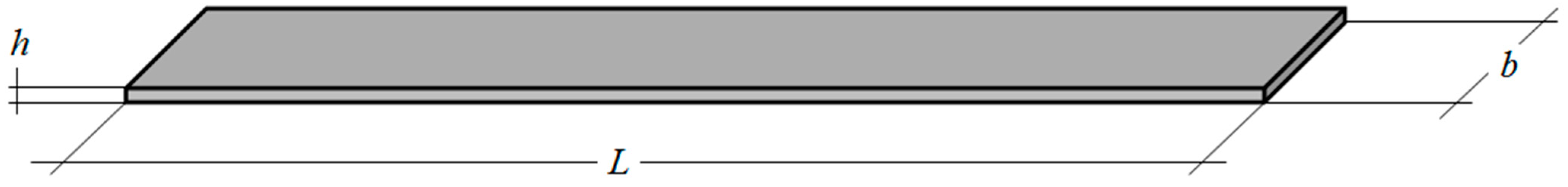
3.3.1. Simply Supported Beam

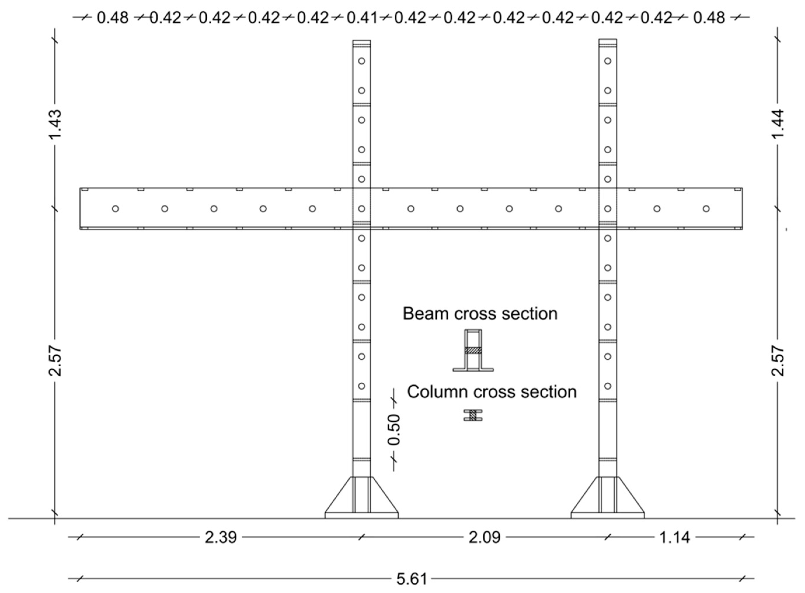
The simply supported beam’s geometrical characteristics are reported in Figure 3. Its density is 7746.90 kg/m³, the steel longitudinal elastic modulus E_s-real is 203 GPa, while dimensions are L = 1499.00 mm, b = 118.82 mm, and h = 6.39 mm.

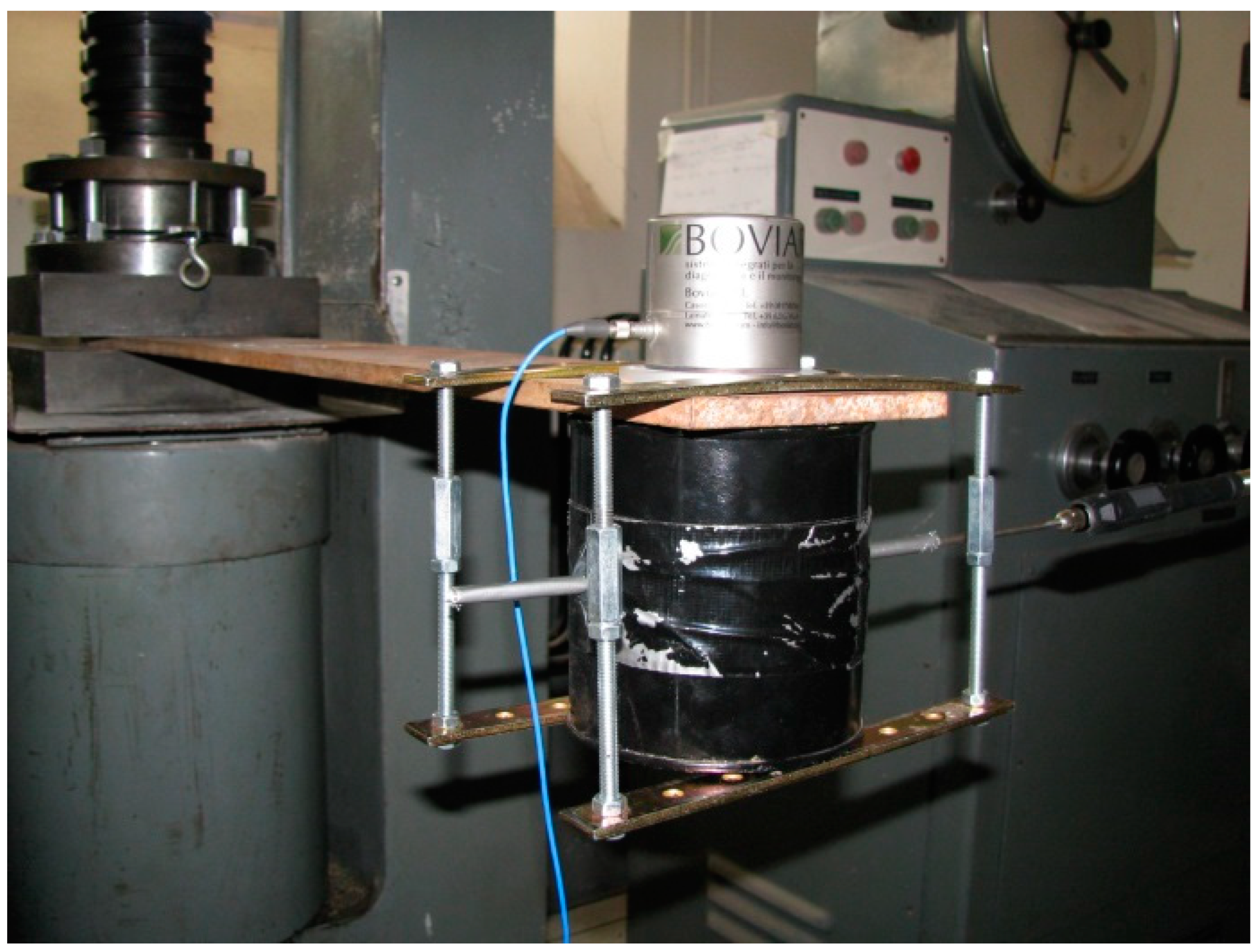
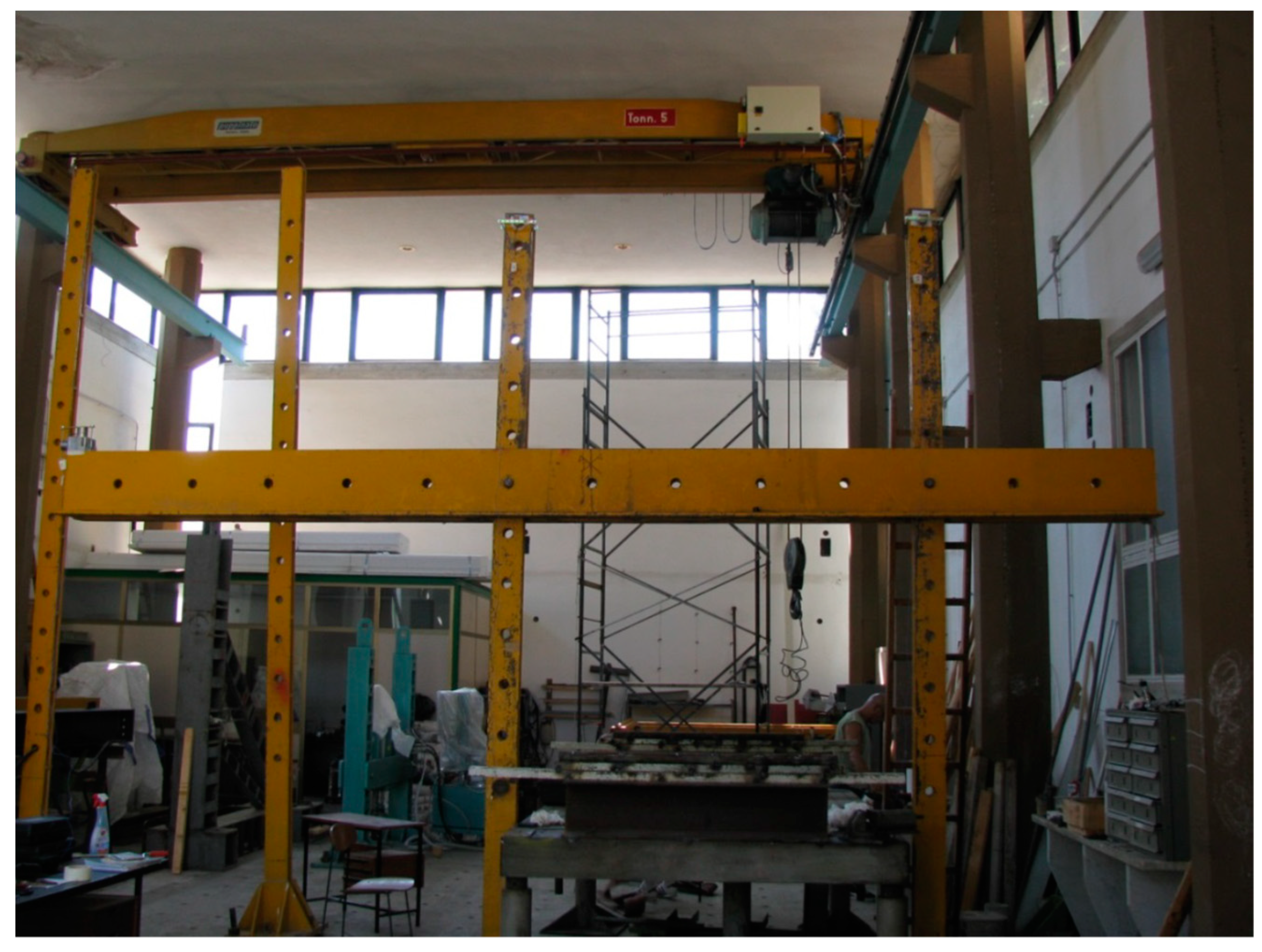
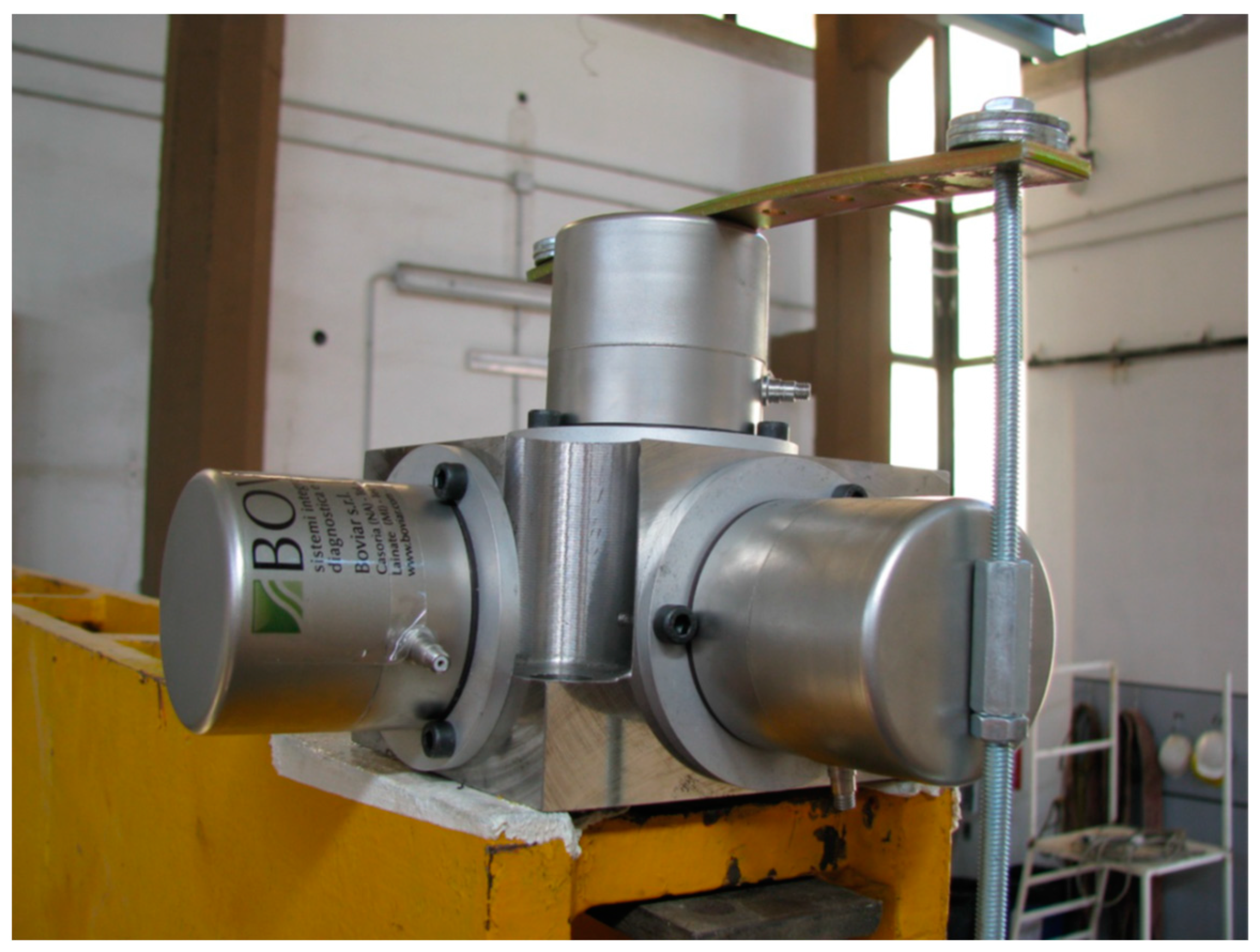
Figure 3 presents the experimental set up. The positions of the vibrodyne and accelerometer were chosen in order to avoid the nodes of the beam eigenmodes, i.e., the sections that do not undergo any displacement during the vibrations in natural modes. The accelerometer is located 435 mm from the right side and symmetrically to the vibrodyne which was placed 435 mm from the left side, see Figure 4.

The vibrodyne was used by varying randomly the rotation speed. In this way, it was possible to record several samples with different harmonic force. In order to have a statistical consistency, the test was repeated 6 times with a sampling frequency equal to 500 Hz.

Actually, since an OMA approach was adopted, the random rotation speed of the vibrodyne was approximated as a white noise.

The acceleration response time histories were obtained for each case and the first 5 flexural modal frequencies were identified (see

Table 3. Experimental eigenfrequencies of the simply supported beam and the corresponding standard deviation (SD).

Mode	fi,s [Hz]	SD [Hz]
1	6.00	0.03
2	23.23	0.16
3	57.52	0.38
4	100.12	0.18
5	142.93	0.12

and Figure 5) using the fast Fourier transform [32] and the peak picking method [5]. As is well-known, see [33], this technique is based on the low damping and well-separated modes hypotheses that can be assumed for this case.

The matrix of the cross-spectral density (spectral matrix) presents on its diagonal terms the real valued autospectral densities and it is defined as:

$$\mathit{G}\left(f\right)=E_{xp}\left[\mathit{A}\left(f\right){\mathit{A}}^H\left(f\right)\right]$$

(5)

where $\mathit{A}\left(f\right)$ is a vector containing the acceleration responses in the frequency domain and ${\mathit{A}}^H\left(f\right)$ is the complex conjugate transpose matrix, while $E_{xp}$ represents the expected value. In the Peak Picking approach, in the neighbourhood of an eigenfrequency $f_r$ the spectral matrix is approximated by:

$$\mathit{G}\left(f_r\right)\approx {\alpha }_r{\Phi }_r{\Phi }_r^{\mathrm{H}}$$

(6)

where ${\alpha }_r$ is a parameter depending on the damping ratio, considering eigenfrequency, excitation spectra, and modal participation factor, see [33,34]. ${\Phi }_r$ is the mode shape vector corresponding to frequency $f_r$. In this paper, the beam eigenfrequencies were identified from the resonant peak in the autospectral density using the PP approach. The method was quite efficient since the considered eigenmodes were well-detached, as is typical for simple structures such as beams. In case of eigenmodes close to each other, it is possible to filter the accelerometric data in order to improve the accuracy or to use different approaches such as FDD [7], TDD [8], or SSI [9].

In order to perform the structural identification, we developed an analytical beam model based on the Euler–Bernoulli theory with the aim of identifying the longitudinal elastic modulus. It was previously measured with a quasi-static test, so its benchmark value is known.

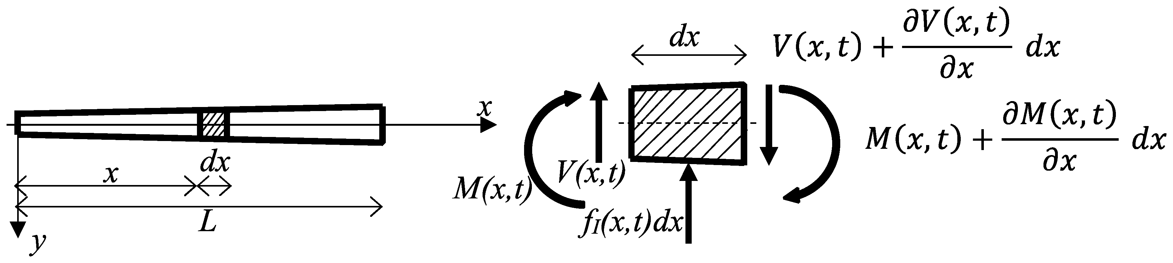
The Euler–Bernoulli beam theory takes into account bending stiffness and transversal inertia and assumes that plane sections remain plane and perpendicular to the beam axis after deformation, see Figure 6. In case of free vibration, the equation of motion is:

$$\frac{{\partial }^{2}M}{\partial x^2}-\mu \frac{{\partial }^{2}v}{\partial t^2}=0$$

(7)

where $\mu$ represents the mass per unit lenght of the beam, M is the bending moment, v is the deflection, and t is the time.

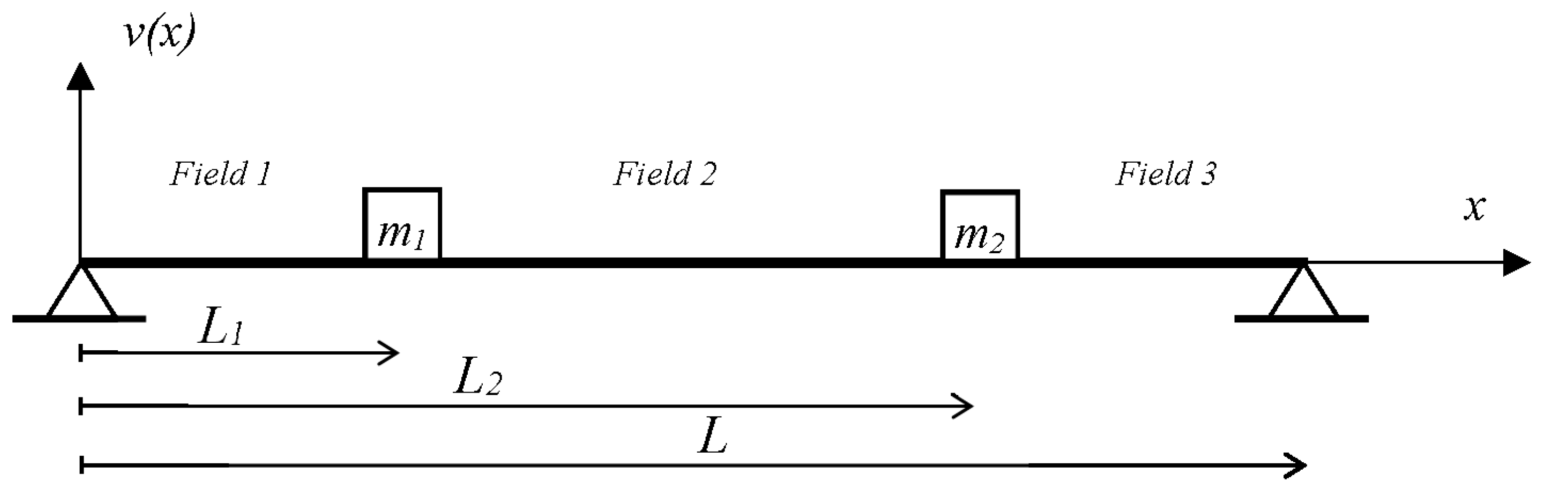
Given the mass of the accelerometer (0.89 kg), of the vibrodyne (0.93 kg), and of the beam (8.82 kg), it is necessary to take into account the exact position of these masses also in the analytical model. For this reason, the Euler–Bernoulli beam Equation (7) has been integrated considering the three different fields separated by the two lumped masses of the vibrodyne and of the accelerometer, see Figure 7.

In each field, by means of the separation of variables technique, it is possible to distinguish between the time harmonic solution and the space variation of the solution:

$$v \left(x,t\right)={{\displaystyle \sum }}_j^{\infty }{v}_j\left(x\right) \mathit{sin}\left({\omega }_{j}t\right)$$

(8)

where $t$ is the time, $x$ represents the position along the beam, $v_j$ is the j-th eigenmode, and ${\omega }_j$ is the i-th natural circular frequency of the beam. The relationship between frequencies and circular frequencies is: $\frac{{\omega }_j}{2\pi }=f_{i}n$. Given ${\lambda }_j=L^4\frac{\mu {\omega }_j^2}{EJ}$ and considering the three fields of integration, it is possible to prove (see [35]) that:

$$v_{1j}\left(x\right)=A_{1j}\mathit{cos}\left(\frac{{\lambda }_{j}x}{L}\right)+A_{2j}\mathit{sin}\left(\frac{{\lambda }_{j}x}{L}\right)+A_{3j}\mathit{cos}\mathit{h}\left(\frac{{\lambda }_{j}x}{L}\right)+A_{4j}\mathit{sin}\mathit{h}\left(\frac{{\lambda }_{j}x}{L}\right)$$

$$v_{2j}\left(x\right)=A_{5j}\mathit{cos}\left(\frac{{\lambda }_{j}x}{L}\right)+A_{6j}\mathit{sin}\left(\frac{{\lambda }_{j}x}{L}\right)+A_{7j}\mathit{cos}\mathit{h}\left(\frac{{\lambda }_{j}x}{L}\right)+A_{8j}\mathit{sin}\mathit{h}\left(\frac{{\lambda }_{j}x}{L}\right)$$

(9)

$$v_{3j}\left(x\right)=A_{9j}\mathit{cos}\left(\frac{{\lambda }_{j}x}{L}\right)+A_{10j}\mathit{sin}\left(\frac{{\lambda }_{j}x}{L}\right)+A_{11j}\mathit{cos}\mathit{h}\left(\frac{{\lambda }_{j}x}{L}\right)+A_{12j}\mathit{sin}\mathit{h}\left(\frac{{\lambda }_{j}x}{L}\right)$$

where v_ij denotes the spatial solution of the i-th field related to the j-th eigenmodes, and A_ij represents the generic integration constant that can be determined using the boundary conditions. The 12 boundary conditions expressing static and cinematic compatibility are presented in the following system of equations expressed in matrix notation:

$$D ·A=0$$

(10)

where D is the matrix of the system, and A is the vector containing the unknown integration constant.

In order to avoid the uniqueness of null solution, it is necessary that:

$$\det D=0$$

(11)

Equation (11) represents the frequency equation whose roots are the circular eigenfrequencies of the beam. Unfortunately, this equation can be solved only with a numerical approach; consequently, it is not possible to find a close form solution. For this reason, an iterative semianalytical algorithm was developed in Matlab^TM 2013 [36] that finds the eigenfrequency of the beam using Equation (11).

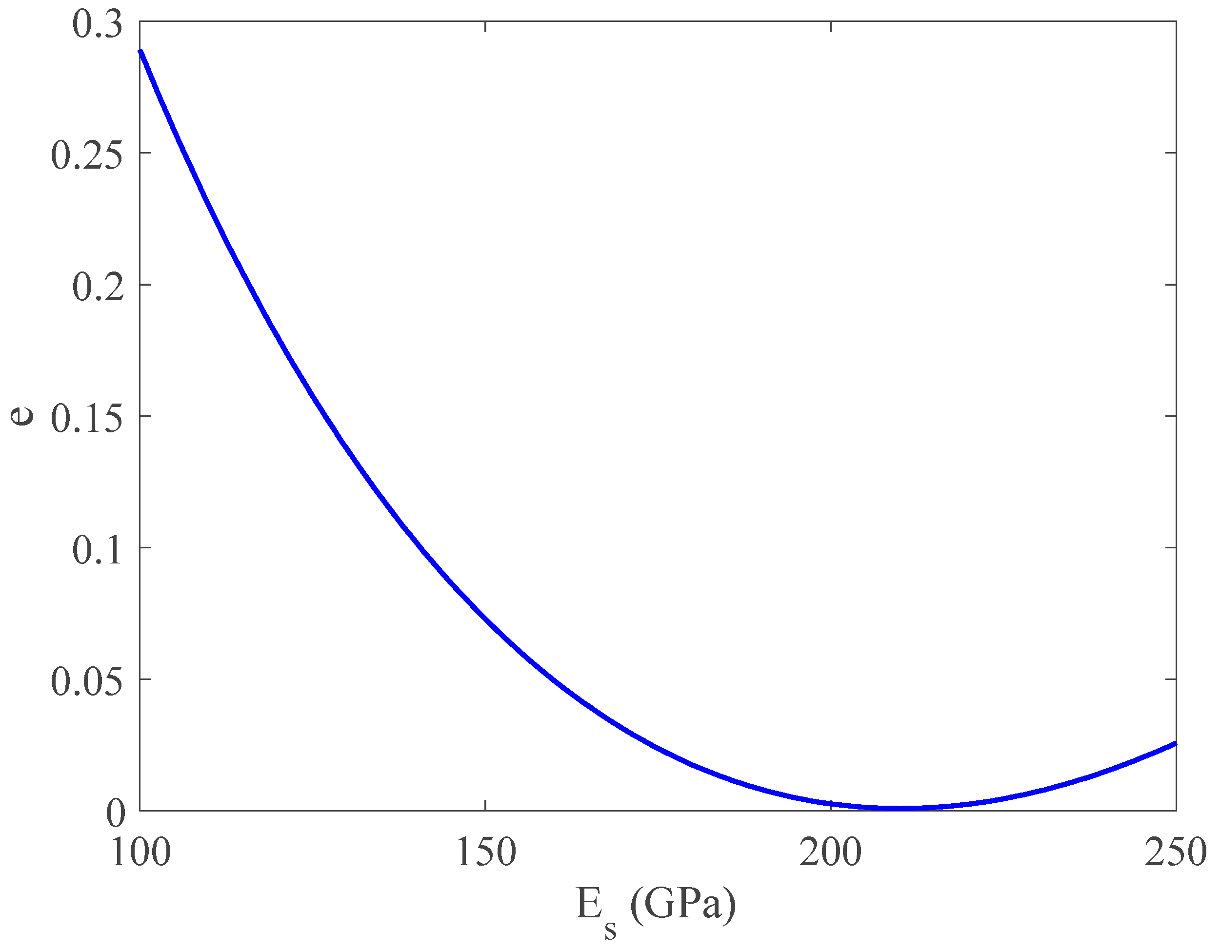
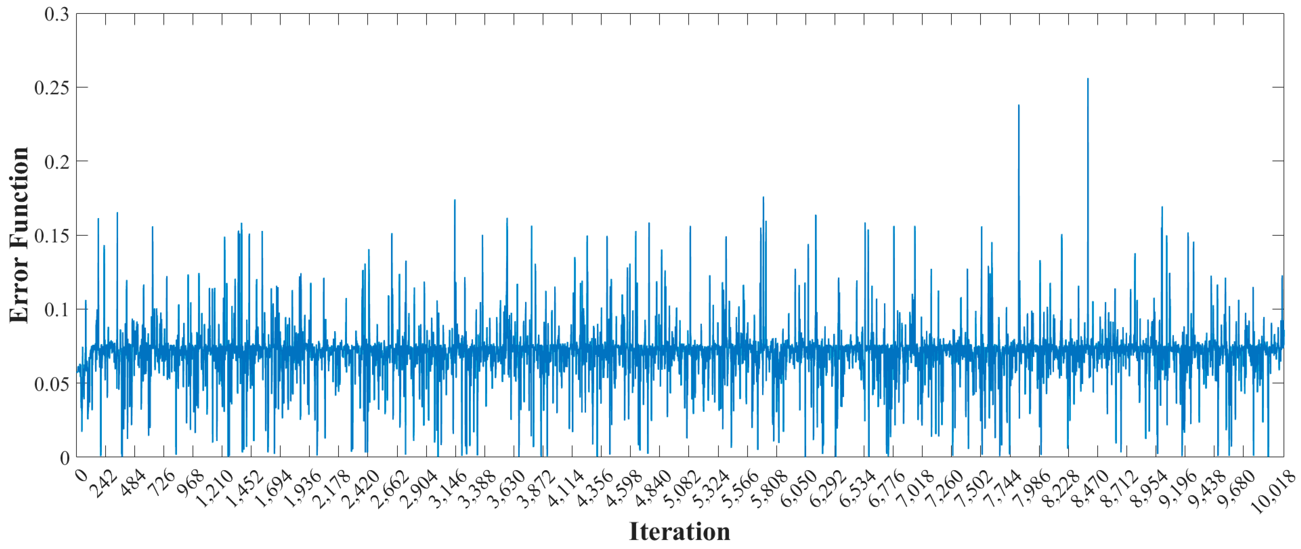
Thus, now it is possible to use the above mentioned experimental eigenfrequencies to set up an iterative procedure capable of finding the longitudinal elastic modulus value E_s:

• Select a value of E_s;
• Calculate theoretical eigenfrequencies using Equation (11);
• Estimate the quadratic error e of Equation (3) comparing experimental eigenfrequencies and theoretical ones.

The steps are repeated till a minimum value of error e is obtained. Figure 8 presents the trend of error function e that easily points at the optimal value of E_s-opt = 205 GPa. In this way, it was possible to have very little relative error (less than 1%) between the real E_s-real = 203 GPa and the ones that minimize the difference in the eigenfrequencies, see

Table 4. Comparison between experimental eigenfrequencies of the simply supported beam and the corresponding numerical ones with the optimal value of the longitudinal elastic modulus E = 205 GPa.

Mode	fi,s [Hz]	fi,n [Hz]	$\mathbf{\Delta }$ %
1	6.00	5.91	−1.55
2	23.23	22.48	−3.22
3	57.52	58.15	1.08
4	100.12	102.48	2.36
5	142.93	144.71	1.24

, confirming the accuracy of the developed approach. Thus, when measuring the experimental eigenfrequencies, it is possible to set up an inverse problem that can allow to determine the unknown mechanical characteristics.

This first application represents a validation for both the modal analysis and the parametric identification. Indeed, it was developed with known eigenfrequencies and material mechanical properties.

3.3.2. Cantilever Beam

The cantilever beam geometrical characteristics are different from those of the simply supported beam. Indeed, its density is 7652.02 kg/m³, the steel longitudinal elastic modulus E_s is still 203 GPa, while geometrical dimensions are L = 820.00 mm, b = 119.97 mm, and h = 10.08 mm. To create the full constraint, the beam was clamped for a length of 120 mm. Figure 9 presents the experimental set up for the cantilever beam, which shows the positions of the vibrodyne and of the accelerometer on the free side in order to avoid, once again, the nodes of the beam eigenmodes and maximize the vibration amplitude. The vibrodyne was still used while varying randomly the rotation speed (in order to mimic the white noise condition) and the test was repeated 6 times with a sampling frequency equal to 500 Hz.

For this case study, the first three flexural modal frequencies were considered. Figure 10 shows the considered beam eigenmode shapes, and

Table 5. Experimental eigenfrequencies of the cantilever beam and the corresponding standard deviation (SD).

Mode	fi,s [Hz]	SD [Hz]
1	11.41	0.17
2	86.68	0.01
3	257.26	0.35

shows the respective eigenfrequencies measured in the experimental tests.

In order to take into account the uncertainties due to the experimental constraint, a flexural spring $k_1$ and a translational one $k_2$ were introduced in the analytical model.

Given the position of the mass of the vibrodyne and the accelerometer in this experimental case, the Euler–Bernoulli beam Equation (7) was integrated while considering only one field with a lumped mass on the free end, see Figure 11.

Following what was performed in Section 3.3.1, the space variation of the solution is expressed by Equation (12):

$$v_j\left(x\right)=A_{1j}\mathit{cos}\left(\frac{{\lambda }_{j}x}{l}\right)+A_{2j}\mathit{sin}\left(\frac{{\lambda }_{j}x}{l}\right)+A_{3j}\mathit{cos}\mathit{h}\left(\frac{{\lambda }_{j}x}{l}\right)+A_{4j}\mathit{sin}\mathit{h}\left(\frac{{\lambda }_{j}x}{l}\right)$$

(12)

In this case, the four boundary conditions express the static and cinematic compatibility represented by Equation (10) already shown in Section 3.3.1.

Additionally, in this case, the frequency function was obtained by enforcing the singularity of the system matrix in Equation (10) by Equation (11). In this way, by enforcing Equation (11), it is possible to calculate the beam eigenfrequencies as a function of Young’s modulus $E_s$ and the constraint stiffnesses $k_1$ and $k_2$. Given its strongly implicit form, the roots of Equation (11) must be found with a numerical approach. In this case, again, the optimization procedure is based on minimizing the difference between the model eigenfrequencies (depending on $E_s$, $k_1$, $k_2$) and the experimental ones obtained by OMA. The optimization was performed by means of the simulated annealing algorithm.

For the described case of a cantilever beam, the minimum difference in eigenfrequencies (see

Table 6. Comparison between experimental eigenfrequencies of the cantilever beam and the corresponding numerical ones with the best value of the longitudinal elastic modulus E = 201 GPa.

Mode	fi,s [Hz]	fi,n [Hz]	$\mathbf{\Delta }$ %
1	11.41	11.62	1.86
2	86.68	85.59	−1.25
3	257.26	255.56	−0.66

) is reached for a value of the longitudinal elastic modulus equal to $E_s$ = 201 GPa and for values of the constraint stiffnesses equal, respectively, to $k_1=6.89\times {10}^{15} \mathrm{Nm}$ and $k_2=9.86\times {10}^{19} \raisebox{1ex}{$\mathrm{N}$}\!\left/ \!\raisebox{-1ex}{$\mathrm{m}$}\right.$.

In order to check the consistency of the obtained results, different optimizations were developed varying the initial ranges of the unknown parameters.

Table 7. Different variation ranges and optimal values of the unknown parameters for the cantilever beam case.

${\mathit{E}}_{\mathit{s}}$  [GPa] Init. Range	${\mathit{k}}_1$ [Nm] Init. Range	${\mathit{k}}_2$ [N/m] Init. Range	${\mathit{E}}_{\mathit{s}}$ [GPa]	${\mathit{k}}_1$ [Nm]	${\mathit{k}}_2$ [N/m]
1 $÷$ 210	1 $·$ 10−2 $÷$ 1 $·$ 1020	1 $·$ 10−2 $÷$ 1$·$ 1020	201.0	6.859 × 1017	9.720 × 1019
10 $÷$ 210	1 $·$ 10−2 $÷$ 1 $·$ 1020	1 $·$ 10−2 $÷$ 1 $·$ 1020	200.9	6.891 × 1015	9.971 × 1019
1 $÷$ 400	1 $·$ 10−2 $÷$ 1 $·$ 1020	1 $·$ 10−2 $÷$ 1 $·$ 1020	201.0	1.213 × 1016	9.967 × 1019
1 $÷$ 300	1 $·$ 10−2 $÷$ 1 $·$ 1020	1 $·$ 10−2 $÷$ 1 $·$ 1020	201.0	6.784 × 1015	9.700 × 1019
200 $÷$ 210	1 $·$ 1011 $÷$ 1 $·$ 1020	1 $·$ 1011 $÷$ 1 $·$ 1020	201.0	1.398 $·$ 1016	9.828 × 1019
1 $÷$ 400	1 $·$ 1010 $÷$ 1 $·$ 1020	1 $·$ 1010 $÷$ 1 $·$ 1020	201.0	1.214 $·$ 1016	9.487 × 1019

reports the main results showing a good consistency of $E_s$ and $k_2$, while the values of $k_1$ presents larger variation.

In addition, it is interesting to analyze the performance of the method when less eigenfrequencies are considered in the target function. For this reason, the optimization was performed considering just the first eigenfrequency, the first two eigenfrequencies, or all three eigenfrequencies.

Table 8. Different variation ranges and optimal values of the unknown parameters for the cantilever beam case. Optimal solution with different number of eigenfrequencies considered in the target function.

Considered Eigenfrequencies	${\mathit{E}}_{\mathit{s}}$ [GPa]	${\mathit{k}}_1$ [Nm]	${\mathit{k}}_2$ [N/m]
1	201.0	6.893 × 1015	9.781 × 1019
1–-2	201.0	1.662 × 1015	9.783 × 1019
1–2–3	201.0	1.213 × 1016	9.967 × 1019

reports the results of this analysis using as initial variation ranges: 1 $÷$ 400 GPa for $E_s$, 1 $·$ 10¹⁰ $÷$ 1 $·$ 10² Nm for $k_1$ and 1 $·$ 10¹⁰ $÷$ 1 $·$ 10²⁰ N/m for $k_2$. Looking at Table 8, it is quite clear how for the specific problem it is possible to reach a good estimation of the parameters while also considering just the first eigenmode. The information added from the second and third eigenfrequencies does not significantly change the solution.

3.3.3. Comparison to Other Optimization Algorithms

In order to test the efficiency of the proposed methodology based on the SA optimization algorithm, the same cantilever beam case was analyzed using two different heuristic algorithms: ant colony [19] and particle swarm [20].

The ant colony (AC) algorithm is a type of swarm intelligence algorithm inspired by the behavior of ant colonies. It is used to find the shortest path between two points in a graph. The algorithm simulates the behavior of ants as they search for food. In fact, each ant drops a pheromone trail as it traverses the graph, so that other ants are more likely to follow the paths with stronger pheromone trails. Over time, the pheromone trails will converge on the shortest path. The algorithm also includes a pheromone evaporation mechanism to prevent the trails from becoming too strong.

The particle swarm optimization (PS) algorithm is a type of optimization algorithm inspired by the behavior of bird flocks and fish schools. It is used to find the optimal solution of a problem by simulating the behavior of a group of particles, where each represents a possible solution. The particles move in the search space, guided by their current position and the best position encountered so far by any particle in the group (global best) and by the best position encountered by that particular particle (personal best). The movement of the particles is, therefore, determined by a combination of their velocity and acceleration, which are updated at each iteration based on the current global and individual best positions.

These algorithms have been implemented in Matlab^TM 2013 [36] and applied to the cantilever beam case in the model updating phase of the identification strategy, i.e., in the minimization of the difference between the model eigenfrequencies (depending on $E_s$, $k_1$, $k_2$) and the experimental ones obtained by OMA. This difference represents the target function to the minimization of $e$, see Equation (3).

All the algorithms were set up to use the following variables’ initial variation ranges: 1 $÷$ 4 $·$ 10² GPa for $E_s$, 1 $·$ 10⁻² $÷$ 1 $·$ 10⁻² Nm for $k_1$ and 1 $·$ 10⁻² $÷$ 1 $·$ 10²⁰ N/m for $k_2$.

The results of the optimization are shown in

Table 9. Performance of different optimization algorithms for the cantilever beam case.

Algorithm	e	${\mathit{E}}_{\mathit{s}}$ [GPa]	${\mathit{k}}_1$ [Nm]	${\mathit{k}}_2$ [N/m]
Simulated Annealing (SA)	0.023352	201.0	6.783 × 1015	9.867 × 1019
Ant Colony (AC)	0.028223	204.7	5.372 × 1019	7.082 × 1019
Particle Swarm (PS)	0.023353	201.0	4.451 × 1019	5.748 × 1019

where the error function value $e$, the elastic modulus E_s, the flexural spring $k_1$, and the translational one $k_2$ values are reported.

Looking at Table 9, it is clear that the minimum value of the error function was reached by the SA algorithm, while similar values of the elastic modulus $E_s$ and of translational spring $k_2$ were obtained by the three algorithms. However, largest differences have been found in the values of flexural spring $k_1$.

Looking at these results, the last case study presented in Section 3.4 was analyzed using the SA algorithm.

3.4. Steel Frame

The third experimental case is focused on a steel loading frame (Figure 12) located in the Materials Strength Laboratory of the University of Cagliari.

The frame is composed of two columns fully constrained at the base, connected by a cross beam hinged on the above-mentioned columns at adjustable heights. The latter connection is obtained with a pin, while at the columns base, welded and bolted connections ensure a full constraint for displacements, though small rotations are allowed. Thus, the rotation constraint can be represented by a set of flexural springs. The unknown parameters that are necessary for structural identification with the proposed methodology are the constraint rotational stiffnesses at the column bases.

All structural components are made of S275 steel grade, according to UNI EN 10025 [37], except for the pins, which are made of S355 steel grade. Each column is made of two 25 × 200 mm holed plates 40 mm apart, joined by 40 25 × 45 mm welded battens 250 mm apart and has a total height of 4965 mm. Fifteen holes with a diameter of 50 mm along each column allow the crossbar to be placed variably from a minimum height of 1105 mm to a maximum of 4605 mm. The crossbar consists of two L-shaped welded profiles made of two plates: 120 × 25 mm for the vertical leg and 325 × 25 mm for the horizontal one. The two angles are, thus, coupled by means of welded battens 420 mm apart. The beam has a total length of 5910 mm and can be employed at the maximum span of 5040 mm.

To determine the eigenfrequencies, five accelerometers were installed in the frame, three of which were mounted at one end of the beam and two at the top of the columns (Figure 13). The OMA yields the first 3 eigenfrequencies of the frame, once again determined by the peak picking method (see

Table 10. Experimental eigenfrequencies of the steel frame.

Mode	fi,s [Hz]
1	1.97
2	3.25
3	4.23

).

In this case, the frame model has been developed with finite element analysis (FE). In fact, the presented method is suitable for the update of a finite element model, aimed at the minimization of the difference between real modal parameters (e.g., eigenfrequencies) and the numerical ones. In this application, the stiffness k_ij of the springs representing the constraint conditions at the base of the column was chosen as the unknown parameter of the optimization process. For this purpose, a proper Fortran code was developed to call the finite element analysis execution for each iteration of the optimization procedure, along with the execution of the simulated annealing algorithm employing the numerical results.

The 3D finite element model was developed using the commercial software Strand7 (see Figure 14). For the modeling of the columns and the crossbeam, 15,948 four-node bilinear isoparametric plate elements were used. Mutual and base connections of steel members were modeled by means of multipoint constraints employing a total of 234 link elements. In detail, the pin connections were modeled as hinged internal constraints involving translational rigid links, while the base column connections were carried out by constraining the base section to a master node where flexural base springs were located. The examination of structural details suggested that no translations were likely to occur at the column bases, thus no translational base springs were taken into account. For the same reason, no torsional springs were accounted for. In both cases, the degrees of freedom were rigidly restrained. The total number of model nodes is 17,702.

This modeling strategy represents the best compromise between accuracy of results and computational efforts. The modulus of elasticity adopted for the material is E_s = 210,000 MPa and the specific weight is 7870 kg/m³.

Therefore, the optimization process was implemented with the aim of calibrating the stiffness of the flexural base springs, only one around x-axis k_x and the two flexural stiffnesses k_z1 and k_z2 around the z-axis, pertaining to the base master nodes. The choice of having two different flexural springs (k_z1 and k_z2) for rotations around the z-axes of each column and only one k_x stiffness for the rotations around x-axis, stemmed from evaluation of structural details and their effects on the measured eigenfrequencies.

The algorithm performed 10,018 iterations (Figure 15 and Figure 16), identifying at the iteration number 6047 the parameters that minimize the difference between the experimental and model eigenfrequencies, see Equation (3).

Table 11. Values of k_x, k_z1, and k_z2 that minimize the error function.

Flexural Stiffness	Value [kNmm/rad]
kx	$7.93\times {10}^7$
kz1	$1.63\times {10}^7$
kz2	$1.54\times {10}^6$

shows the values of k_x, k_z1, and k_z2 that make the error function equal to $4.83\times {10}^{-5}$, while the comparison between the experimental frequencies and the frequencies determined with the calibrated model is shown in

Table 12. Comparison between experimental eigenfrequencies of the steel frame and the corresponding numerical ones with the best value of the k_x, k_z1, and k_z2 [kNmm/rad].

Mode	fi,s [Hz]	fi,n [Hz]	Δ %
1	1.97	1.96	0.62
2	3.25	3.25	−0.05
3	4.23	4.24	−0.30

.

4. Discussion and Conclusions

This paper presented an innovative methodology for structural identification using OMA by the minimization of the difference between experimental and theoretical modal parameters, specifically the eigenfrequencies, using simulated annealing. Properly chosen unknown structural parameters are the variables of the minimization procedure that, by means of analytical or numerical models, allows to improve the knowledge of the structure with negligible damage to the structure itself and to its service. Indeed, OMA can be performed without any service interruption and allows to exploit environmental vibrations and service dynamic loads to evaluate experimental eigenfrequencies. The critical part of the methodology lies in the modeling and in the model optimization procedure used to tune the unknown parameters.

The method has been validated considering three new experimental cases: two small-scale steel beams and one full-scale steel frame. In the case of the simply supported beam, it was possible to assess the beam steel’s elastic modulus, while in the case of the cantilever beam, some constraint characteristics were evaluated as well. In the steel frame case, the focus was on the constraint conditions of the structure determining the flexural stiffness of the springs representing the column base constraints.

Section 3.3.3 presented a comparison between three different heuristic optimization algorithms: simulated annealing, ant colony, and particle swarm. Each algorithm was used to minimize the difference between the model eigenfrequencies (depending on structural mechanical parameters) and the experimental ones obtained using OMA. For the considered case, the SA algorithm obtained the best performance but good results were also obtained with the other two.

In the beam cases, the computational cost was very small and the code could yield the optimal solution in few seconds. A completely different situation was faced for the frame case. Indeed, each run of the finite element model required about 15 s, which needed to be repeated tens of thousands of times for the complete process, resulting in almost 2 days of computational time in a common PC equipped with 8 Gb of Ram and an intel i5 processor.

Another important aspect is the experimental eigenfrequencies identification. It is of paramount relevance to acquire and measure the highest number of eigenmodes and eigenfrequencies to improve the benchmark data necessary for parameter identification. In the considered cases, the eigenmodes of the beams were clearly detached and also the first modes of the frame were quite distant. This approach can be already developed in the case of close eigenmodes using more advanced techniques to analyze the accelerometer’s data.

In addition, it is not possible to find general relationships between the number of unknown parameters and the number of known eigenfrequencies considered in the target function that is always valid. Clearly, it is always better to have the largest amount of available information in the target function. The authors are persuaded that criticalities should be regarded in the general frame of ill-conditioned or rank deficient linear systems through spatial parameter estimation, see for example [38,39].

Finally, it is important to underline that the proposed case-studies are just examples for a general methodology that can be applied to larger structures where the values of elastic constants or constraint stiffness are not known or cannot be measured with simpler techniques. In particular, the estimation of constraint stiffness can be very important for existing steel structures where aging effects can modify the starting boundary conditions.

For this reason, further developments of this methodology are expected considering both damping property estimation and larger structures such as bridges or buildings that can represent interesting applications for this family of problems. The measurements of the modal parameters can be developed using also innovative techniques such as sound pressure as an excitation source and a laser doppler vibrometer as a sensor [10,11].

References

1. Stochino, F.; Fadda, M.L.; Mistretta, F. Low cost condition assessment method for existing RC bridges. Eng. Fail. Anal. 2018, 86, 56–71. [Google Scholar] [CrossRef]
2. Stochino, F.; Fadda, M.L.; Mistretta, F. Assessment of RC Bridges integrity by means of low-cost investigations. Frat. Ed Integrità Strutt. 2018, 46, 216–225. [Google Scholar] [CrossRef] [Green Version]
3. Franchi, A.; Napoli, P.; Crespi, P.; Giordano, N.; Zucca, M. Unloading and Reloading Process for the Earthquake Damage Repair of Ancient Masonry Columns: The Case of the Basilica di Collemaggio. Int. J. Archit. Herit. 2022, 16, 1683–1698. [Google Scholar] [CrossRef]
4. Zahid, F.B.; Ong, Z.C.; Khoo, S.Y. A review of operational modal analysis techniques for in-service modal identification. J. Braz. Soc. Mech. Sci. Eng. 2020, 42, 1–18. [Google Scholar] [CrossRef]
5. Bendat, J.; Piersol, A. Engineering Applications of Correlation and Spectral Analysis; Wiley: New York, NY, USA, 1993. [Google Scholar]
6. Felber, A.J. Development of a Hybrid Bridge Evaluation System; University of British Columbia: Vancouver, BC, Canada, 1994. [Google Scholar]
7. Brincker, R.; Zhang, L.; Andersen, P. Modal identification from ambient responses using frequency domain decomposition. In Proceedings of the 18th International Modal Analysis Conference (IMAC), San Antonio, TX, USA, 7–10 February 2000. [Google Scholar]
8. Kim, B.H.; Stubbs, N.; Park, T. A new method to extract modal parameters using output-only responses. J. Sound Vib. 2005, 282, 215–230. [Google Scholar] [CrossRef]
9. De Moor, B.; Van Overschee, P.; Suykens, J. Subspace algorithms for system identification and stochastic realization. In Proceedings of the MTNS, Kobe, Japan, 17–21 June 1991. [Google Scholar]
10. Scislo, L.; Guinchard, M. Non-invasive measurements of ultra-lightweight composite materials using Laser Doppler Vibrometry system. In Proceedings of the 26th International Congress on Sound and Vibration, ICSV, Montreal, QC, Canada, 7–11 July 2019. [Google Scholar]
11. Scislo, L. Quality Assurance and Control of Steel Blade Production Using Full Non-Contact Frequency Response Analysis and 3D Laser Doppler Scanning Vibrometry System. In Proceedings of the 11th IEEE International Conference on Intelligent Data Acquisition and Advanced Computing Systems: Technology and Applications, Cracow, Poland, 22–25 September 2021. [Google Scholar]
12. Yuan, K.; Zhu, W.D. Estimation of modal parameters of a beam under random excitation using a novel 3D continuously scanning laser Doppler vibrometer system and an extended demodulation method. Mech. Syst. Signal Process. 2021, 155, 107606. [Google Scholar] [CrossRef]
13. Kirkpatrick, S.G.C.; Al, E. Optimization by Simulated Annealing. Science 1983, 1, 671–680. [Google Scholar] [CrossRef]
14. Nikolaev, A.G.; Jacobson, S.H. Simulated Annealing; Gendreau, M., Potvin, J.Y., Eds.; Handbook of Metaheuristics; International Series in Operations Research & Management Science: New York, NY, USA, 2010; Volume 146. [Google Scholar]
15. Bertsimas, D.; Tsitsiklis, J. Simulated Annealing. Statist. Sci. 1993, 8, 10–15. [Google Scholar] [CrossRef]
16. Jenkins, W.M. Towards structural optimization via the genetic algorithm. Comput. Struct. 1991, 40, 1321–1327. [Google Scholar] [CrossRef]
17. Mei, L.; Wang, Q. Structural optimization in civil engineering: A literature review. Buildings 2021, 11, 66. [Google Scholar] [CrossRef]
18. Greco, R.; Vanzi, I. New few parameters differential evolution algorithm with application to structural identification. J. Traffic Transp. Eng. 2019, 6, 1–14. [Google Scholar] [CrossRef]
19. Angelo, J.S.; Bernardino, H.S.; Barbosa, H.J. Ant colony approaches for multiobjective structural optimization problems with a cardinality constraint. Adv. Eng. Softw. 2015, 80, 101–115. [Google Scholar] [CrossRef]
20. Poli, R.; Kennedy, J.; Blackwell, T. Particle swarm optimization. Swarm Intell. 2007, 1, 33–57. [Google Scholar] [CrossRef]
21. Sivori, D.; Lepidi, M.; Cattari, S. Structural identification of the dynamic behavior of floor diaphragms in existing buildings. Smart Struct. Syst. 2021, 27, 173–191. [Google Scholar]
22. Gesualdo, A.; Fortunato, A.; Penta, F.; Monaco, M. Structural identification of tall buildings: A reinforced concrete structure as a case study. Case Stud. Constr. Mater. 2021, 15, e00701. [Google Scholar] [CrossRef]
23. Lacanna, G.; Betti, M.; Ripepe, M.; Bartoli, G. Dynamic identification as a tool to constrain numerical models for structural analysis of historical buildings. Front. Built Environ. 2020, 6, 40. [Google Scholar] [CrossRef]
24. Şahin, A.; Bayraktar, A. Forced-Vibration Testing and Experimental Modal Analysis of a Steel Footbridge for Structural Identification. J. Test. Eval. 2014, 42, 695–712. [Google Scholar] [CrossRef]
25. Ren, W.X.; Zhao, T.; Harik, I.E. Experimental and analytical modal analysis of steel arch bridge. J. Struct. Eng. 2004, 130, 1022–1031. [Google Scholar] [CrossRef]
26. Rinaldi, C.; Ciambella, J.; Gattulli, V. Image-based operational modal analysis and damage detection validated in an instrumented small-scale steel frame structure. Mech. Syst. Signal Process. 2022, 168, 108640. [Google Scholar] [CrossRef]
27. Mousavi, A.A.; Zhang, C.; Masri, S.F.; Gholipour, G. Structural damage localization and quantification based on a CEEMDAN Hilbert transform neural network approach: A model steel truss bridge case study. Sensors 2020, 20, 1271. [Google Scholar] [CrossRef] [Green Version]
28. van Laarhoven, P.J.M.; Aarts, E.H.L. Simulated Annealing, Simulated Annealing: Theory and Applications; Mathematics and Its Applications, Springer: Dordrecht, The Netherlands, 1987; Volume 37. [Google Scholar]
29. Metropolis, N.R.A.; Al, E. Equation of state calculations by fast computing machines. J. Chem. Phys. 1953, 21, 1087–1092. [Google Scholar] [CrossRef] [Green Version]
30. Stochino, F.; Lopez Gayarre, F. Reinforced Concrete Slab Optimization with Simulated Annealing. Appl. Sci. 2019, 9, 3161. [Google Scholar] [CrossRef] [Green Version]
31. Oldenhuis, R.P. Trajectory Optimization for a Mission to the Solar Bow Shock and Minor Planets. Master’s Thesis, University of Delft, Delft, The Netherlands, 2010. [Google Scholar]
32. Welch, P. The use of fast Fourier transform for the estimation of power spectra: A method based on time averaging over short, modified periodograms. IEEE Trans. Audio Electroacoust. 1967, 15, 70–73. [Google Scholar] [CrossRef] [Green Version]
33. Gentile, C.; Saisi, A. Ambient vibration testing of historic masonry towers for structural identification and damage assessment. Constr. Build. Mater. 2007, 21, 1311–1321. [Google Scholar] [CrossRef]
34. Levin, R.I.; Lieven, N.A.J. Dynamic finite element model updating using simulated annealing and genetic algorithms. Mech. Syst. Signal Process. 1998, 12, 91–120. [Google Scholar] [CrossRef] [Green Version]
35. Frýba, L. Dynamics of Railway Bridges; Thomas Telford Ltd.: London, UK, 1996. [Google Scholar]
36. Math Works; MATLAB 2013.a Documentation: Natick, MA, USA, 2013.
37. CEN/TC 459/SC 3; 10025-Hot Rolled Products of Structural Steels Hot rolled Products of Structural Steels—Part 2: Technical Delivery Conditions for Non-Alloy Structural Steels. European Committee for Standardisation: Brussels, Belgium, 2019.
38. Mottershead, J.E.; Foster, C.D. On the treatment of ill-conditioning in spatial parameter estimation from measured vibration data. Mech. Syst. Signal Process. 1991, 5, 139–154. [Google Scholar] [CrossRef]
39. Mottershead, J.E.; Friswell, M.I. Model updating in structural dynamics: A survey. J. Sound Vib. 1993, 167, 347–375. [Google Scholar] [CrossRef]
Figure 1. (a) Data acquisition hardware Dymas 24. It is composed of 30 channels (1) managed by 5 acquisition cards (2), an internal battery, (3) and a central unit with CPU that has the task of managing the acquisition process, synchronization of the sensors, and data storage (4); (b) PCB 393 C accelerometer.
Buildings 13 00548 g001
Figure 2. Vibrodyne scheme.
Buildings 13 00548 g002
Figure 3. Steel beam geometrical characteristics.
Buildings 13 00548 g003
Figure 4. Simply supported beam experimental test scheme. The vibrodyne is on the left, while the accelerometer is on the right.
Buildings 13 00548 g004
Figure 5. First 5 beam eigenmode shapes.
Buildings 13 00548 g005
Figure 6. Internal forces acting on an infinitesimal Euler–Bernoulli beam.
Buildings 13 00548 g006
Figure 7. Integration field of the simply supported beam.
Buildings 13 00548 g007
Figure 8. Quadratic error e as a function of the elastic modulus for the simply supported beams.
Buildings 13 00548 g008
Figure 9. Cantilever beam experimental tests scheme. The vibrodyne is on the bottom while the accelerometer is on the top side of the free end.
Buildings 13 00548 g009
Figure 10. Considered eigenmode shapes for the cantilever beam.
Buildings 13 00548 g010
Figure 11. Cantilever beam analytical model.
Buildings 13 00548 g011
Figure 12. Steel frame picture (top) and geometrical dimensions (bottom), measures are in m.
Buildings 13 00548 g012aBuildings 13 00548 g012b
Figure 13. Detail of the positioning of the accelerometers at the end of the beam.
Buildings 13 00548 g013
Figure 14. Finite element model of the steel frame in the configuration adopted during the tests.
Buildings 13 00548 g014
Figure 15. Trend of the error function during the 10,018 iterations performed by the simulated annealing optimization algorithm varying kx, kz1, and kz2 parameters.
Buildings 13 00548 g015
Figure 16. Detail of the trend of the error function showing that the minimum was reached at iteration number 6047.
Buildings 13 00548 g016