Abstract
This study presents a two-step FE model updating approach for health monitoring and damage identification of prestressed concrete girder bridges. To reduce the effects of modeling error in the model updating process, in the first step, modal-based model updating is used to estimate linear model parameters mainly related to the stiffness of boundary conditions and material properties. In the second step, a time-domain model updating is carried out using acceleration data to refine parameters accounting for the nonlinear response behavior of the bridge. In this step, boundary conditions are fixed at their final estimates using modal-based model updating. To prevent the convergence of updating algorithm to local solutions, the initial estimates for nonlinear material properties are selected based on the first-step model updating results. To validate the applicability of the two-step FE model updating approach, a series of forced-vibration experiments are designed and carried out on a pair of full-scale decommissioned and deteriorated prestressed bridge I-girders. In the first step, parameters related to boundary conditions, including stiffness of supports and coupling beams, as well as material properties, including initial stiffness of concrete material, are estimated. In the second step, concrete compressive strength and damping properties are updated. The final estimates of the concrete compressive strength are used to infer the extent of damage in the girders. The obtained results agree with the literature regarding the extent of reduction in concrete compressive strength in deteriorated concrete structures.
1. Introduction
Bridges are vital components of the transportation infrastructure. The average age of in-service bridges in the United States is increasing, which necessitates methods and tools to inform decision making related to the maintenance and/or replacement of these structures [1,2]. Finite Element (FE) model updating methods have emerged as a venerable procedure for operational health monitoring and post-event structural damage identification [3,4,5,6,7,8,9,10,11,12,13,14,15,16,17]. In these methods, the initial/baseline FE model—developed using available as-built drawings—is updated using measured dynamic responses. During this process, uncertain model parameters—including material properties, damping parameters, boundary conditions, etc.—are calibrated/estimated. The deviation of final estimates of model parameters from their initial/baseline values reveals information regarding the location and extent of damage in the structure.
FE model updating approaches are mainly divided into two groups. The first group is modal-based model updating, wherein the initial FE model is updated to match the identified modal properties of the structure. In this method, the modal properties are first identified using modal identification methods (e.g., [18,19,20,21,22]). Then, the parameters characterizing the linear response behavior of the FE model are estimated to reduce the discrepancies between the identified and FE-predicted modal properties [3]. The accuracy of the identified modal signatures is controlled by the level of nonlinearity in the response behavior of structure, measurement noise, excitation frequency range, and sensor sparsity. The uncertainty in the identified modal properties propagates into the model updating process and is reflected in the final estimates of model parameters [23]. In addition, modal properties cannot be used to infer parameters characterizing the nonlinear material behavior. Consequently, the updated FE model may not be able to predict the dynamic response behavior of the structure correctly, especially when the structure is subjected to material nonlinearity. Although the estimated linear model parameters can be used for structural monitoring and damage identification [24], the application of modal-based model updating for damage identification of reinforced concrete bridges has been shown to be limited [25,26]. The second group of model updating approaches is referred to as time-domain model updating [17,27,28]. In this approach, the unknown model parameters characterizing linear and/or nonlinear response behavior of structure are updated to reduce the discrepancies between the measured and FE-predicted responses in time domain. In contrast to the modal-based model updating method, the measured dynamic responses of the structure are used directly for model updating in this approach. The direct application of dynamic responses in time-domain model updating eliminates the propagation of modal identification uncertainties into the model updating process.
Several studies in the literature (e.g., [10,23,29,30,31,32,33,34,35]) have focused on the system and damage identification of bridges subjected to ambient or traffic excitation (i.e., operational conditions) using modal-based model updating. The performance of these methods is mostly evaluated by comparing the identified and posterior FE-predicted modal signatures of the bridge. Studies in [36,37] showed that the accuracy of the updated model is highly sensitive to the selection of unknown model parameters. Moreover, [38] indicates that damage detection of bridges would depend on the proper simulation of boundary conditions. A two-step FE model updating process is suggested in this study to resolve modeling errors due to boundary conditions.
Using measurements other than modal properties for model updating and damage identification of bridges has attracted research interest recently. While static/pseudo-static responses (e.g., displacement measurements) have been used in previous studies for model updating [5,11,17,39,40,41,42], acceleration measurements have not been used directly for the purpose of model updating of bridges under operational conditions. It is worth noting that static/pseudo-static responses contain limited information regarding the dynamic behavior of the bridge compared to acceleration measurements. Therefore, acceleration measurements can be more informative about the uncertain model parameters compared to static/pseudo-static responses. The target in this study is to use both the modal properties and acceleration responses for model updating and damage diagnosis through a two-step FE model updating process.
Moreover, previous studies have shown that weak identifiability and mutual dependency between model parameters, modeling errors, as well as convergence of parameters to local solution may challenge the model updating process [4,43,44]. These challenges are exacerbated in a real-world application, especially in cases with large number of uncertain model parameters and/or improper selection of initial values for the uncertain model parameters.
To resolve the above-mentioned issues, this study presents a sequential combination of modal-based and time-domain model updating for operational health monitoring and damage identification of aged bridges using acceleration responses. In this procedure, first, a deterministic modal-based model updating is carried out to estimate the linear model parameters of a bridge. These model parameters are related to boundary conditions and material properties. Then, in order to refine the parameter estimation and account for the nonlinear response behavior of the bridge, a time-domain model updating is carried out. In this step, nonlinear material properties, as well as the damping energy-dissipation-related model parameters, are estimated while the linear-elastic model parameters are fixed at their final estimates obtained from the modal-based model updating. The final estimates of material properties are used to infer/quantify damage in the bridge.
In summary, the reasoning behind introducing the sequential combination of modal-based and time-domain model updating, which constitute the novelties of this work, can be summarized as follows.
- Unknown boundary conditions often challenge the application of time-domain model updating for bridges since the model parameters are often dependent on the boundary conditions. Here, the modal-based model updating is used to identify the boundary conditions first.
- The application of modal-based model updating for damage identification of bridges is limited. This is likely due to the uncertainties in the identified modal signatures that propagate through the parameter estimation process. Therefore, here, the estimation of model parameters for damage identification will be refined through a subsequent time-domain model updating.
- The dynamic measurements can provide more information about the uncertain material parameters compared to the static/pseudo-static responses. Hence, here, the acceleration measurements are used directly in the time-domain model updating.
- To improve the numerical stability and convergence of the model parameters the linear and nonlinear response behavior of the bridge are assimilated through the two-step model updating process.
To show the two-step FE model updating method and validate its applicability for damage identification in a real-world setting, a pair of full-scale precast prestressed bridge I-girders were used as testbed structures. These girders were in service from 1971 until 2009 before they were decommissioned and repurposed for research experiments [45]. A series of forced-vibration experiments were designed specifically for this study. The girders were subjected to sinusoidal force excitations, and their acceleration responses were measured at different locations. First, the collected acceleration responses are used to identify the modal signatures of the testbed structure. Then, the two-step FE model updating is carried out. In the first step, the initial FE model of girders is updated in the modal domain, and boundary conditions, including stiffness of supports and coupling beams, as well as material properties, including initial stiffness of concrete material, are estimated. The updated model is used as the prior model in the Bayesian model updating process to estimate concrete compressive strength and damping properties. Comparison between the posterior FE-predicted responses and field measurements shows a good agreement in the time domain. Moreover, the final estimates of concrete compressive strength result in a realistic damage identification/quantification for the girders. This process validates the applicability of the introduced two-step FE model updating approach for damage identification of bridge structures/components under operational conditions. While the input load used in this study varies from moving traffic load, this study proves the concept for future real-world application.
The paper is organized as follows. Section 2 is focused on test methodology and preliminary results including an introduction to the testbed structure and the experiments, modal identification, and development of the initial FE model. The two-step FE model updating method and the results are discussed in Section 3. Concluding remarks are provided in Section 4.
2. Material, Test Methodology, and Preliminary Results
In this section, first, a description of the field experiment including testbed structure, dynamic excitation system, wireless sensing network, and force-vibration tests is presented. Then, the modal identification process and corresponding results are shown in Section 2.2. Finally, the initial FE model is developed in Section 2.3.
2.1. Description of the Field Experiment
2.1.1. Testbed Structure
The testbed structure in this study includes two AASHTO precast prestressed bridge I-girders that were part of the Maryland 90 bridge. After decommissioning, the girders were salvaged and transferred to the Turner-Fairbank Highway Research Center (TFHRC) in McLean, VA, USA to be used as a research testbed [45,46]. The cross-section and elevation views of the girders are shown in Figure 1.
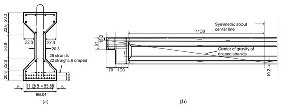
Figure 1.
The testbed structure: (a) cross-section view of each girder and (b) elevation view of each girder. All the dimensions are in centimeters, and all reinforcing rebars are #4 (equivalent to Φ13).
The studied girders are 1.37 m deep and 26 m long. Reinforcements and prestressing steel strands are shown in Figure 1. A side view of the testbed structure (with a 20 cm slab on top of each girder) is shown in Figure 2a. After being transferred to the TFHRC, each girder was placed on two 1 1 bearing pads on top of two 2.3 1.6 1.6 geosynthetic reinforced soil (GRS) piers [47]. These can be seen in Figure 2b,c. The girders were placed parallel to each other with 2.9 m centerline spacing and were connected with four coupling beams with 0.3 1.4 cross-sectional area. Three out of four coupling beams are seeable in Figure 2d.
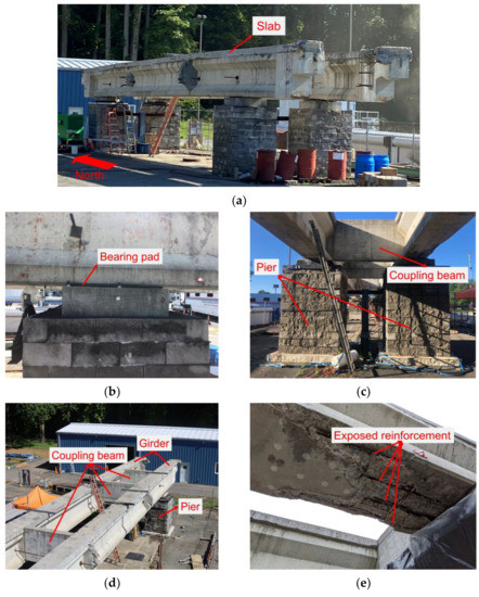
Figure 2.
Testbed structure: (a) side view and north direction, (b) bearing pad, (c) piers and coupling beam, (d) top view, and (e) example of existing damage (west girder close to the north pier).
The studied girders were in service in a corrosive environment for almost 40 years. The environment simultaneously exposed the concrete matrix of the girders to physical and chemical deterioration processes. Concrete delamination and degradation, as well as steel corrosion, are the main damage mechanisms for concrete bridges in such environment [48]. Due to this, the girders experienced aging and deterioration in several locations, including cracking, steel reinforcement corrosion, spalling, etc. Figure 2e shows an example of the observed damage in girders.
Aside from the aging-related damage discussed above, in 2012, salt spray chambers were installed on each girder to accelerate deterioration in the girders. The chamber installed on the west girder sprayed a 15 weight percent (wt.%) NaCl solution and the chamber installed on the east girder sprayed a 3.5 wt.% NaCl solution. This was part of a study to develop protocols for non-destructive testing (NDT) methods for prestressed girder bridges [45].
2.1.2. Dynamic Excitation System
The shaker used in this study was a small uniaxial hydraulic device capable of producing arbitrary displacement motions in the vertical direction. The device consisted of a hydraulic piston connected to a servo-hydraulic valve that controlled the motion of a stack of steel plates that combined to form 4450 N of moving weight. The motion was controlled by an MTS PID hydraulic controller using an LVDT sensor to provide feedback displacement. The shaker’s hydraulic piston, moving weights, and steel frame of the shaker were supported on four 4450 N load cells, which were used to measure the total force generated by the shaker. The load cells were installed between the shaker plate and the clamping plate on the girder. The shaker plate with dimensions of 30 cm 30 cm 2 cm was located on the top center of the clamping plate with dimensions of 140 cm 70 cm 5 cm (see Figure 3). The shaker displacement and force time histories were collected through a LORD-Microstrain V-Link-200 wireless node [49]. The wireless sensing network is discussed further in the following section. Figure 3 shows a close view of the shaker, and Figure 4 shows the two locations (layout 1 and layout 2) at which the shaker was installed on the testbed structure. The hydraulic power for the shaker was provided by a diesel-powered mobile pump.
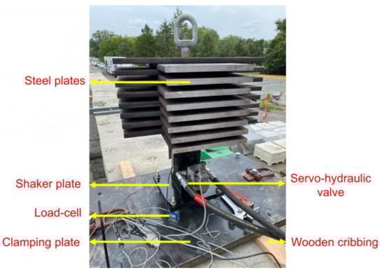
Figure 3.
The shaker installed on the girder.
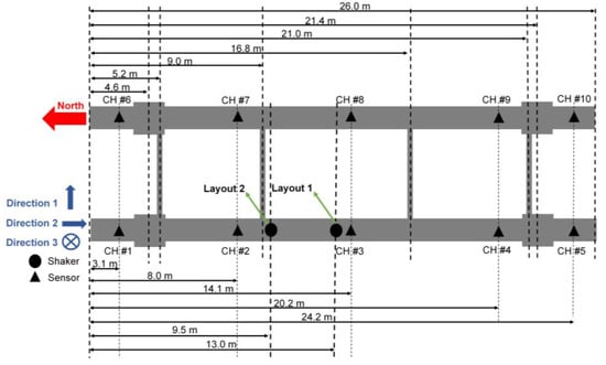
Figure 4.
Test layout including the sensor and shaker locations.
2.1.3. Wireless Sensing Network
The wireless sensing network included ten battery-powered triaxial MEMS wireless accelerometers (LORD-Microstrain G-Link-200) and a V-Link-200 node [49]. Each accelerometer had an adjustable measurement range of 8 g and could be configured for continuous, periodic, or event-triggered sampling modes to output acceleration, tilt, or derived vibration parameters (velocity, amplitude, etc.). The measured data could be transmitted in real-time and/or be saved to the onboard memory with storage capacity up to data points. The accelerometers had a noise density of 25 with a wireless range of up to 1 km and an adjustable sampling rate of up to 4 kHz. Each accelerometer had dimensions of 47 mm 43 mm 44 mm. To install the accelerometers, zinc-plated steel washers were glued on top surface of the girders. Then, each accelerometer was screwed to a magnetic base and attached to the washers. Figure 5 shows an installed wireless accelerometer. Data collection and coordination between the wireless nodes including the accelerometers and the V-Link-200 node, which was used to collect shaker data, were carried out through the wireless USB data acquisition gateway. The gateway used the lossless extended range synchronized (LXRS) data communication protocol and facilitated lossless data collection with node synchronization of 50 . Synchronization was carried out by transmission of a continuous system-wide timing reference known as the beacon. The communication between the gateway and sensors was wireless through a license-free 2.405 GHz to 2.480 GHz radio frequency with 16 channels. The configuration of the network, data acquisition initialization, and sampling mode selection were managed through the SensorConnect software [50], which was installed on a host computer. The layout of the employed accelerometers is shown in Figure 4. In this study, the sampling rate was 128 Hz, and the acceleration data were collected in directions 1 (i.e., east-west) and 3 (i.e., up-down).
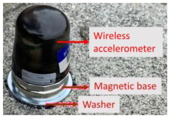
Figure 5.
A wireless accelerometer installed on the girder’s top surface.
2.1.4. Forced-Vibration Testing
The testbed structure was subjected to a series of designed sinusoidal force excitations through frequency sweeps with pre-defined frequency range, duration, and amplitude. Sweeps ranged between 2 Hz and 20 Hz, including 50 different frequencies increasing logarithmically with a duration of 30 s for each frequency. Moreover, the sweeps excited the girders with three different target load amplitudes equal to 445 N, 2225 N, and 4450 N. Considering two layouts (see Figure 4) and three levels of load amplitudes, girders were tested under six frequency sweeps. A general view of the testbed structure during the field experiments is shown in Figure 6. The excitation force time history and instantaneous excitation frequency—calculated using a short-time Fourier transform [51]—for each sweep are presented in Figure 7.
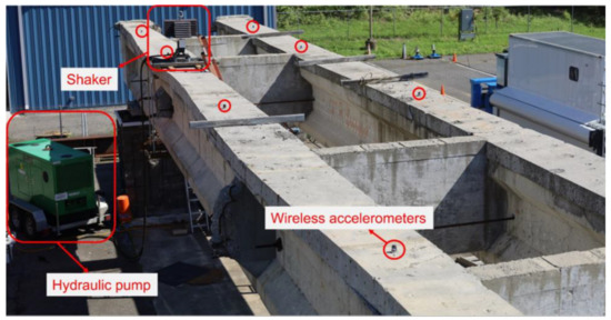
Figure 6.
The field experiment setup corresponding to layout 2 (See Figure 4).
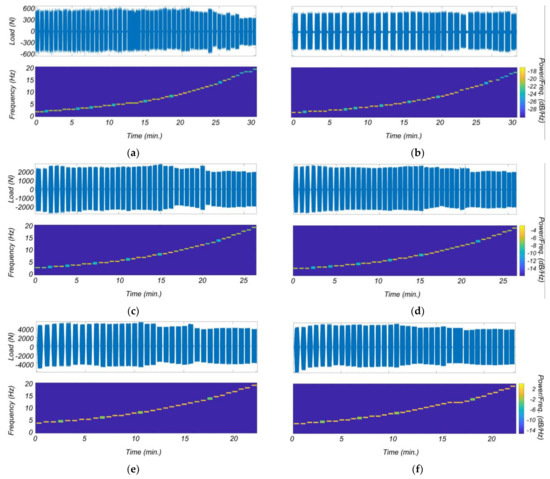
Figure 7.
Excitation force time histories and instantaneous excitation frequencies: (a) Layout 1 with 445 N target load amplitude, (b) Layout 2 with 445 N target load amplitude, (c) Layout 1 with 2225 N target load amplitude, (d) Layout 2 with 2225 N target load amplitude, (e) Layout 1 with 4450 N target load amplitude, and (f) Layout 2 with 4450 N target load amplitude.
2.2. Modal Identification
In this section, the modal properties of the testbed structure are identified from the forced-vibration experimental data. For the purpose of modal identification, the collected data from the sweep with layout 1 and 445 N target load amplitude are used (see Figure 7a). These data include the acceleration of 10 channels in directions 1 and 3 (results in 20 input signals—see Figure 4) and the shaker excitation force. A brief summary of the modal identification process and the identified modal properties are presented in this section.
Various modal identification techniques are available in the literature to identify modal properties—including natural frequencies, damping ratios, and mode shapes—from experimental data [19,21,22]. In this study, due to the nature of the excitation, the empirical frequency response functions (EFRFs) [22] are calculated using applied input (shaker excitation force) and measured outputs (acceleration responses). Then, the calculated multi-output EFRFs are used to estimate a state-space model. This two-stage frequency-domain approach helps to specify the frequency band of interest in which the modal identification needs to be carried out.
The EFRF between a measurement signal and input signal —depicted by —is defined as below:
where and are Fourier transforms of and , respectively. In a real-world setting, data are always polluted with measurement noise. To reduce the effects of the measurement noise and obtain a smooth EFRF, Welch’s averaging method [52] with 12,800 data points Hamming window is used for spectral estimation. This size of window is selected to ensure covering the full length of excitation and the ambient signal before and/or after it.
Having EFRFs for all 20 signals, an -order state-space model is estimated to fit the estimated EFRFs in the frequency band of interest. In this study, to reduce uncertainties due to low- and high-frequency noises, the frequency band of interest is selected between 2 to 25 Hz. Blue curves in Figure 8 show the calculated EFRFs using measured data.
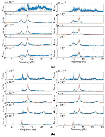
Figure 8.
EFRFs calculated from the experimental data (blue) and EFRFs estimated using the identified state-space model (red): (a) Direction 3 and (b) Direction 1.
To estimate the state-space model, the subspace state-space identification method is used [53,54]. While this method is briefly explained here, the proof of theory and more details can be found in [53]. In the subspace state-space identification method, measurements are placed in a block Hankel matrix which is divided into a past and a future part. The identification algorithm proceeds with projecting the future measurements into the past measurements, while the projection matrix can be factorized as the product of an observability matrix and a state sequence. These two matrices are identified by applying the singular value decomposition (SVD) to the projection matrix, and the order of the system is calculated as the number of non-zero singular values. By applying one block shift in separation between past and future measurements in the Hankel matrix, another projection matrix, shifted observability, and state sequence matrices can be obtained. At this point, the system matrices can be calculated from the overdetermined set of linear equations.
The numerical algorithms for system identifications are available in the Matlab n4sid [55] function and are used in this study. As a classical remedy, the modal identification is carried out for a range of model orders, and a stability diagram is plotted on which true modes appear as stable modes [56]. For this purpose, the stability analysis is run considering model orders from 2 to 40 with 1% and 5% error tolerances for natural frequency and damping ratios, respectively. The stability analysis showed that a model order of n = 26 is the lowest model order to have all stable modes within the frequency band of interest. The fits between estimated and calculated EFRFs can be improved using the prediction error minimization algorithm and nonlinear least-squares objective functions. This approach is carried out using the Matlab ssest function [57], which initializes the model parameters based on the previously estimated state-space model, and then updates the parameters using an iterative search to minimize the prediction errors [21]. Red curves in Figure 8 display EFRFs of the estimated state-space model at measurement points. As can be seen, the estimated state-space model is able to approximate the calculated EFRFs acceptably. Identified natural frequencies () and damping ratios () of the system are reported in Table 1. The identified mode shapes—those which will be used for modal-based model updating—are later shown in Section 3.1.

Table 1.
Identified natural frequencies and damping ratios.
2.3. Finite Element Modeling of the Testbed Structure
The initial FE model of the testbed structure is developed in OpenSees [58] using the available as-built drawings. The girders are modeled using fiber-section force-based beam-column elements (forceBeamColumn) with approximately 30 cm length and 3 integration points. Moreover, the linear-elastic shear stiffness and torsional stiffness are aggregated to the fiber sections. The slab is also modeled using rectangular fiber sections as a part of the girders’ sections. Steel reinforcement is modeled using single fibers located at the center of each bar. To model the profile of the draped strands—with a nominal cross-sectional area of 1 —the strands’ depth at the integration points of each element is calculated based on Figure 1. The strand is modeled using a single fiber at its corresponding depth. Concrete material for girders and slabs is modeled with nominal compressive strength ( and for the east and west girders) of 46 MPa, strain at maximum strength () of 0.2%, strain at crushing strength () of 0.5%, and zero crushing strength. As girders are already damaged, no tensile strength is assumed, and therefore, the Concrete01 material model is employed. To model the shear and torsional stiffness of the girder sections, the shear modulus (G) is calculated based on the concrete modulus of elasticity, (= ), and Poisson’s ratio of 0.2. Moreover, the shear area for girder sections is set equal to 0.38 and 0.65 in the Y and X directions (see Figure 1), and torsional constant of girder sections is set equal to 0.03 . The parameters and —modulus of elasticity for the east and west girders—are set equal to the initial slope in Concrete01 model (i.e., and ) which is 46 GPa here. Steel is modeled using bilinear steel01 material with a modulus of elasticity of 200 GPa, and yielding strength of 455 MPa and 1720 MPa for reinforcing steels and strands, respectively. Moreover, the prestressing force in strands (128.60 kN per strand) is modeled by applying its resulting initial strain to the steel material. For this purpose, the normal strain in strands’ steel resulting from the prestressing force is calculated by dividing the prestressing force by strand’s axial rigidity (product of the strand’s modulus of elasticity and gross section area). The calculated strain (0.65%) is assigned to the strands’ steel01 material using InitStrainMaterial. The mass, kg in total, and weight of the girders are assigned to the element nodes.
Coupling beams are modeled using elasticBeamColumn elements considering the gross cross-sectional area and an Elastic material with the modulus of elasticity equal to 30 GPa. The coupling beams are connected to the girders assuming rigid connections. The mass and weight of the coupling beams are assigned to the element nodes. To model each support, the girder nodes that are located along the bearing pad are constrained to a node at the center of the bearing pad using rigidLink constraint. To account for flexibility in the piers and bearing pads, supports are defined using a 6 degrees of freedom (DOFs) spring. This is modeled using ZeroLength elements with Elastic uniaxial material. Moreover, the energy dissipation in the piers and bearing pads is collectively modeled using a dashpot in the vertical direction. This is performed using ZeroLength elements with Viscous uniaxial material. The corresponding stiffness and damping parameters are initially selected based on engineering judgment [47,59] and are later updated using modal-based and time-domain model updating. In summary, the FE model consists of 214 beam-column elements, 16 rigidLink elements, 12 ZeroLength elements, and 230 joints. The list of model parameters that are later treated as unknown parameters in Section 3.1 and 3.2 and their initial values are summarized in Table 2. In this table, the equivalent values for concrete compressive strength and modulus of elasticities of girders are shown in the same row separated with ‘/’. The directions in this table are based on Figure 4.
Table 2.
Model parameters for the initial FE model. The directions in this table are based on Figure 4.
The nonlinear time history analysis is performed using the Newmark average acceleration method with a constant time step size of 0.0078 s equal to the measurement sampling rate. The Newton-Raphson method is used to iteratively solve the nonlinear equilibrium equations [60]. To define energy dissipation in the structural system aside from the material nonlinearity, modal damping is modeled for the first six modes. The damping ratios, i.e., , are set equal to the identified ones (see Table 1). The only exceptions are damping ratios for modes 1 and 2, which are set equal to 0.02. The reason is to have similar initial values—which is not very different from the identified values (0.0192 and 0.0178)—during time-domain model updating, which is discussed later.
3. Two-Step Model Updating: Methodology, Results, and Discussion
3.1. First Step: Modal-Based Model Updating
The modal properties of the initial FE model are different from the identified ones (Figure 9). Hence, the initial FE model needs to be updated using modal-based model updating to better fit the identified modal properties. As mentioned before, the modal-based model updating is limited to the linear response behavior of structures. Hence, only the linear model parameters are updated at this step. Modal-based model updating process is discussed next.
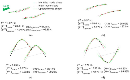
Figure 9.
Comparison between identified, initial, and updated modal properties: (a) first lateral mode, (b) second lateral mode, (c) first vertical mode, and (d) second vertical mode.
The modal-based model updating is a process to minimize the discrepancies between identified and FE-predicted modal frequencies and mode shapes by updating the linear parameters of the FE model [24,61]. In this process, an objective function, , is defined as shown in Equation (2). The discrepancies between modal frequencies, mode shapes, and a regularization term are respectively the first, second, and third terms in Equation (2).
In Equation (2), the parameter is the weighing scalar for frequency residuals and the term is the vector including the square root of normalized differences between FE-predicted and identified modal frequencies. The parameter is the weighing scalar for modal assurance criteria (MAC) residuals. The term N is the total number of identified modes that are used for model updating, and the term indicates the MAC value for mode . The parameter is the weighing scalar for penalizing large deviation of the unknown FE model parameters from their initial values. The vector is the vector of unknown FE model parameters and is the number of unknown model parameters for modal-based model updating. The vector is the initial estimates of the unknown model parameters. The entry of the vector , denoted as , is defined as follows:
In the above equation, the terms and are the modal frequencies of the identified and FE-predicted modes. The term is defined as follows:
The terms and are the identified and FE-predicted mode shape vectors, respectively, and NDOF is the number of DOFs. The superscript T denotes matrix/vector transpose operator.
To update the FE model using modal-based model updating, the stiffness-related model parameters (= = ), , , and are selected as unknown FE model parameters to be updated ( 5). Note that parameter is not selected as there is no measurement in the longitudinal direction of the girders. The vector is initiated using the initial values listed in Table 2.
The first two lateral and the first two vertical identified modes ( 4) are used for the modal-based model updating. This is because the first two identified vertical modes are the only ones with frequencies less than 20 Hz (maximum excitation frequency). As can be seen in Figure 4, measurements are collected in 5 vertical (i.e., in direction 3) and 5 lateral (i.e., in direction 1) DOFs for each girder; therefore, = 20. The terms , and are selected equal to 4, 1, and 0.01 to balance the contributions of the MAC value and frequency errors in the objective function. As a result, the difference between identified and estimated modal frequencies will be penalized more than mode shapes [61]. This is because the uncertainty in identified mode shapes is greater than frequencies. The constrained nonlinear multivariate optimization function fmincon within the Matlab Optimization Toolbox is used [62] with the interior-point algorithm [63]. The maximum iteration number is set to 30, and the process terminates when the relative difference between successive values of the objective function is lower than a given threshold of . Moreover, the lower and upper bounds for parameter estimation are set equal to times of the initial values.
A comparison between the identified, initial, and updated modal properties is shown in Figure 9, and the updated values for the FE model parameters are shown in Table 3. It is noteworthy that as parameters = are updated, the parameters are also updated (using and assuming fixed value for ). These equivalent values for each girder are shown in a same column in Table 3 and are separated using ‘/’. A comparison between Table 2 and Table 3 shows that the parameters and are estimated to a smaller value than their initial ones. This was expected as both girders are aged and have experienced severe damage. The parameter is estimated to a smaller value than its initial one. This is probably due to the presence of cracks in the section and could also be an indication of the fact that the connections between the girders and coupling beams are not completely rigid. The parameters , and are estimated to have values greater than their initial ones, which indicates that the bearing pads are stiffer than what is considered in the initial model. The improvement in the modal frequencies is superior to the MAC values. This means that the modal-based model updating process compensates for the frequency match with MAC values. The maximum error in frequency is at the second lateral mode, which is less than 8% and is acceptable. The updated model is later used as the prior FE model for the time-domain model updating.
Table 3.
The updated FE model parameters after modal-based model updating.
3.2. Second Step: Time-Domain Model Updating
To this point, the initial FE model of the studied girders is updated using modal-based model updating. It is noteworthy that concrete material has nonlinear response behavior even under small levels of excitation. In addition to that, presence of prestressing force pushes the concrete material across the section along its nonlinear response curve. Then, the applied excitation—shaker force here and traffic load in operational conditions—results in small loading/unloading of concrete material in nonlinear range of the response curve. The level of nonlinearity in the response behavior of concrete material increases as a function of deterioration and damage [64]. However, the nonlinear response behavior of the studied girders is not captured through modal-based model updating.
To account for the nonlinear response behavior of girders as well as refining the estimation of damage-related model parameters, time-domain model updating—here referred to as the second step of the model updating procedure—is carried out. The cumulative damage effects in a reinforced concrete section can be modeled by altering the stress-strain response behavior of the concrete material, e.g., reduction of the effective compressive strength [65,66,67]. Based on this, it is intended to estimate the concrete compressive strengths of girders using time-domain model updating. Moreover, the acceleration measurements contain information regarding the dynamic behavior of the testbed structure. Hence, the energy-dissipation-related model parameters can also be estimated using time-domain model updating. For this purpose, first, the most identifiable FE model parameters are selected using an information-theoretic identifiability analysis [68]. Then, these parameters are updated using the Bayesian model updating process.
3.2.1. Identifiability Analysis for Time-Domain Model Updating
The identifiability analysis is an approach to determine the most identifiable unknown model parameters using the sensitivity of FE-predicted responses with respect to the unknown model parameters. In this method, the relative information that each candidate model parameter gains from the responses and the mutual information gain between these parameters are calculated. The model parameters with high relative information gain and little dependency on other parameters are likely more identifiable than others and are selected to be updated in the model updating process.
The data used for identifiability analysis are noted as Data 1-2 in Table 4, which corresponds to layout 1 and the target load amplitude of 2225 N. It is noteworthy that no significant difference is expected in the identifiability analysis results using different layouts and target load amplitudes. However, the target load amplitude for identifiability analysis is selected high enough to have a moderate level of loading/unloading response behavior in the concrete material of the testbed structure. The data in Table 4 are later used for model updating.
Table 4.
Field experimental data used for the Bayesian FE mode updating. The measured data with excitation frequencies close to mode 1 and mode 2 are lumped together.
As can be seen in Table 4, the identifiability analysis and model updating process are performed using experiments with excitation frequencies of 9.73 Hz and 12.86 Hz. These excitation frequencies are selected as they are the closest ones to the identified modal frequencies (9.73 Hz and 12.79 Hz) and are expected to provide useful information on the dynamic behavior of the testbed structure. Moreover, the measured signal-to-noise ratio in the experiments with these frequencies is higher than the similar ratio in experiments with excitation frequencies far from the identified modal frequencies. A higher measured signal-to-noise ratio results in more stable parameter estimation [69].
Each data set in Table 4 augments two experiments with excitation frequencies of 9.73 Hz and 12.86 Hz (while the layout and target load amplitude are similar). This is shown in the following equations:
The terms and denote the acceleration measurements and input excitations that are being used for identifiability analysis and time-domain model updating. The terms and refer to the collected acceleration measurements (at 10 measurement channels in direction 3) from experiments with input excitation frequencies of 9.73 Hz and 12.86 Hz. The terms and refer to the input excitations with frequencies of 9.73 Hz and 12.86 Hz. The term is the total length of collected data.
One of the intentions of identifiability analysis/time-domain model updating is to analyze the identifiability of/update the unknown model parameters and . For this purpose, it is required to implement measurements from both excitation frequencies equal to 9.73 Hz and 12.86 Hz. The augmenting process provides measurements that contain dynamic response behavior of the testbed from both its vertical modes.
Parameters , , , , , , , and are selected as candidate unknown model parameters. It is intended to refine the damage state estimation of girders for the west and east girder separately. Therefore, the concrete compressive strengths of the west and east girders are modeled using two different parameters and , respectively. While the main intention of the time-domain model updating is to update the model parameters related to the energy dissipation and nonlinear behavior of the structure, the parameters , , and are also considered as candidate unknown parameters. As will be seen later, this is to highlight how the introduced two-step model updating helps with unidentifiability and mutual dependencies between the model parameters. Since the input load mainly excites the first two vertical modes of the girders, the modal damping ratios of these two modes are included in the list of candidates for unknown parameters. The value for parameters , , , , and are set equal to their final estimates in modal-based model updating (see Table 3). As the input load is in the vertical direction, the parameter is most probably not identifiable and is excluded from the list of candidate model parameters. The value of parameter is set equal to the updated value of (after modal-based model updating) as the properties of bearing pads are assumed to be the same in the transverse and longitudinal directions. The value of parameters , and are set equal to their initial values (see Table 2), as these parameters were not updated using modal-based model updating.
The relative information gain of the candidate unknown model parameters and relative mutual information gain between the candidate unknown model parameter pairs are shown in Figure 10. As can be seen in this figure, although the parameters , , , and have considerable levels of relative information gain, they are highly dependent on the parameters and . This dependency is likely because all these parameters contribute to the stiffness of the testbed structure. Based on this, parameters , , , and are most probably not identifiable together with parameters and . Parameters , , and reflects the linear-elastic response behavior of the testbed structure and are already estimated using modal signatures. Moreover, the parameters and have relatively large information gain, and their estimation is of main interest in time-domain model updating as their final estimates help to refine the damage estimation in girder level and reflect the cumulative damage status of each girder. Hence, parameters and are selected to be estimated using time-domain model updating while parameters , , and are fixed at their corresponding values in Table 3 obtained from the modal-based model updating. This reduces the challenges of model updating due to the unidentifiability and/or mutual dependencies between model parameters. It is noteworthy that the final estimates of parameters and using time-domain model updating will inherently be dependent on the fixed values selected for parameters , , , and . Parameters , , and have relatively moderate information gain and have a negligible dependency on other parameters. However, parameter is dependent on parameters and as all of them contribute to the viscous damping energy dissipation of the structure. As the initial value for parameter is selected based on judgment, it is of interest to update this parameter using the model updating process. However, the final estimates of parameters , and are expected to vary between different case studies and depend on each other. Therefore, the overall damping of the testbed will be calculated at the end. Based on the above discussion, parameters , , , , and are selected to be estimated using the time-domain model updating.
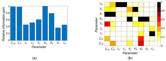
Figure 10.
Identifiability analysis results: (a) relative information gain of the candidate unknown model parameters; (b) relative mutual information gain between the candidate unknown model parameter pairs. Each row is normalized to its diagonal value. Then, the diagonal values are nullified.
3.2.2. Bayesian Inference
In the Bayesian model updating, the unknown FE model parameter vector is considered as a random vector with joint probability density function (PDF) whose mean (referred to as estimate hereafter) and covariance are updated recursively through the integration of the FE-predicted and measured responses. The unknown FE model parameters are updated using measured responses in successive overlapping windows. In this approach, known as the sequential estimation window approach [70], the a priori estimates of the unknown FE model parameters at each estimation window are updated to the a posteriori estimates. A brief review of this method is provided in the following.
Assuming zero-mean Gaussian white noise processes for the measurement noise () and the process noise (), the state-space model at each estimation window is set up as follows:
As can be seen in Equation (7), the unknown FE model parameter vector for Bayesian model updating, , evolves linearly in the state equation by a random walk process. The term is the number of unknown FE model parameters in the Bayesian model updating. In this study, the term is equal to 5 (which counts the number of parameters , , , , and ) and the initial values for the unknown model parameters are equal to those described in the previous section. In Equation (8), the term denotes the measurement vector and denotes the nonlinear FE-predicted response function at the estimation window, which spans between time steps and with time steps overlap with the previous estimation window. The parameter (here 20) is the number of collected signals and is number of time steps at the estimation window. The term is the deterministic input vector at the estimation window. In this study, estimation windows have the length of 150 time steps with 50 time steps overlap, i.e., 50 and 150 and 50 .
The measurement equation (Equation (8)) is linearized using the first-order Taylor series expansion with linearization point at the a priori estimate. The following equation is obtained:
in which the superscripts –/+ denote the a priori/posteriori estimates, and derivation of with respect to is referred to as the sensitivity matrix and is calculated using the finite difference approach. The estimation method that is used in this study is referred to as the Extended Kalman filter (EKF) for parameter-only estimation [71]. In this method, the a priori estimates of the mean vector and covariance matrix of the unknown model parameters at each estimation window are considered equal to the a posteriori estimates at the previous estimation window. This is depicted in Equations (10) and (11). Moreover, the estimation problem is solved across each estimation window iteratively, and the subscripts 0 and k in the following equations denote the iteration number.
The term is the a priori/posteriori estimate of the covariance matrix of the unknown model parameters at the estimation window. For the sake of brevity, the details for the derivation of the Bayesian inference based on the EKF method is not shown here, and only the recursive equations at each estimation window are presented. After completing the iteration process at each estimation window, the estimation moves to the next window, and the process is repeated. To complete the iteration process at each estimation window, the estimates of unknown model parameters need to be converged. However, to improve the efficiency of the process, the maximum number of iterations is limited. More details are available in [71].
while
The term is the covariance matrix for the process noise (). The matrix is a diagonal matrix, and its diagonal entry is equal to times the entry in vector . The term is set equal to 0.002. The term is the measurement noise () and is modeled as a block diagonal matrix with the simulation error covariance matrix—including measurement noise—on the diagonal blocks. In this study, the diagonal entries of the matrix are set equal to at all measurement channels. The value is approximately equal to the average root-mean-square of ambient measurements. The term is the a priori FE-predicted response calculated at . The matrix is the Kalman-gain matrix at the th iteration in the estimation window. The matrix is the FE response sensitivity matrix—with respect to —at the th iteration in the estimation window. The term denotes the identity matrix. The matrix is a priori estimate of the covariance matrix of , and is the a priori estimate of the cross-covariance matrix of and . The matrix is initialized diagonally with diagonal entries equal to the initial variance of the initial estimate of the unknown model parameters. The diagonal entry in is equal to the square of times the entry in vector . In this study is set equal to 0.1. The recursive Bayesian model updating process in each estimation window is completed after 10 iterations or meeting the following convergence criteria in the posterior estimates of unknown model parameters.
3.2.3. Results
This section presents the results of the second step of the introduced two-step model updating approach as well as its application for damage identification of the testbed structure. First, the Bayesian model updating is carried out, and its performance is discussed through the updating process of unknown model parameters and the fit between measurements and posterior estimates of FE-predicted responses. Subsequently, the final estimates of unknown model parameters are used to infer damage in the girders and calculate the overall damping of the testbed structure. To assess the application of Bayesian FE model updating, the data sets presented in Table 4 are used. As explained in Section 3.2.1, while the excitation frequencies close to the first two modes are lumped together, the target load amplitudes and layouts differ from one data set to another one. As mentioned before, lumping the frequencies together increases the identifiability of model parameters and the parameter estimation stability by using the dynamic response behavior of testbed structure from its two first vertical modes.
The updating process for the posterior estimates of the unknown model parameters , , , , and using data from Table 4 is shown in Figure 11. In this figure, the estimates of the unknown model parameters are normalized to their corresponding initial values in time-domain model updating process. As can be seen in this figure, all the unknown model parameters are updated from their initial values and smoothly converged to their final estimates.
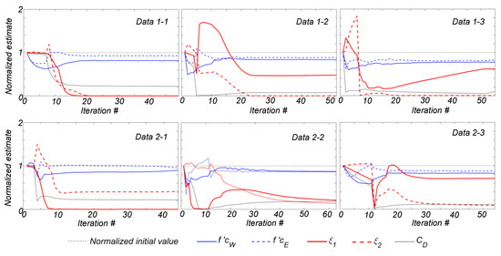
Figure 11.
Updating process for the posterior estimates of the unknown model parameters using data in Table 4.
Next, the prior estimates of responses—simulated responses using the prior FE model—and the posterior ones are compared with the field measurements. For the sake of brevity, only one second of data obtained using Data 1-2 are shown in Figure 12. In this figure, the two top rows correspond to channels 1–10 and an excitation frequency of 9.73 Hz, and the two bottom rows correspond to the same channels and an excitation frequency of 12.86 Hz. For the case of excitation frequency of 9.73 Hz, the prior FE responses mostly underestimate the measurements in channels located between the supports (channels 2, 3, 4, 7, 8, and 9) and slightly overestimate the responses in channels located on the overhang parts (channels 1, 5, 6, and 10). However, the responses in all channels are initially overestimated for the excitation frequency of 12.86 Hz. This shows that although the prior FE model matches the main modal signatures of the real structure, it cannot correctly predict the measurements in the time domain. As can be seen in Figure 12, after the application of Bayesian model updating, the updated FE model better fits the measurement responses in the time domain. This improvement is noticeable in various channels and for both excitation frequencies of 9.73 Hz and 12.86 Hz.
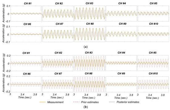
Figure 12.
The measured, prior and posterior estimates of FE-predicted responses using Bayesian FE model updating based on Data 1–2: (a) excitation frequency of 9.73 Hz and (b) excitation frequency of 12.86 Hz.
To quantify the discrepancies between two signals, the relative root mean square error (RRMSE) is calculated as follows:
In the above equation, and denotes the measured and estimated responses at the time step. The closer the RRMSE gets to zero, the better signals and match. The RRMSEs are calculated between the measured responses and their prior/posterior FE-predicted responses and are listed in Table 5.
Table 5.
RRMSEs (%) between the measurements and FE-predicted responses from the prior and posterior model.
As can be seen in Table 5, RRMSE values are reduced from prior to posterior values for all measurement channels. This shows that the time-domain model updating reduces the discrepancies between FE-predicted and measured responses successfully. However, the highest posterior RRMSEs are due to channels 1, 5, 6, and 10. These channels are located on the overhang parts of the girders (see Figure 4), and the measurements are likely less reliable due to the low signal-to-noise ratio. It is understandable from Figure 12 and Table 5 that the FE-predicted responses at these channels are promisingly updated to match the measurements.
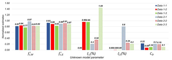
The final estimates of unknown model parameters using all data are shown in Figure 13. The average final estimates of parameters and are approximately 30% and 26% less than their initial values in Table 2. Previous studies [72,73] have shown more than 25% reductions in concrete compressive strength of deteriorated concrete structures—e.g., abandoned structures and structures in acidic environments. Considering that the operating environment of girders caused them to be prone to various damage mechanisms (including concrete degradation, as well as steel corrosion as discussed in Section 2.1.1), the final estimates of parameters and are reasonable. Moreover, as mentioned in Section 2.1.1, after being decommissioned, the west girder has been under more intense environmental testing conditions than the east girder [45]. This can be understood from the model updating results as the final estimates of parameter is smaller than . The only exception is the case study with Data 2-1 in which the final estimate of is smaller than . This is most probably an estimation error due to measurement noise, experimental error, etc. Moreover, based on Figure 13 and ignoring the case study with Data 2-1, the maximum difference in the estimation of parameter in layouts 1 and 2 is less than 7%, which shows the consistency of Bayesian model updating results regardless of the shaker location and target load amplitude.
The final estimates for modal damping parameters vary between different data sets. The identifiability analysis showed dependencies between parameters , , and . This dependency is most probably a reason for the discrepancy between the final estimates of these parameters using different data sets. Aside from this, it is known that structural damping roots in various factors, including opening and closing of micro cracks, friction in structural joints, level of vibration, and other sources of energy dissipation, etc. [74,75]. These conditions could be varied from one experiment to another and result in different levels of damping. To have insight into the overall damping of the testbed structure, the modal damping ratios are calculated using the state matrix of the system. For this purpose, the stiffness, mass, and damping matrices of the system are developed for the posterior models. The stiffness (K) matrix is recorded as the current global system matrix (using OpenSees printA command) while a static analysis using LoadControl integrator is carried out, and damping is removed from the model. The mass matrix (M) is calculated based on the current global system matrix while a static analysis using LoadControl integrator and a transient analysis using CentralDifference integrator is carried out, and damping is removed from the model. Using the Central Difference formulation presented in Equation (22), the mass matrix is equal to the recorded current global system matrix () times . In Equation (22), the term is the size of the time step increment and is set to a very small value (here s) to record the current global system matrix with high precision. The term C is the damping matrix.
Including damping in the model and carrying out a transient analysis using Newmark integrator with 0.5 and 0.25, the matrix can be recorded using printA. The damping matrix is calculated as it is shown in Equation (23) using the Newmark formulation.
The matrices M, C, and K are condensed at the dynamic DOFs, and the state matrix is calculated [74]. Using the state matrix of the posterior models, the modal damping ratios are obtained for all data sets. These damping ratios are reported in Figure 14. As can be seen, the testbed structure dissipates a greater level of energy in its first mode than in the second mode, which agrees with the identified modal damping ratios (see Table 1). Moreover, the overall modal damping ratios estimated from experiments with larger target load amplitudes are smaller than those estimated from experiments with smaller target load amplitudes. Although this has been previously observed in a few system identification studies [76,77], it is in contrast with the literature in which damping increases as load amplitude increases.
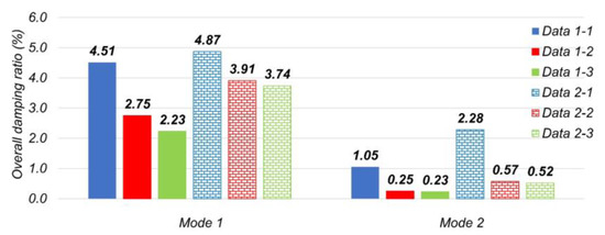
Figure 14.
Overall damping ratio of the testbed structure for mode 1 and mode 2 using different data sets.
4. Conclusions
This paper proposed a two-step FE model updating process for operational health monitoring and damage identification of bridge structures. In the proposed approach, first, modal-based model updating was carried out to calibrate the initial FE model of the bridge. In this step, the stiffness-related model parameters—mainly related to boundary conditions—as well as the initial stiffness of concrete material were updated to fit the FE-predicted and identified modal signatures of the bridge. Then, to account for the nonlinear response behavior of the bridge as well as refinement of model parameter estimation, Bayesian time-domain model updating was carried out in the second step. In this step, material properties that reflect the cumulative damage in the bridge, e.g., effective concrete compressive strength, as well as damping energy-dissipation-related model parameters, were estimated. The linear-elastic boundary conditions were fixed at their final estimates obtained from the modal-based model updating. To prevent convergence of the model updating algorithm to the local solution, the initial values for concrete compressive strength were selected using the final estimates of concrete initial stiffness from modal-based model updating.
The application of the two-step model updating approach was presented using a pair of full-scale precast prestressed deteriorated bridge I-girders as the testbed structure. For this study, a series of forced-vibration experiments were planned, and the testbed structure was subjected to sinusoidal force excitations through frequency sweeps at three different amplitudesusing a small shaker. The input excitation was measured using load cells, and the acceleration responses were collected using a wireless sensing network. The findings confirm the following conclusions:
- Identifiability analysis showed significant mutual dependency between different model parameters. This mutual dependency could lead to weak identifiability of model parameters in the traditional FE model updating process. The proposed two-step model updating helped with this challenge to update the most sensitive model parameters separately using modal-based and time-domain model updating.
- Sequential application of modal-based and time-domain model updating reduced the challenges due to ill-conditioning and modeling errors.
- It was demonstrated that the updated FE model using only modal-based model updating was not capable of reflecting true response behavior of the structure in time domain.
- Concrete compressive strength was correlated with damage/deterioration in the monitored structure and could be used to assess the health condition of the structure. In this study, a 30% reduction in concrete compressive strength from its nominal value correctly showed significant deterioration in the studied girders.
It is noteworthy to mention that although the input load in this study was different from the traffic load during the operation of bridges, it provided a real-world exercise to validate the capability of the two-step model updating approach for damage identification of bridge structures.
Author Contributions
Conceptualization, F.G., H.E. and E.T.; methodology, N.M., F.G., H.E. and E.T.; software, N.M. and F.G.; validation, N.M., F.G. and H.E.; formal analysis, N.M. and F.G.; investigation, N.M., F.G. and H.E.; resources, H.E., M.B. and E.T.; data curation, N.M., M.B. and E.A.; writing—original draft preparation, N.M.; writing—review and editing, N.M., F.G., H.E., M.B. and E.T.; visualization, N.M.; supervision, H.E. and E.T.; project administration, H.E. and M.B.; funding acquisition, H.E., M.B. and E.T. All authors have read and agreed to the published version of the manuscript.
Funding
This project was funded through the United States Department of Transportation Small Business Innovative Research (SBIR) program Phase II (Contract #6913G619C100048). The project resulted from the collaboration between S.C. Solutions, Inc., the leading small business, the University of California Los Angeles (UCLA), and the University of Nevada, Reno. Opinions and findings in this study are those of the authors and do not necessarily reflect the views of the sponsor.
Data Availability Statement
Data and materials supporting the results or analyses presented in this work are available upon reasonable request from the corresponding author.
Acknowledgments
Authors would like to acknowledge Hoda Azari (FHWA NDE Center) for making available the prestressed girder testbed at the Turner Fairbank Highway Research Center and Blake Cox (FHWA NDE Center), who aided during testing.
Conflicts of Interest
The authors declare no conflict of interest.
References
- Shahsavari, V.; Mehrkash, M.; Santini-Bell, E. Damage Detection and Decreased Load-Carrying Capacity Assessment of a Vertical-Lift Steel Truss Bridge. J. Perform. Constr. Facil. 2020, 34, 04019123. [Google Scholar] [CrossRef]
- ASCE. ASCE’s 2021 Infrastructure Report Card. 2021. Available online: https://infrastructurereportcard.org/cat-item/bridges/ (accessed on 1 May 2022).
- Friswell, M.; Mottershead, J. Finite Element Model Updating in Structural Dynamic; Springer: Berlin/Heidelberg, Germany, 1995. [Google Scholar] [CrossRef]
- Zapico, J.; González, M.; Friswell, M.; Taylor, C.; Crewe, A. Finite element model updating of a small scale bridge. J. Sound Vib. 2003, 268, 993–1012. [Google Scholar] [CrossRef]
- Xiao, X.; Xu, Y.; Zhu, Q. Multiscale modeling and model updating of a cable-stayed bridge. II: Model updating using modal frequencies and influence lines. J. Bridg. Eng. 2015, 20, 04014113. [Google Scholar] [CrossRef]
- Li, Y.; Astroza, R.; Conte, J.; Soto, P. Nonlinear FE model updating of seismic isolated bridge instrumented during the 2010 Mw 8.8 Maule-Chile Earthquake. Procedia Eng. 2017, 199, 3003–3008. [Google Scholar] [CrossRef]
- Taciroglu, E.; Shamsabadi, A.; Abazarsa, F.; Nigbor, R.; Ghahari, S. Comparative study of model predictions and data from the Caltrans-CSMIP bridge instrumentation program: A case study on the Eureka-Samoa channel bridge. Sacramento 2014. [Google Scholar] [CrossRef]
- Ereiz, S.; Duvnjak, I.; Jiménez-Alonso, J.F. Review of finite element model updating methods for structural applications. Structures 2022, 41, 684–723. [Google Scholar] [CrossRef]
- McCoy, R. HedegaardBrock, ShieldCarol, LindermanLauren, Updated long-term Bayesian Monitoring Strategy for time-dependent deflections of I-35W Saint Anthony Falls Bridge. In International Conference on Structural Health Monitoring of Intelligent Infrastructure: Transferring Research into Practice; SHMII: Porto, Portugal, 2021; pp. 1141–1147. Available online: https://experts.umn.edu/en/publications/updated-long-term-bayesian-monitoring-strategy-for-time-dependent (accessed on 1 November 2022).
- Teughels, A.; De Roeck, G. Structural damage identification of the highway bridge Z24 by FE model updating, J. Sound Vib. 2004, 278, 589–610. [Google Scholar] [CrossRef]
- Schlune, H.; PLoS, M.; Gylltoft, K. Improved bridge evaluation through finite element model updating using static and dynamic measurements. Eng. Struct. 2009, 31, 1477–1485. [Google Scholar] [CrossRef]
- Costa, C.; Arêde, A.; Costa, A.; Caetano, E.; Cunha, A.; Magalhaes, F. Updating numerical models of masonry arch bridges by operational modal analysis. Int. J. Archit. Herit. 2015, 9, 760–774. [Google Scholar] [CrossRef]
- He, L.; Reynders, E.; García-Palacios, J.; Marano, G.; Briseghella, B.; De Roeck, G. Wireless-based identification and model updating of a skewed highway bridge for structural health monitoring. Appl. Sci. 2020, 10, 2347. [Google Scholar] [CrossRef]
- Tran-Ngoc, H.; Khatir, S.; De Roeck, G.; Bui-Tien, T.; Nguyen-Ngoc, L.; Wahab, M.A. Model updating for nam O bridge using particle swarm optimization algorithm and genetic algorithm. Sensors 2018, 18, 4131. [Google Scholar] [CrossRef]
- Mottershead, J.; Friswell, M. Model updating in structural dynamics: A survey. J. Sound Vib. 1993, 167, 347–375. [Google Scholar] [CrossRef]
- Ghahari, F.; Malekghaini, N.; Ebrahimian, H.; Taciroglu, E. Bridge digital twinning using an output-only Bayesian model updating method and recorded seismic measurements. Sensors 2022, 22, 1278. [Google Scholar] [CrossRef] [PubMed]
- Abedin, M.; De Caso y Basalo, F.; Kiani, N.; Mehrabi, A.; Nanni, A. Bridge load testing and damage evaluation using model updating method. Eng. Struct. 2022, 252, 113648. [Google Scholar] [CrossRef]
- Magalhães, F.; Cunha, Á.; Caetano, E. Online automatic identification of the modal parameters of a long span arch bridge. Mech. Syst. Signal Process. 2009, 23, 316–329. [Google Scholar] [CrossRef]
- Juang, J.-N. Applied System Identification; Prentice Hall: Englewood Cliffs, NJ, USA, 1994. [Google Scholar]
- James, G., III; Carne, T.; Lauffer, J. The Natural Excitation Technique (NExT) for Modal Parameter Extraction from Operating Wind Turbines, United States. 1993. Available online: https://www.osti.gov/biblio/10139203 (accessed on 1 November 2021).
- Ljung, L. System Identification Theory for the User, 2nd ed.; Prentice Hall PTR: Upper Saddle River, NJ, USA, 1999. [Google Scholar]
- Ewins, D.J. Modal testing: Theory, Practice and Application, 2nd ed.; John Wiley & Sons: Hoboken, NJ, USA, 2009. [Google Scholar]
- Saidin, S.; Kudus, S.; Jamadin, A.; Anuar, M.; Amin, N.; Ibrahim, Z.; Zakaria, A.; Sugiura, K. Operational modal analysis and finite element model updating of ultra-high-performance concrete bridge based on ambient vibration test. Case Stud. Constr. Mater. 2022, 16, e01117. [Google Scholar] [CrossRef]
- Moaveni, B.; He, X.; Conte, J.; Restrepo, J. Damage identification study of a seven-story full-scale building slice tested on the UCSD-NEES shake table. Struct. Saf. 2010, 32, 347–356. [Google Scholar] [CrossRef]
- Farrar, C.; Baker, W.; Bell, T.; Cone, K.; Darling, T.; Duffey, T.; Eklund, A.; Migliori, A. Dynamic Characterization and Damage Detection in the I-40 Bridge Over the Rio Grande; LA-12767-M, Technical Report; U.S. Department of Energy: Los Alamos, NM, USA, 1994; pp. 1–153. [Google Scholar] [CrossRef]
- Farrar, C.; Cornwell, P. Structural Health Monitoring Studies of the Alamosa Canyon and I-40 Bridges; Technical Report; U.S. Department of Energy: Los Alamos, NM, USA, 2000. [Google Scholar] [CrossRef]
- Zheng, Y.; Wu, H.; You, X.; Xie, H. Model updating-based dynamic collapse analysis of a RC cable-stayed bridge under earthquakes. Structures 2022, 43, 1100–1113. [Google Scholar] [CrossRef]
- Ebrahimian, H.; Astroza, R.; Conte, J.; Papadimitriou, C. Bayesian optimal estimation for output-only nonlinear system and damage identification of civil structures. Struct. Control Heal. Monit. 2018, 25, e2128. [Google Scholar] [CrossRef]
- Zhou, X.; Kim, C.; Zhang, F.; Chang, K. Vibration-based Bayesian model updating of an actual steel truss bridge subjected to incremental damage. Eng. Struct. 2022, 260, 114226. [Google Scholar] [CrossRef]
- Xia, Z.; Li, A.; Li, J.; Shi, H.; Duan, M.; Zhou, G. Model updating of an existing bridge with high-dimensional variables using modified particle swarm optimization and ambient excitation data. Meas. J. Int. Meas. Confed. 2020, 159, 107754. [Google Scholar] [CrossRef]
- Fan, W.; Qiao, P. Vibration-based damage identification methods: A review and comparative study. Struct. Heal. Monit. 2011, 10, 83–111. [Google Scholar] [CrossRef]
- Saidin, S.; Kudus, S.; Jamadin, A.; Anuar, M.; Amin, N.; Ya, A.; Sugiura, K. Vibration-based approach for structural health monitoring of ultra-high-performance concrete bridge. Case Stud. Constr. Mater. 2023, 18, e01752. [Google Scholar] [CrossRef]
- Cheng, X.; Dong, J.; Cao, S.; Han, X.; Miao, C. Static and dynamic structural performances of a special-shaped concrete-filled steel tubular arch bridge in extreme events using a validated computational model. Arab. J. Sci. Eng. 2018, 43, 1839–1863. [Google Scholar] [CrossRef]
- Mao, J.; Wang, H.; Li, J. Bayesian finite element model updating of a long-span suspension bridge utilizing hybrid Monte Carlo simulation and Kriging predictor. KSCE J. Civ. Eng. 2020, 24, 569–579. [Google Scholar] [CrossRef]
- Dong, X.; Wang, Y. Finite element model. In Computing in Civil Engineering 2019: Smart Cities, Sustainability, and Resilienc; American Society of Civil Engineers: Reston, VA, USA, 2019; pp. 397–404. [Google Scholar]
- Fang, C.; Liu, H.; Lam, H.; Adeagbo, M.; Peng, H. Practical model updating of the Ting Kau bridge through the MCMC-based Bayesian algorithm utilizing measured modal parameters. Eng. Struct. 2022, 254, 113839. [Google Scholar] [CrossRef]
- Polanco, N.; May, G.; Hernandez, E. Finite element model updating of semi-composite bridge decks using operational acceleration measurements. Eng. Struct. 2016, 126, 264–277. [Google Scholar] [CrossRef]
- Shi, Z.; Hong, Y.; Yang, S. Updating boundary conditions for bridge structures using modal parameters. Eng. Struct. 2019, 196, 109346. [Google Scholar] [CrossRef]
- Chen, S.; Zhong, Q.; Hou, S.; Wu, G. Two-stage stochastic model updating method for highway bridges based on long-gauge strain sensing. Structures 2022, 37, 1165–1182. [Google Scholar] [CrossRef]
- Luo, L. Finite element model updating method for continuous girder bridges using monitoring responses and traffic videos. Struct. Control. Health Monit. 2022, 29, e3062. [Google Scholar] [CrossRef]
- Kim, S.; Kim, N.; Park, Y.; Jin, S. A sequential framework for improving identifiability of FE model updating using static and dynamic data. Sensors 2019, 19, 5099. [Google Scholar] [CrossRef]
- Azam, S.E.; Didyk, M.M.; Linzell, D.; Rageh, A. Experimental validation and numerical investigation of virtual strain sensing methods for steel railway bridges. J. Sound Vib. 2022, 537, 117207. [Google Scholar] [CrossRef]
- Ramancha, M.; Astroza, R.; Madarshahian, R.; Conte, J. Bayesian updating and identifiability assessment of nonlinear finite element models. Mech. Syst. Signal Process. 2022, 167, 108517. [Google Scholar] [CrossRef]
- Yu, E.; Taciroglu, E.; Wallace, J. Parameter identification of framed structures using an improved finite element model-updating method—Part I: Formulation and verification. Int. Assoc. Earthq. Eng. 2007, 36, 619–639. [Google Scholar] [CrossRef]
- Gucunski, N.; Lee, S.; Mazzotta, C.; Kee, S.; Pailes, B.; Fetrat, F. Protocols for Condition Assessment of Prestressed Concrete Girders using NDE and Physical Testing; Technical Report; Federal Highway Administrations: Washington, DC, USA, 2014. [Google Scholar]
- U.S. Department of Transportation, Federal Highway Administration. 2020. Available online: https://highways.dot.gov/research/turner-fairbank-highway-research-center/facility-overview (accessed on 1 November 2021).
- Adams, M.; Nicks, J.; Stabile, T. Thermal Activity of Geosynthetic Reinforced Soil Piers; IFCEE/ASCE: San Antonio, TX, USA, 2015. [Google Scholar] [CrossRef]
- Liu, P.C. Damage to concrete structures in a marine environment. Mater. Struct. 1997, 24, 302–307. [Google Scholar] [CrossRef]
- Parker Lord. 2022. Available online: https://www.microstrain.com (accessed on 1 August 2021).
- SensorConnect. 2022. Available online: https://www.microstrain.com/software/sensorconnect (accessed on 1 August 2021).
- Fulop, S.; Fitz, K. Algorithms for computing the time-corrected instantaneous frequency (reassigned) spectrogram, with applications. J. Acoust. Soc. Am. 2006, 119, 360–371. [Google Scholar] [CrossRef]
- Welch, P. The use of the fast fourier transform for the estimation of power spectra: A method based on time averaging over short, modified periodograms. IEEE Trans. Audio Electroacoust. 1967, 15, 70–73. [Google Scholar] [CrossRef]
- Overschee, P.; Moor, B. Subspace Identification for Linear Systems Theory—Implementation—Applications; Kluwer Academic Publishers: Dordrecht, The Netherlands, 1996. [Google Scholar] [CrossRef]
- Peeters, B.; De Roeck, G. Reference based stochastic subspace identification in Civil Engineering. Inverse Probl. Eng. 2000, 8, 47–74. [Google Scholar] [CrossRef]
- MathWorks, n4sid Estimate State-space Model. 2022. Available online: https://www.mathworks.com/help/ident/ref/n4sid.html (accessed on 1 April 2022).
- Bodeux, J.; Golinval, J. Application of ARMAV models to the identification and damage detection of mechanical and civil engineering structures. Smart Mater. Struct. 2001, 10, 479–489. [Google Scholar] [CrossRef]
- MathWorks, sset Estimate State-space Mode. 2022. Available online: https://www.mathworks.com/help/ident/ref/ssest.html (accessed on 1 April 2022).
- McKenna, F. OpenSees: A framework for earthquake engineering simulation. Comput. Sci. Eng. 2011, 13, 58–66. [Google Scholar] [CrossRef]
- Naeim, F.; Kelly, J. Design of Seismic Isolated Structures: From Theory to Practice; John Wiley & Sons: New York, NY, USA, 1999. [Google Scholar]
- Chopra, A. Dynamics of Structures, 4th, ed.; Prentice Hall: Upper Saddle River, NJ, USA, 1995. [Google Scholar]
- Nabiyan, M.; Khoshnoudian, F.; Moaveni, B.; Ebrahimian, H. Mechanics-based model updating for identification and virtual sensing of an offshore wind turbine using sparse measurements. Struct. Control Heal. Monit. 2021, 28. [Google Scholar] [CrossRef]
- MathWorks. Matlab R2022a. 2022. Available online: https://www.mathworks.com/?s_tid=gn_logo (accessed on 1 April 2022).
- MathWorks. fmincon Algorithms. 2022. Available online: https://www.mathworks.com/help/optim/ug/choosing-the-algorithm.html (accessed on 1 April 2022).
- Van Den Abeele, K. Damage assessment in reinforced concrete using nonlinear vibration techniques. AIP Conf. Proc. 2003, 30, 341–344. [Google Scholar] [CrossRef]
- Gucunski, N.; Imani, A.; Romero, F.; Nazarian, S.; Yuan, D.; Wiggenhauser, H.; Shokouhi, P.; Taffe, A.; Kutrubes, D. Nondestructive Testing to Identify Concrete Bridge Deck Deterioration; Transportation Research Board: Washington, DC, USA, 2013; Available online: https://nap.nationalacademies.org/catalog/22771/nondestructive-testing-to-identify-concrete-bridge-deck-deterioration (accessed on 1 November 2021).
- Fernandez, I.; Herrador, M.; Marí, A.; Bairán, J. Structural effects of steel reinforcement corrosion on statically indeterminate reinforced concrete members. Mater. Struct. Constr. 2016, 49, 4959–4973. [Google Scholar] [CrossRef]
- Zhu, W. Effect of Corrosion on The Mechanical Properties of the Corroded Reinforcement and the Residual Structural Performance of the Corroded Beams, Universite de Toulouse. 2015. Available online: https://tel.archives-ouvertes.fr/tel-01222175/document (accessed on 1 November 2021).
- Ebrahimian, H.; Astroza, R.; Conte, J.; Bitmead, R. Information-theoretic approach for identifiability assessment of nonlinear structural finite-element models. J. Eng. Mech. 2019, 145, 04019039. [Google Scholar] [CrossRef]
- Song, M.; Astroza, R.; Ebrahimian, H.; Moaveni, B.; Papadimitriou, C. Adaptive Kalman filters for nonlinear finite element model updating. Mech. Syst. Signal Process. 2020, 143, 106837. [Google Scholar] [CrossRef]
- Ebrahimian, H.; Kohler, M.; Massari, A.; Asimaki, D. Parametric estimation of dispersive viscoelastic layered media with application to structural health monitoring. Soil Dyn. Earthq. Eng. 2018, 105, 204–223. [Google Scholar] [CrossRef]
- Ebrahimian, H.; Astroza, R.; Conte, J. Extended Kalman filter for material parameter estimation in nonlinear structural finite element models using direct differentiation method. Earthq. Eng. Struct. Dyn. 2015, 44, 1495–1522. [Google Scholar] [CrossRef]
- Ismail, M.; Muhammad, B.; Ismail, M. Compressive strength loss and reinforcement degradations of reinforced concrete structure due to long-term exposure. Constr. Build. Mater. 2010, 24, 898–902. [Google Scholar] [CrossRef]
- Li, B.; Cai, L.; Wang, K.; Zhang, Y. Prediction of the residual strength for durability failure of concrete structure in acidic environments. J. Wuhan Univ. Technol. Mater. Sci. Ed. 2016, 31, 340–344. [Google Scholar] [CrossRef]
- Rainieri, C.; Fabbrocino, G.; Cosenza, E. Some remarks on experimental estimation of damping for seismic design of civil constructions. Shock Vib. 2010, 17, 383–395. [Google Scholar] [CrossRef]
- Liang, C.; Liu, T.; Xiao, J.; Zou, D.; Yang, Q. The damping property of recycled aggregate concrete. Constr. Build. Mater. 2016, 102, 834–842. [Google Scholar] [CrossRef]
- Chen, G.; Omenzetter, P.; Beskhyroun, S. Modal systems identification of an eleven-span concrete motorway off-ramp bridge using various excitations. Eng. Struct. 2021, 229, 111604. [Google Scholar] [CrossRef]
- Brownjohn, J.; Dumanoglu, A.; Severn, R.; Blakeborough, A. Ambient vibration survey of the bosporus suspension bridge. Int. Assoc. Earthq. Eng. 1989, 18, 263–283. [Google Scholar] [CrossRef]


Disclaimer/Publisher’s Note: The statements, opinions and data contained in all publications are solely those of the individual author(s) and contributor(s) and not of MDPI and/or the editor(s). MDPI and/or the editor(s) disclaim responsibility for any injury to people or property resulting from any ideas, methods, instructions or products referred to in the content. |
© 2023 by the authors. Licensee MDPI, Basel, Switzerland. This article is an open access article distributed under the terms and conditions of the Creative Commons Attribution (CC BY) license (https://creativecommons.org/licenses/by/4.0/).