Study of the Data Augmentation Approach for Building Energy Prediction beyond Historical Scenarios

Abstract

Building energy consumption predictive modeling using data-driven machine learning is currently highly prevalent. However, the model typically performs poorly when the predicted day’s energy consumption exceeds the upper bound of the historical data. In this study, energy consumption projections are examined outside of historical boundary scenarios, including three occupancy behavior data (HVAC system, lighting, and equipment) and three operating future scenarios (Scenario 1: utilization rate is highest simultaneously; Scenario 2: energy-saving lighting renovation; Scenario 3: the number of people working is decreased). We propose using data augmentation based on the occupancy behavior (DAOB) method, which expands the building’s three occupancy behaviors. The case study showed that, among the three future operating scenario prediction tasks, scenario 1’s performance was the least accurate, with an average relative error of 50.21% compared to the DAOB method’s average relative error of 7.07%. The average relative error in Scenario 2 decreased from 15.83% to 10.10%. The average relative error in Scenario 3 decreased from 20.97% to 6.5%. This provided an efficient method of combining physical models with data-driven models, which significantly increased robustness and reliability of the model.

1. Introduction

Modern intelligent technology has undergone rapid development and has been utilized in various industries to boost work efficiency. The application of intelligent technology in building operation management is trailing behind in comparison to the computer industry, and a trend has emerged of raising the level of building operation management [1]. Building energy consumption prediction (BECP) is a critical precaution for efficient building energy management, defect diagnostics, and demand-side management [2,3], which is especially useful for assessing operation strategies, start-stop control, energy efficiency, and economy of central air-conditioning systems in large buildings. As a result, accurate building energy prediction models are critical.

With the rapid growth of intelligent technology, researchers have implemented many data-based methods to deliver the BECP over the past 10 years [2]. Data-driven approaches are the most common method due to their high efficiency, accuracy, and ease. Initially, researchers employed traditional machine learning algorithms (e.g., artificial neural networks [4,5], support vector regression (SVR) [6], and random forest (RF) [7]. Extreme gradient boosting (XGB) [8] and stacking ensemble learning techniques [9,10] were later included. In addition, long short-term memory (LSTM) [11,12] and deep reinforcement learning (DRL) [13,14] are two deep learning algorithms [15] that have recently gained popularity. Fu et al. [16] proposed a deep-forest-based DQN (DF–DQN) method as an active exploration. Almost all machine learning techniques have been applied in the application of algorithms.

Algorithm-centric research broadens the feasibility of implementing new machine-learning techniques in the building energy sector. In the domain of building energy, data collection is more challenging compared to artificial intelligence applications such as voice recognition, and there are significant data discrepancies between various buildings. Nevertheless, it is difficult to create big data from a single building’s data. As a result, the building energy sector frequently has insufficient data, which makes it difficult to adopt algorithm-centric techniques. Researchers recently began to focus on data-centric methods and believe that data processing would result in stronger training effects of machine learning. To overcome the data imbalance, Zhang et al. [17] suggested a multi-model prediction approach based on clustering decision trees. By clustering decision trees to classify and divide operational data into six usable ratios, they improved the accuracy of machine learning-based predictions. Through cluster analysis, some researchers (e.g., Liu et al. [18], Chen et al. [19,20]) uncovered building energy consumption patterns and developed machine learning models for varied energy consumption patterns, which all had effective outcomes. In addition, Dong et al. [21] created an energy consumption pattern classification model based on a decision tree based on time-related criteria, separated energy consumption into four patterns, and then created an integrated learning algorithm for each pattern with positive results. Hong et al. [22] used the KNN algorithm to predict the hourly energy consumption of community buildings. Ten similar hourly energy consumption patterns for 2 years were clustered, and the predictions were accurate.

However, clustering and classification approaches are only applicable when the data are sufficient, but their efficiency is limited by small data samples. As a response, researchers began to investigate the possibility of data augmentation in the case of a limited training example [23,24]. Currently, there are two available techniques for data augmentation, which are employing similar building data and using a generative model to generate data. Gao et al. [25] claimed that the prediction accuracy of simple models could be greatly improved by using historical data from similar buildings when the reference value for a target building, with limited high-quality information available, must be improved. Li et al. [26] presented federated learning to handle the issue of exposing occupants’ privacy, and they found that the federated model achieved an average decrease of 25.4% in CV-root mean squared error (CV-RMSE). Ribeiro et al. [27] used merged data from similar buildings with varied distributions and seasonal profiles and showed that by integrating extra data from other schools, the proposed approach could improve energy forecasts for a school by 11.2%. Although the use of similar building data for transfer learning has brought relatively positive results, transfer results are limited by supporting operation management due to their different characteristics. In addition, some researchers have attempted to gather augmented data using a generative model. Tian et al. [28] found that fusing the data, created by the generative adversarial network with the initial limited amount of data, could produce better results than training on the original dataset. Fan et al. [29] augmented building operational data with conditional variational autoencoders and evaluated the model using actual energy data from 52 buildings. All the above-mentioned strategies applied data-driven methods to enrich the datasets and helped enhance the accuracy of energy consumption prediction even with limited historical data. The physical model method has always been essential and can be merged with data-driven methods [30] to develop hybrid model methods with little or no historical data. Sha et al. [31] created a vast amount of simulated data orthogonally based on key traits and trained a machine learning model based on the simulated data to estimate energy usage for new buildings without previous data. Qian et al. [32] merged physical simulation data with a tiny quantity of actual data to produce a training dataset and found that the prediction accuracy of building cooling and heating loads was improved. Lu et al. [33] generated data augmentation sources and adopted transfer learning-based data fusion methods with target-built calibrated simulation models. They found that the calibrated simulation models could provide high-quality supplemented data. Therefore, a hybrid method based on a data-driven approach and reinforced physical models may adapt to various predicted demand changes in a complete manner.

In summary, current studies have shown that data augmentation techniques can raise model stability. The current data augmentation techniques were developed using either mathematical techniques or physical model orthogonal experiments. While transfer learning and generative modeling techniques apply mathematical methodologies to the same architectural historical data, physical models are built using domain knowledge of building energy. Although many buildings have smart monitoring already installed and operational data being gathered, scenarios outside the realm of prior experience may still be possible. In this situation, data augmentation based on analogous structures and generative models is constrained and challenging to interpret. Physical model-based data augmentation can produce more accurate predictions and better explanations. Numerous studies have shown the significance of occupancy behavior data to building energy consumption [34,35,36]. However, the expansion of data augmentation studies to occupancy behavior-related schedules has received little attention from academics. A modeling approach based on data-driven algorithms will be used in the future to model energy consumption for the building operation stage, and many academics will adopt the approach of physical model-assisted modeling. This research further merges data-driven modeling and physical model simulation methodologies while considering the physical model data augmentation method of using occupancy behavior data to offer a fresh perspective on exploration.

In this research, based on a practical requirement for a project (with the object of a real green office building in Zhuhai, China), a comprehensive study was conducted to systematically explore using the occupancy behavior data from a building’s real operation to broaden future scenarios beyond historical boundaries. To tackle the issue of energy consumption prediction beyond the historical range, data augmentation based on the occupancy behavior (DAOB) method is suggested. To evaluate the DAOB method, this study considered three usage scenarios for three occupancies of the HVAC system, lighting, and equipment. Furthermore, three potential building consumption scenarios were devised using the scenario analysis method to evaluate the performance of the prediction model. In addition, the occupancy of the HVAC system was characterized by counting the utilization rate of the fan coil unit. The occupancy of lighting and equipment was calculated using energy consumption data in reverse. As a result, the primary innovation of this study was to create models based on these training samples to achieve higher predictive performance by considering the expansion of occupancy behavioral data. This paper is organized as follows. Section 2 presents the research outline, establishment, and calibration of physical models and data augmentation. Section 3 presents the case study of the building, including data used in detail and model implementation details. Section 4 analyzes the performances of the prediction models under three future scenarios. Section 5 discusses the results and conclusions are drawn in Section 6.

2. Methodology

2.1. Research Framework

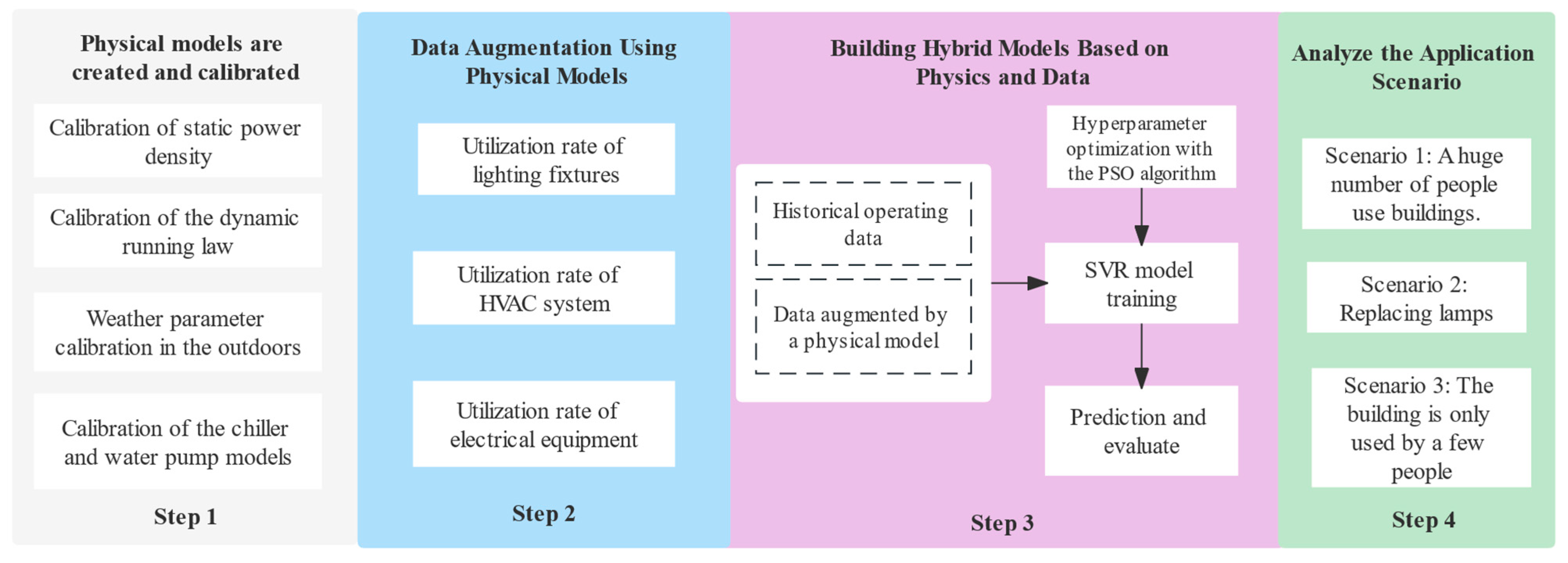
The schematic of this paper is shown in Figure 1. The data augmentation procedure was divided into four parts, which are described in detail as follows:

• Step 1. Creating and calibrating the physical models

A geometric model was created using building geometric structural information, and energy consumption was simulated using EnergyPlus software. The actual information was then calibrated depending on specific settings in the physical model so that the gap between the simulated and actual energy consumption levels could eventually be kept within an acceptable range.

• Step 2. Data augmentation

The building operating plan was adjusted based on the results of step 1. This stage covered the operating times for equipment, lighting, and HVAC. Scene presets were used to construct three ratios that corresponded to the real operation plan to depict potential future operating conditions. To combine 27 operation states and obtain the energy consumption simulation results for the corresponding operation states and the building operation states that could not be obtained in the historical operation, three conditions were set for the operation schedules for HVAC, lighting, and equipment.

• Step 3. Building the hybrid models

By combining the simulation data generated in Step 2 with historical experience, a hybrid model was created. The hyperparameters were set based on the particle swarm optimization (PSO) algorithm [37], and the machine learning algorithm adopted the conventional SVR algorithm.

• Step 4. Analyzing the scenario application

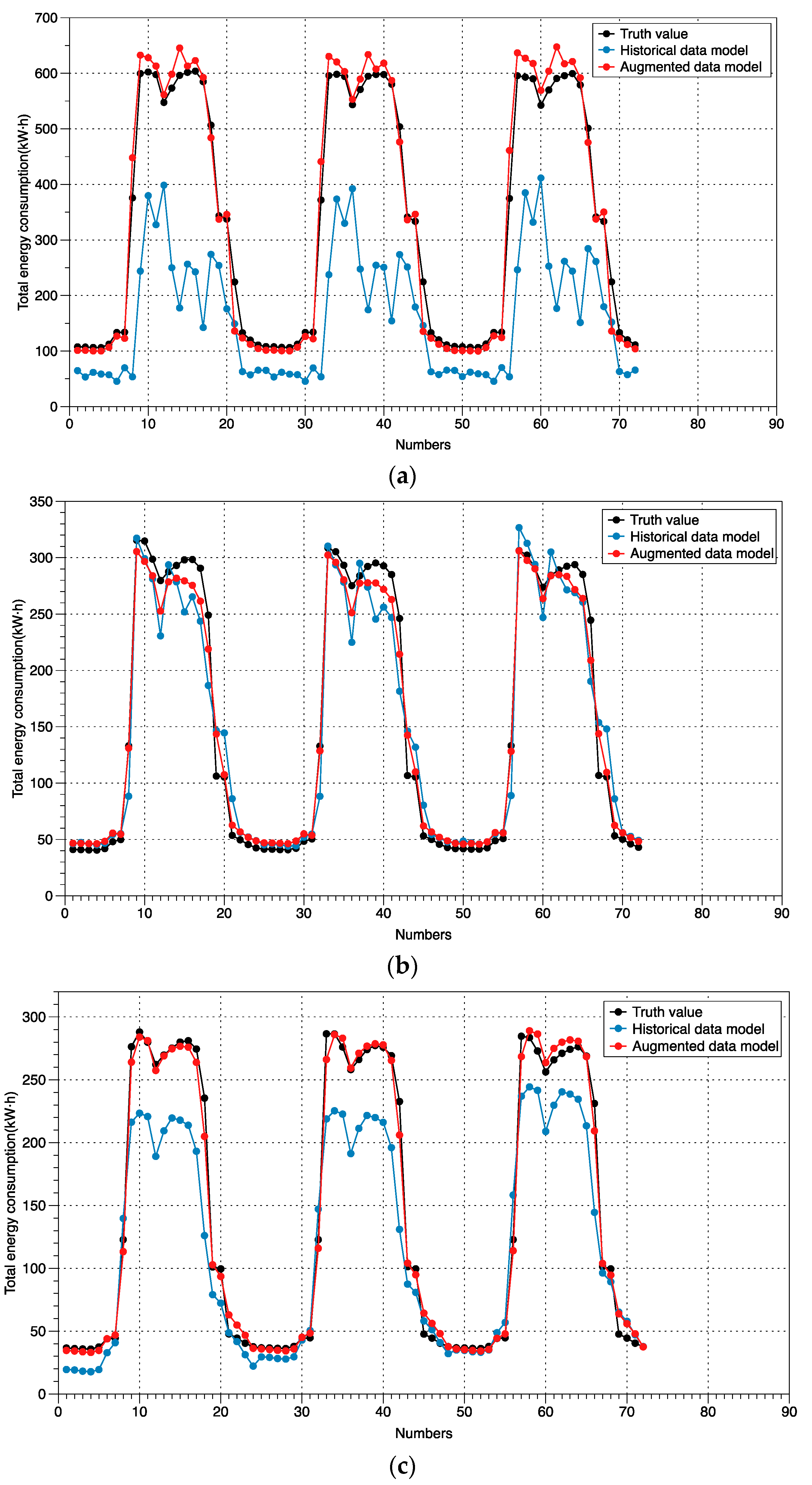
These three working scenarios outside historical experience were constructed to verify the effect of data augmentation. The assessment indicators showed the differences between the data augmentation modeling approach and the historical data modeling method.

2.2. Building and Calibrating Physical Models

Sketchup was used to create a physical building geometric model, and then EnergyPlus simulation software was used for energy consumption simulation. The energy consumption model was calibrated using accurate real-world building parameters, including static and dynamic parameters. The static parameters are adjusted based on the results of the survey. The schedules of the HVAC system and personnel were estimated according to the start and stop data of the fan coil units in the dynamic parameters. Lighting and equipment schedules were calculated by reversing the actual energy consumption. The outdoor weather was based on actual weather data.

Table 1. Calibration content of physical model input parameters.

Parameter Type	Parameters of Model	Default Settings	Actual Settings
static parameters	building envelope	architectural design parameters	actual implementation performance parameters
	personnel density	refer to China building energy efficiency design manual	refer to the as-built drawings and determine the number of seats according to the interior decoration
	lighting density		refer to the as-built drawings to count the power of lighting fixtures in each area
	equipment density		check with as-built drawings and equipment ledger
dynamic parameters	staff schedule	refer to similar buildings	calculate using the fan coil unit’s start-stop law
	lighting schedule		backward computation based on lighting energy usage data collected hourly
	equipment schedule		reverse computation using the device’s hourly energy consumption data
	HVAC system schedule		calculate using the fan coil unit’s start-stop law
	meteorological parameters	data for a typical meteorological year	real-time weather data for the building’s location over the period of a year
static/dynamic parameters	HVAC system parameters	reference design handbook	refer to the manufacturer’s sample data and as-built drawings

lists all of the calibration parameters for physical simulation.

2.3. Data Augmentation

The augmented dataset was obtained by altering the running schedule parameters in the calibrated physical model; thus, it could improve the prediction model’s inaccuracy caused by changes in the building operation.

Outdoor weather and internal occupancy behavior have a significant impact on a facility’s energy use in buildings. In this paper, only the parameter changes related to building occupancy behavior were considered. The parameters of the operating scene change included the HVAC, lighting, and electrical equipment operation schedules. Due to many possible combinations of the three factors, this study analyzed three levels of these three parameters compared to typical operating conditions, which were 0.3, 0.6, and 0.9, respectively. These numbers showed the utilization or proportion of equipment, lighting, and fan coils that were in use. A total of 27 operational scenarios were created by combining 3 operating levels and 3 schedules, and the 27 operating scenarios were then entered into the simulation software. In terms of technical implementation, finding the benchmark levels of 3 specific parameters was required for the combination of 27 sets of runtime data. The fan coil unit’s consumption level benchmark was a series of hourly averages of working days throughout a standard cooling season. The Fuzzy C-means (FCM) clustering approach was used to obtain a typical set of working days in the cooling season and then the mean value of the daily time series was used as the benchmark for lighting and electrical equipment utilization. Among them, the FCM clustering technique applied pattern recognition to establish a normal working pattern in the cooling season by analyzing 24-h lighting and electrical equipment energy consumption sequences in a year. Finally, proportional transformation was used to produce the three levels of each parameter and associated running schedule for each level.

When no other configuration settings changed, the 27 obtained groups of operating schedules were independently entered into the EnergyPlus(V8.0.1) software, which was created by the Lawrence Berkeley National Laboratory in California of the USA. To create an augmented dataset, the physical model was executed and the energy consumption for various operational conditions was calculated.

2.4. Data-Driven Modeling

2.4.1. SVR

Based on statistical learning theory, Vapnik [38] proposed the SVR classification algorithm in the mid-1990s. By developing the ε-insensitive loss function, Vapnik (1999) expanded it to SVR, which was utilized to address nonlinear regression issues. The SVR model was based on structural risk minimization. The model’s prediction ability for new samples (model generalization ability) was improved and the structural risk function was introduced to alleviate the problem of overfitting. The goal of structural risk minimization was to create a compromise between empirical risk and the Vapnik-Chervonenkis dimension, resulting in an improved model with high prediction accuracy and good generalization ability.

2.4.2. Hyperparameter Optimization

PSO was used to optimize the hyperparameters in the SVR modeling process in this research. In parameter optimization research, this strategy is commonly employed as the PSO algorithm has a faster convergence time and requires fewer parameters to set than other optimization techniques.

2.4.3. Performance Evaluation Indices

To assess the model’s performance, a performance evaluation index was required. The following were the evaluation indicators:

Mean relative error (MRE):

$$MRE=\frac{1}{m}{\displaystyle \sum }_{i=1}^m\left|\frac{E^{\left(i\right)}-{\widehat{E}}^{\left(i\right)}}{{\widehat{E}}^{\left(i\right)}}\right|$$

(1)

Mean absolute error (MAE):

$$MAE=\frac{1}{m}{\displaystyle \sum }_{i=1}^m\left|E^{\left(i\right)}-{\widehat{E}}^{\left(i\right)}\right|$$

(2)

Root mean square error (RMSE):

$$RMSE=\sqrt{\frac{1}{m}{\displaystyle \sum }_{i=1}^m{\left(E^{\left(i\right)}-{\widehat{E}}^{\left(i\right)}\right)}^2}$$

(3)

R-square(R²):

$$R^2=1-\frac{{{\displaystyle \sum }}_{i=1}^m{\left(E^{\left(i\right)}-{\widehat{E}}^{\left(i\right)}\right)}^2}{{{\displaystyle \sum }}_{i=1}^m{\left(E^{\left(i\right)}-\overline{E}\right)}^2}$$

(4)

where $m$ is the number of samples, $E^{\left(i\right)}$ is the true power consumption density of the sample at time $i$,$\mathrm{W}/{\mathrm{m}}^2$. ${\widehat{E}}^{\left(i\right)}$ is the predicted power consumption density of the sample at time $i$, $\mathrm{W}/{\mathrm{m}}^2$. $\overline{E}$ is the true average of power consumption density,$\mathrm{W}/{\mathrm{m}}^2$.

For the methods listed above, SketchUp was used to create the architectural geometric model, while EnergyPlus software was used to complete the energy consumption simulation. The SVR algorithm was used with the Scikit-learn(V0.21) software and the data-driven method was built in Python 3.7.

3. Case Study

The predicted demand for energy consumption served as the basis for this study. This study’s attention was on the South China commercial headquarters’ office building’ therefore, the test data were obtained from this particular case.

3.1. Building Description

The building contains 17 levels with an equipment room on the first floor and a product display space and a recreational reception area on the ground floor; the other floors serve as general office space, 13 of which are multi-functional floors. The structure is an example of ultra-low-energy green construction.

The building has a fairly comprehensive building energy consumption monitoring platform that can obtain hourly energy consumption data (e.g., lighting electricity, socket electricity, air conditioning electricity, power consumption, special electricity consumption) and data for corresponding functional areas, such as energy consumption data for the equipment’s sub-items, of which the particular electricity consumption is primarily the electricity consumption of the building’s information room. Furthermore, sensors collect data on interior and exterior environmental factors (e.g., indoor temperature, indoor relative humidity, outdoor temperature, outdoor relative humidity, outdoor wind speed) and monitor the building use conditions.

The necessary operational data for the entire year of 2018 and building geometric parameters (e.g., building shape, design drawings, and other data) were obtained. From 15 May to 24 August 2018, the actual operational data were selected, which included total energy, air conditioning energy, lighting energy, and socket energy consumption and 482 fan coil start and stop data. Furthermore, the dry bulb temperature data were included in the outdoor meteorological data.

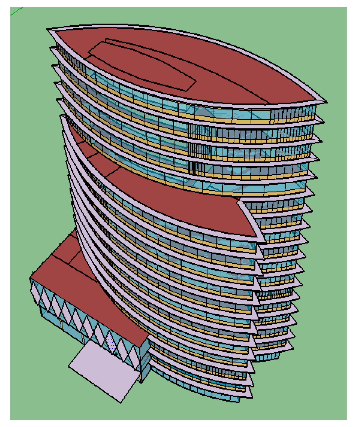
As shown in Figure 2, a physical geometric model was created based on the detailed building geometry and associated factors. The geometric model was then imported into EnergyPlus, where the required parameters were calibrated. The model generated energy consumption data that were physically simulated. Finally, to acquire valid physical simulation data, the simulation findings of the physical model were validated by comparing simulation data with actual operating data.

Table 2. Physical model parameters for thermal properties.

Items		Case
size (m2)		23,471
height (m)		73
shading coefficient		0.35
window-wall ratio	east	0.45
	south
	west
	north
U-value (W/(m2·K))	roof	0.40
	external wall	0.44
	external window	2.362

shows the physical model’s thermal profile parameter settings.

3.2. Calibration for Physical Models

Before being regarded as being close to the actual building, the model created based on the geometric shape of the building must be calibrated using real data. Both static and dynamic parameters will be used to calibrate the physical model’s parameter settings.

3.2.1. Static Power Density Parameters

In comparison to the design stage, the static power density parameter will alter during the building operation phase. Additionally, there are significant differences in the building’s specific operation mode, personnel behavior, and management mode. The lighting and equipment power densities were calculated statistically using the project’s as-built drawings and equipment ledger. The power density of a chiller was defined as the ratio of the chiller’s rated power to the total area of the building. The number of stations in the building operating stage was used to calculate the staff density.

The default settings of power densities were all larger than the actual ones, which was substantially lower than the default setting because the office building employs Light Emitting Diode (LED) lights and the values in the design manual refer to incandescent lamps, as indicated in

Table 3. Calibration comparison of static power density parameters.

—	Lighting (W/m2)	Equipment (W/m2)	Chiller (W/m2)	Area per Capita (m2/per)
default settings	10.28	15.35	21.81	5.58
actual settings	2.53	9.63	13.89	28.48

.

3.2.2. Dynamic Parameters

• Runtime schedule parameters

The dynamic operating characteristics of different buildings vary substantially, which is mainly caused by the varied structures’ operation methods, occupant patterns, and management modes. The associated operating schedule is created based on the energy consumption of each monitored sub-item and the operational status monitoring data.

The HVAC system’s ultimate operation schedule is for the building’s automatic control system to monitor the fan coil’s start and stop rules. The fan coil unit utilization rate was the chiller’s operating schedule. The office staff’s schedule in the room was determined by the fraction of fan coil units that were in operation during the summer. Simultaneously, from 10:00 p.m. to 7:00 a.m. the next day, the number of personnel working in the facility was planned to be unmanned. The variation in the fan coil unit’s utilization rate is depicted in Figure 3a. The proportion of use on working days was low compared to the default setting, while the proportion of use on non-working days was high. By dividing the current usage by the entire quantity, the utilization rate computation in Figure 3 was produced. For instance, the number of fan coils currently in operation divided by the total number of fan coils in the building gave the hourly utilization rate of fan coils. By dividing the hourly energy consumption by the total power of the lighting and equipment in the building, the hourly utilization rate of lighting and equipment could be calculated.

The ratio of the monitored hourly energy consumption data to the matching installed power was, namely, the operating schedule of lights and electrical equipment. Actual operating settings vs. default settings for typical day types are presented in Figure 3b,c. The actual lighting and electrical equipment operating schedules were lower than the default setting during working hours but higher than the default setting during rest time. Furthermore, the actual running time varied from day to day due to lunch breaks and overtime at night.

2.

Meteorological Parameters

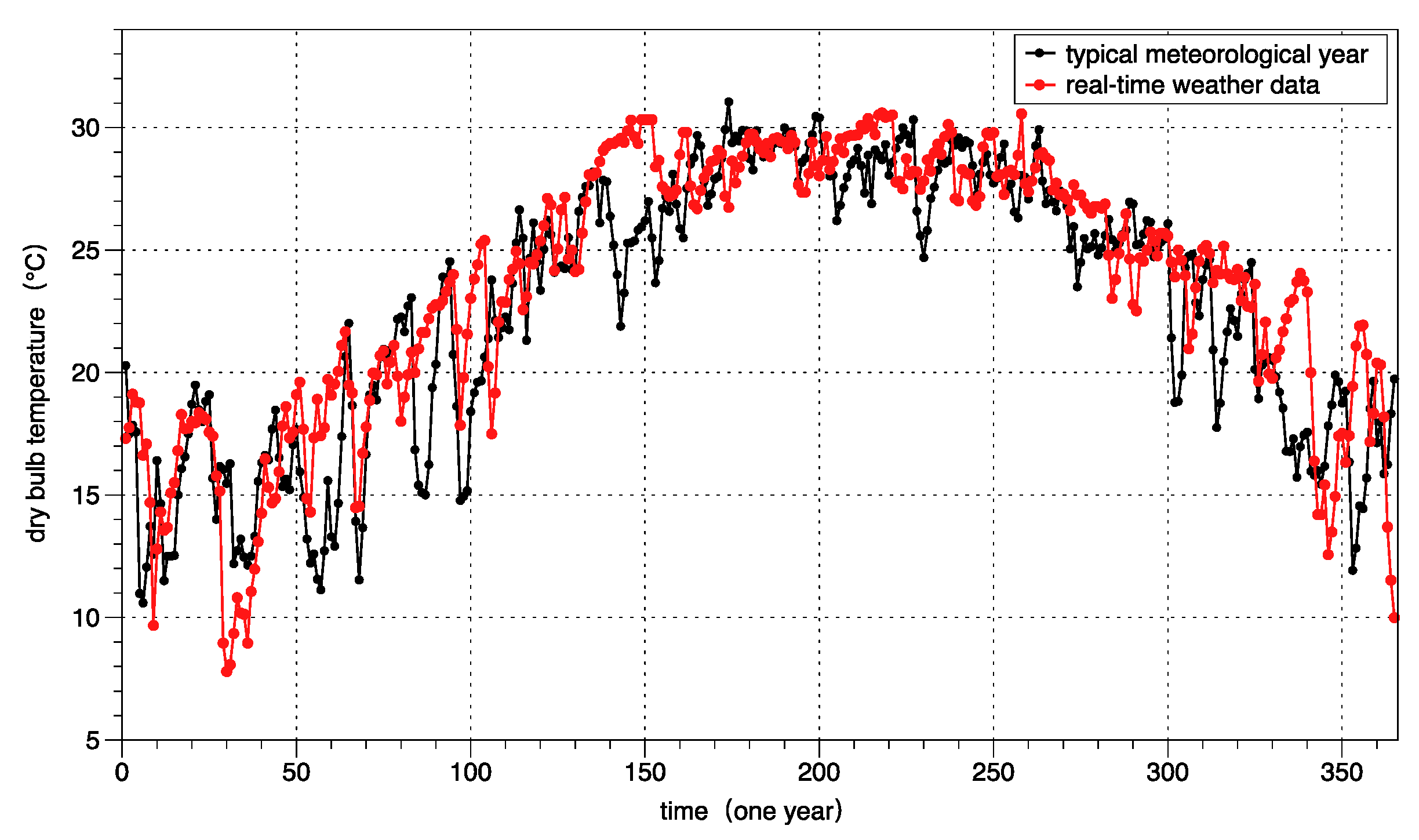
The effects of outdoor meteorological conditions on building load and energy consumption are significant; thus, outdoor meteorological conditions are used in most physical model simulations. Typical meteorological annual data are based on the statistical processing of meteorological observation data in the region over 10 years with statistical significance. However, because the energy consumption model used to guide a given optimization process must make predictions based on real-time meteorological parameters or forecast data, the meteorological parameter values must be calibrated.

The outdoor meteorological input parameters for calibration were received from the local meteorological station and utilized as the annual hourly meteorological data for the subsequent year (2018).

Table 4. Meteorological comparison of actual meteorological year and typical meteorological year.

—	Dry Bulb Temperature (°C)	Dew Point Temperature (℃)	Relative Humidity	Wind Speed (m/s)
typical meteorological year	22.71	19.25	81.67%	3.26
real-time weather data	23.57	20.00	80.80%	4.90
rate of deviation	3.76%	3.91%	−1.06%	50.47%

shows the actual meteorological data and typical meteorological annual data (e.g., the actual outdoor dry bulb temperature, dew point temperature, relative humidity, and wind speed). Aside from relative humidity, which was slightly lower, the rest data were all higher than the typical meteorological annual data. The annual daily average temperature changes of the actual meteorological annual data and usual meteorological annual data are shown in Figure 4.

3.

HVAC System Parameters

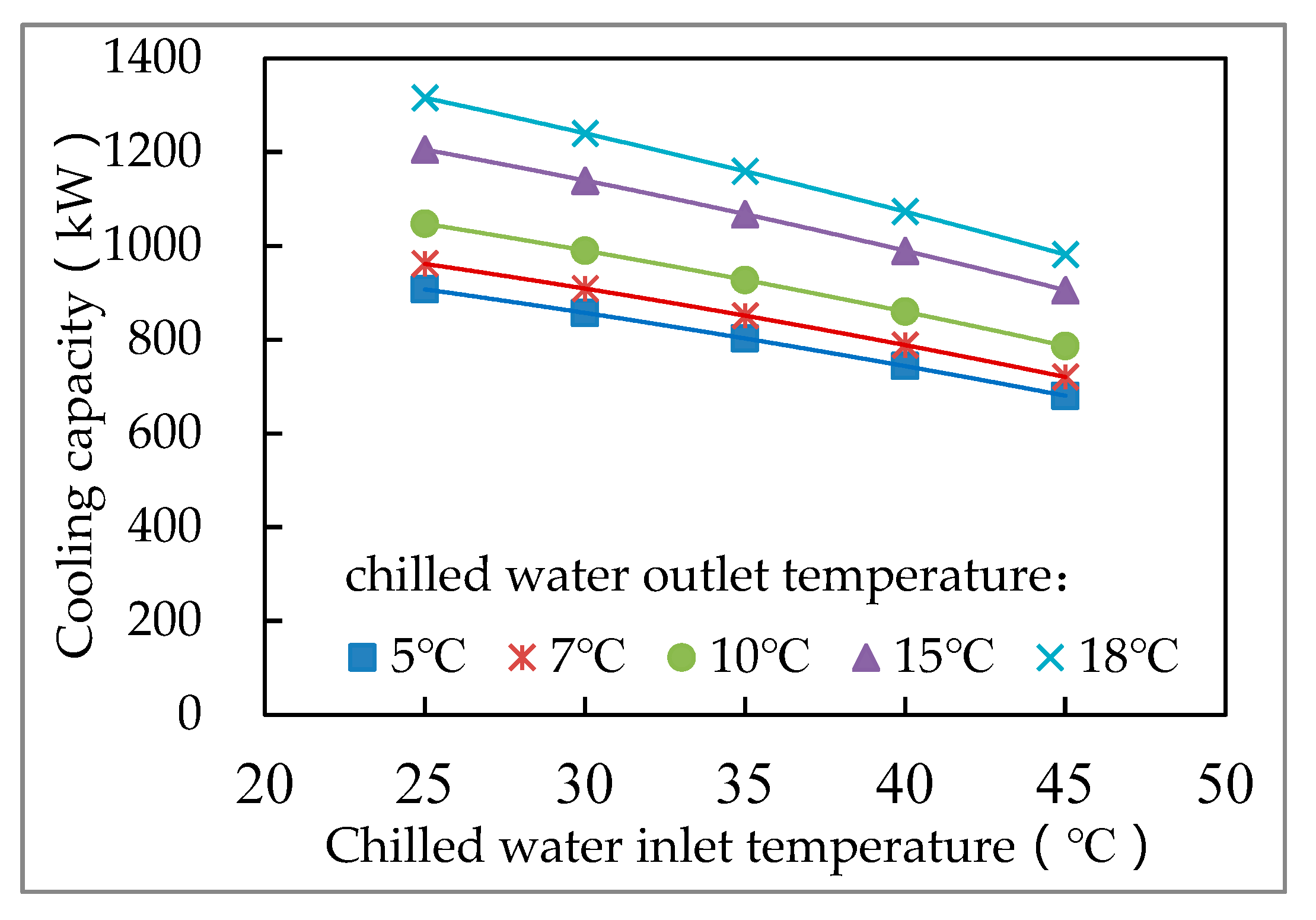
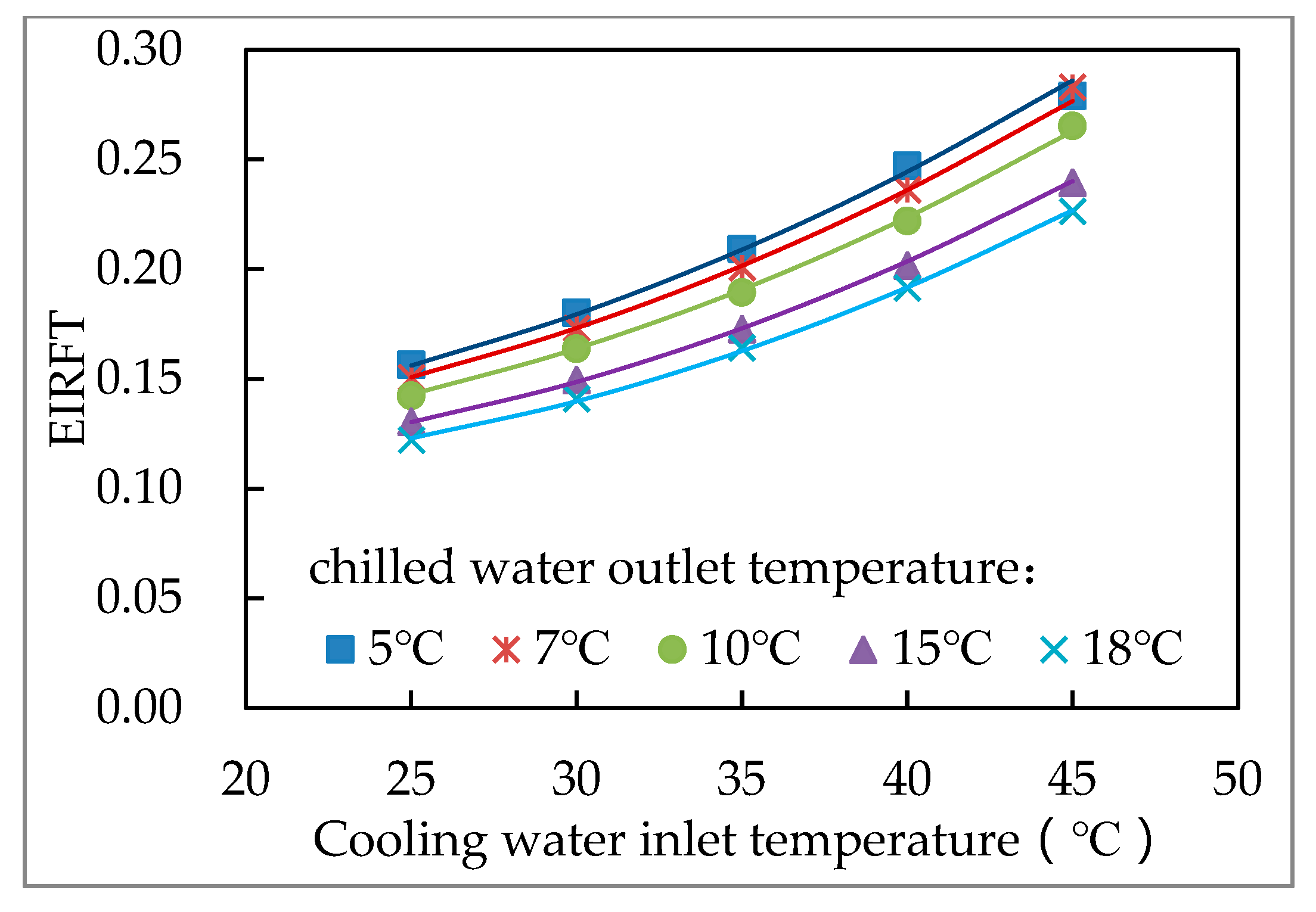
Choosing the right chiller and water pump models is critical for improving energy simulation accuracy. The chiller model in EnergyPlus was adapted from DOE-2, which is composed of three equations. The fitting was conducted according to the chiller manufacturer’s reference data and the effective unit operation data were obtained by processing the HVAC system’s operation data, which included the temperature of the cooling water inlet and outlet, the chiller’s cooling capacity, and the energy consumption of the cooling water and chilled water pumps. Finally, the following HVAC models were obtained. Additionally, fan coil units were used at the system’s termination, and the wind speed was controlled automatically.

• Chiller model:

Based on the manufacturer-provided reference data for the HVAC system equipment, performance curve fitting was conducted in this study. As shown in Figure 5, the chilled water output temperature and cooling water inlet temperature had an impact on the chiller’s cooling capability. As demonstrated in Figure 6, the chilled water outlet temperature and cooling water inlet temperature had an impact on the chiller’s ability to cool. The chiller’s capacity to cool Figure 7 depicts the impact of partial load rate.

$$\begin{gathered} CAPFT=0.97950+0.03735\times T_{chws}+0.00036\times T_{chws}^2 \\ -0.00206\times T_{con}-0.00012\times T_{con}^2-0.00044\times T_{chws}\times T_{con} \end{gathered}$$

(5)

$$\begin{gathered} EIRFT=0.75776-0.00161\times T_{chws}+0.00006\times T_{chws}^2 \\ -0.00857\times T_{con}+0.00070\times T_{con}^2-0.00058\times T_{chws}\times T_{con} \end{gathered}$$

(6)

$$EIRFPLR=0.54883-0.49671\times CPLR+0.95895\times CPL{R}^2$$

(7)

Among them, $CAPFT$ is the change of the cooling capacity of the chiller with the temperatures of the chilled and cooling water. $EIRFT$ is the variation of chiller cooling efficiency with chilled and cooling water temperature. EIRFPLR is the change in the cooling efficiency of the chiller with the partial load rate. $T_{chws}$ is the chilled water outlet temperature ℃., $T_{con}$ is the cooling water inlet temperature, ℃. and $CPLR$ is the partial load rate of the chiller.

• Pump model:

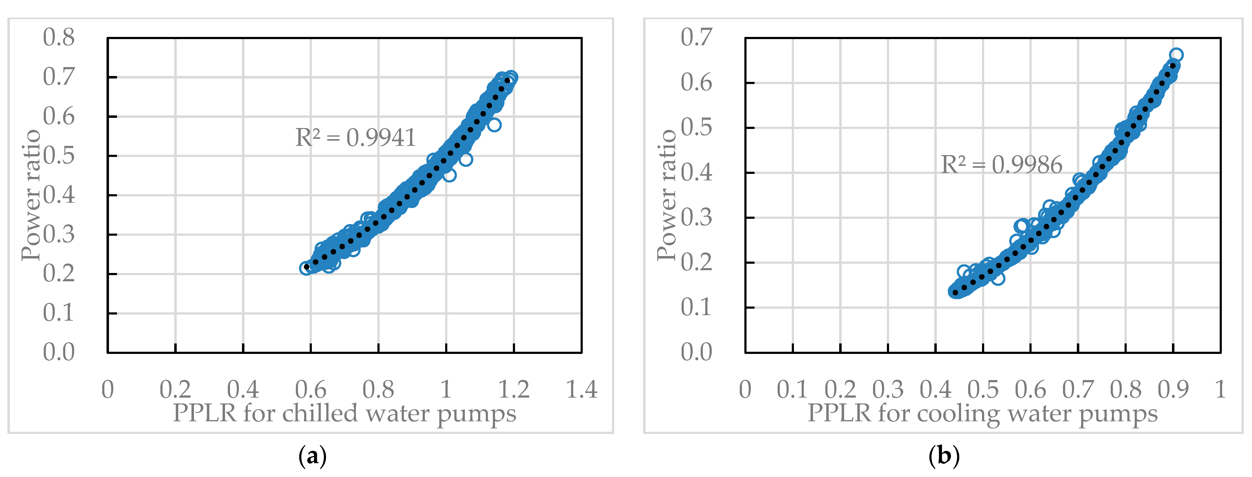
The usual fixed-frequency and variable-frequency water pumps were both represented in the EnergyPlus software’s water pump model. According to real-world circumstances, this study used variable-frequency water pumps for chilled and cooling water pumps. After data preprocessing, 1633 sets of chilled water pumps and 1967 sets of effective data for cooling water pumps were retrieved from the operating data of the air conditioning system on the management platform, respectively. Polynomial fitting was then carried out, as shown in Figure 8a,b.

Chilled water pump:

$$FrFLP=0.0596+0.1881\times PLR-0.0136\times PPL{R}^2+0.2610\times PPL{R}^3$$

(8)

Cooling water pump:

$$FrFLP=0.0069+0.1148\times PPLR-0.1375\times PPL{R}^2+0.5732\times PPL{R}^3$$

(9)

where $FrFLP$ is the ratio of pump input power to rated power. P$PLR$ is the ratio of the pump delivery flow to the rated flow.

3.3. Data Augmentation

According to the baseline in Figure 9a–c, the actual operation schedule (utilization rate) fluctuated between 25% and 45%, with lighting being low and the electrical equipment and HVAC system being closed. The enhanced operating schedule of the three parameters (lighting, electrical equipment, and fan coil from a minimum of 0.3 to a maximum of 0.9) was obtained using the enhancement approach, as shown in Figure 9a–c. The 27 combinations obtained were sent into the physical model, which produced hourly simulated energy use as augmented data.

4. Results

Based on the calibration of the physical model as outlined in Section 3.2, data augmentation was carried out. As a result, this section presents the data expansion verification and physical model calibration in three different scenarios.

4.1. Performance of the Calibration

As shown in Figure 10, the black points in the picture reflect the calibrated physical model’s simulated monthly energy intensity (a building’s total energy consumption divided by its total building area in a month), whereas the red points in the figure represent the case building’s real monthly energy intensity. The graphic illustrates how well the simulation results after calibration match the data on energy consumption. By dividing the difference between the actual energy consumption and the simulated energy consumption by the actual energy consumption, the monthly error rate can be calculated. The error rate of monthly energy consumption was within 5%, as illustrated in Figure 11, where the black histogram depicts the error rate for each month and the red straight line represents the 5% error line. Furthermore, it satisfied the ASHRAE Guideline 14 [39] accuracy requirements. As a result, the calibrated physical model is trustworthy and can be employed for data augmentation assistance.

4.2. Performance of Data Augmentation

This study specified three typical situations with major changes in routines for verification to check the performance of data augmentation, and the scenarios did not arise in the historical range.

The three scenarios were created as follows:

• Scenario 1: Each item’s utilization rate was highest simultaneously.

Each item’s utilization rate is the highest, with lighting, electrical equipment, and the fan coil unit all reaching 100% utilization simultaneously, assuming that the operation maintained the previous pattern on 20 and 21 August but that the intensity of building usage increased dramatically on 22 August and onwards. This is the first time in history that the usage rate of lighting, electrical equipment, and air-conditioning terminals all reached 100%. Figure 12a depicts its operating schedule.

• Scenario 2: Energy-saving lighting renovation.

The building is upgraded for energy efficiency and more efficient lighting fixtures are installed. Assuming that the lighting remains unchanged on 20 and 21 August and that all lamps are replaced with more efficient energy-saving lamps from 22 August, the lighting utilization rate is equivalent to a 50% reduction, while the electrical equipment and fan coil unit utilization rates remain unchanged; the operating schedule at this time is shown in Figure 12b.

• Scenario 3: The number of people working in the office is decreased.

Due to the present epidemic, office personnel density has decreased, and fewer office personnel and office equipment are housed in the same building area. The restart rate is only 73% and the utilization rate of the fan coil units is lowered to 92% of the baseline, assuming that the density of office workers remains unchanged on 20 and 21 August, and due to the impact of the epidemic on 22 August and thereafter. For appliances powered by electricity, the equipment utilization rate is 81% of the baseline, while the lighting fixture utilization rate is 92% of the baseline. Figure 12c depicts the operating schedule during this period.

According to the data-driven modeling method, the augmented and historical datasets were modeled independently. Figure 13 shows the model effect verification of the preceding three hypothetical scenarios, while

Table 5. Prediction error comparison under three application scenarios.

Evaluation Index	Scenario 1		Scenario 2		Scenario 3
	Historical Data Model	Augmented Data Model	Historical Data Model	Augmented Data Model	Historical Data Model	Augmented Data Model
MRE	50.21%	7.07%	15.83%	10.10%	20.97%	6.50%
MAE	178.63	20.74	19.74	11.07	31.03	5.97
RMSE	223.31	30.10	26.57	14.64	41.57	8.70
R2	0.70	0.98	0.954	0.99	0.95	0.99

shows the statistical model flaws based on historical and augmented data. The prediction accuracy of the data-driven model based on the historical dataset was dramatically lowered for scenario 1, and its average relative error reached 50.21%, indicating its failure in abrupt occurrences. With an average relative error of 7.07%, the data-augmented hybrid model could make more precise predictions. In scenario 2, the average relative errors predicted by the two types of model techniques were 15.83% and 10.10%, respectively, whereas the average relative errors were 20.97% and 6.50%, respectively in scenario 3. The data augmentation strategy presented in this research could successfully improve the resilience of the prediction model beyond historical experience, as demonstrated by the verification of the three scenarios.

5. Discussion

Based on the proposed DAOB method, this section discusses its adaptability, limitations, and research potential regarding the framework, calibration, and data augmentation. In the task of building energy consumption prediction, machine learning model approaches alone have shown limitations [40]. Additionally, the hybrid method, which integrates physical model data and historical data methods, has a certain flexibility and has received extensive attention from scholars. We would like to highlight that data-driven methods based on historical data perform well in coping with energy consumption predictions within the range of historical experience. However, its performance is poor in the face of predictions beyond the range of historical experience. Therefore, it is essential to research ways to circumvent the training dataset’s constraints during the data-driven modeling process. How to include domain information in the modeling process has been extensively researched [41,42]. Mohammadiziazi et al. [43] emphasized the value of gathering data on the occupant, operation, HVAC system, and weather-related parameters. Without considering the unpredictability of occupancy behavior, Zhu et al. [44] inserted three common scenarios for the running schedule while creating the fundamental dataset through the physical model to explore the variable set problem. Kim et al. [45] noted that occupancy behavior strongly influences the model’s performance, and the occupant data for each zone were created using the LBNL occupancy simulator at 5-min intervals without using actual occupancy behavior data. The DAOB method suggested in this study uses data-driven modeling as the primary approach and a physical model as an auxiliary approach. It also factors in the influence of occupancy behavior, which further enhances the predictability of the model. This method has been verified in this paper. Future research on this technique framework must be conducted in greater detail.

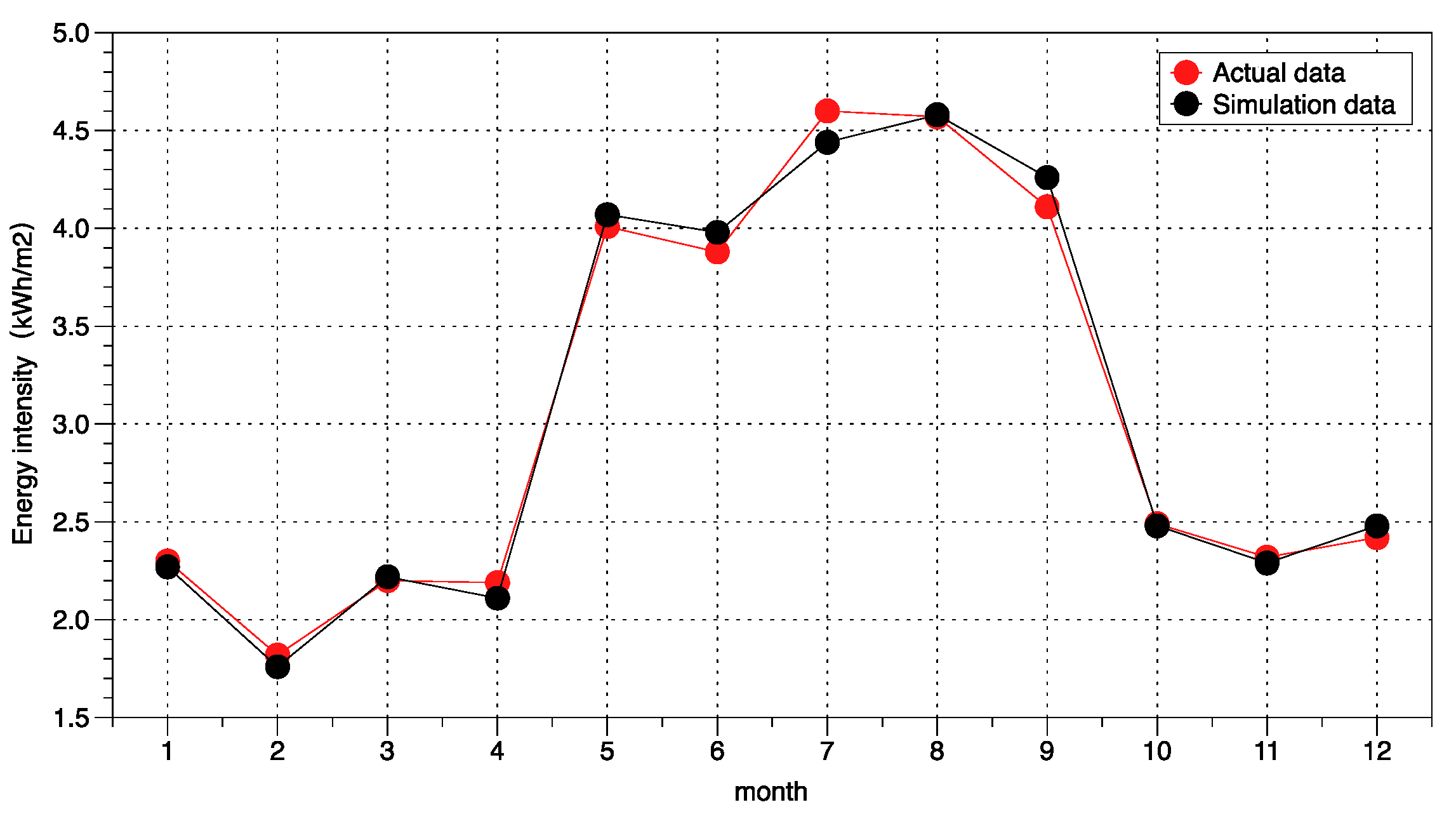
For the physical model calibration in this paper, we used the monthly standard error as the evaluation. Here, detailed information has been characterized, especially since the opening rate of the actual fan coil was used to characterize the work and rest schedules of the HVAC system. After detailed calibration of actual information, the energy consumption results of the physical model were close enough to the actual situation and possibly allowed for subsequent data enhancement. Of course, follow-up research can be carried out to further improve the reliability of the physical model with detailed time-to-calibration data. The model calibration portion of this study used the manual calibration method rather than automatic calibration because it focused on data augmentation research. In the future, auto-calibration will be preferable [46].

The SVR algorithm was employed in the machine learning algorithm in this study. Its benefit stems from the kernel function’s inclusion, which enables nonlinear mapping in a high-dimensional space. Additionally, structural risk minimization enhances the model’s capacity for generalization. Last but not least, the SVR algorithm has a strong theoretical basis in the form of the duality theory and the same continuation theory. Of course, the SVR method has limitations for large datasets, despite certain advantages in short samples. The SVR algorithm should be employed with care when working with large amounts of data. Additionally, SVR is sensitive to anomalous data; thus, it is important to ensure that the data are accurate before employing it.

According to the assumption of this paper, the data enhancement adopted three levels of running schedules, and more enhancement methods can be further considered in the future. In addition, three future scenarios beyond historical experience were designed according to the usage of buildings as verification, and the fusion verification of two types of datasets was considered. We find that building hybrid models with datasets augmented by physical models is more beneficial as the operating scenarios were enriched by physical models. Of course, after the building has accumulated more than 1 year of operational data, the use of data augmentation for physical models is relatively reduced. Therefore, the DAOB method suggested in this research is an auxiliary method that only generates a positive effect when combined with data-driven integration based on historical data. Paying attention to the application boundaries during the application process is important.

6. Conclusions

This study investigated an occupancy behavior-based data augmentation technique for building energy prediction. Operating schedules for HVAC, lighting, and equipment relevant to occupant behavior were added to a physical model that had been calibrated as the foundation. Finally, three potential future building operating scenarios were used to assess the efficacy of the technique, and the prediction findings from the extended dataset were contrasted with those based solely on historical data. The study showed that in predicting jobs outside the scope of historical scenarios, data augmentation taking occupancy behavior into account based on a calibrated physical model resulted in a more stable and accurate prediction model. The building’s basic utilization rates for equipment, lighting, and air conditioning were found to be approximately 0.4, 0.2, and 0.4, respectively, after an analysis of how the building operates. This means that it was difficult for operational behavior below or above these levels to appear in the actual operational data. As a result, the three settings outside of the operating scenarios that were recognized in this study broaden the application of data and enhance the adaptability of data-driven models.

The method described in this paper helps improve the interpretation of the data-driven model and provides a method for the fusion of the physical and data-driven models, which is necessary for the building operation phase to improve the adaptability of the energy consumption prediction model. This could support the development of stable energy consumption prediction models for future energy management systems, particularly in the event of sudden, sporadic projections that go beyond historical data. The physical model was employed as a tool for data expansion, but the fundamental model adopted was still data-driven. The proposed DAOB method is more interpretable when it considers the technical advancement of future physical models than when using only mathematical techniques such as GAN. However, a few technical issues must be resolved in follow-up research: The study was conducted in an office building, and we concentrated on occupancy behavior to increase the amount of data. The occurrence of extreme weather will frequently have a substantial impact on building energy consumption, especially in the context of global warming. Changes in meteorological conditions are another uncertain factor. Therefore, more studies should consider the potential impact of meteorological conditions to continually increase the adaptability of the prediction model.