Simulation of the Hygro-Thermo-Mechanical Behavior of Earth Brick Walls in Their Environment

Abstract

Earth constitutes an attractive building material, not only for its eco-friendly characteristics but also for its hygroscopic qualities. In order to understand the influence of this quality on an earth brick interior wall, a comparison was drawn between earth and plaster interior walls. For this purpose, a numerical model was developed to evaluate the coupled hygro-thermo-mechanical behavior of the earth brick material. A scenario simulating a one-year T4-type house occupation in terms of indoor and outdoor temperature as well as moisture was studied. This house has four rooms: a living room and three bedrooms, plus a kitchen, bathroom, and toilet. The thermal, hygroscopic, and mechanical characteristics of the material were experimentally assessed to provide input into the numerical model. The one-year numerical simulation shows that the earth brick partition walls play a significant role in the hygrometric comfort in comparison with the plaster partition walls. In addition, it was observed that dynamic changes between the wall and the external environment generate more intense water transfer mechanisms in the first layer of the wall, which exposes it to critical situations that exceed the failure criterion.

1. Introduction

Global energy consumption is still rising. In Europe, the building sector accounts for 40% of primary energy consumption [1]. Despite thermal regulations, heating and cooling still account for 66% of the total energy consumed by buildings [2]. Heat transfer through the building envelope, therefore, remains the main cause of energy consumption. To reduce this expenditure, research and development work is being carried out on both materials and wall design [3]. The use of earth construction systems appears to offer a promising alternative to conventional materials. Earth is a particularly attractive material by virtue of being locally available, low in embodied energy, and recyclable. Its thermophysical properties make it a good temperature and humidity regulator, which means that this material can contribute significantly to the thermal comfort of a building [4,5]. A comparative study conducted by Pittet et al. [6] on various construction technologies (earth, concrete, brick, and stone) has underscored the economic and environmental advantages of this material. Many recent studies addressing the experimental characterization of earth bricks focused on their hygrothermal characteristics. Mineralogical composition and manufacturing processes induced high variability within these characteristics. Moisture properties are commonly determined through standard tests. Among them are sorption isotherms realized through Dynamic Vapor Sorption (DVS) methods [7] or saturated salt solutions, while the dry and wet cup method is used for vapor permeability [7,8]. These tests often use a centimeter or decimeter sample scale. Nordtest, among other protocols, uses dynamic measurements in order to obtain the Moisture Buffering Capacity (MBV) of a material represented by a single value. According to Minke [9], the moisture absorption capacity of earth bricks is greater than that of other similar materials, such as fired bricks (about 30 times greater for an environment that increases by 50% to 80% over a two-day period). A six-day stability and hygrometric balance (from 5% to 7% of weight) in a 95% humidity environment are observed for these bricks. In fact, a dynamic exchange regulates the atmosphere and maintains a comfort zone of 40–50% relative air humidity. These exchanges concern only a 1.5 cm thick layer of the earth wall. It is able to absorb 300 g of water per square meter within 48 h, whereas fired bricks absorb 6 to 30 g/m², plaster 26 to 76 g/m², and sand lime bricks or pine wood 100 g/m². Other previous studies [10,11,12] underlined the hygroscopic advantages of earthen structures.

The study performed by Jeannet et al. [13] determined the thermal comfort provided by adobe construction as compared with concrete block construction. Their study was carried out on two buildings of identical structure (foundation, roof, etc.) featuring the same orientation and climate conditions. The first building consists of 20 cm-thick concrete block walls with 4 cm of expanded polystyrene insulation. The second building is made of 50 cm thick adobe walls with no insulation. Temperature measurements show that when the outside temperature reaches 35 °C, the inside temperature in the adobe construction is 25 °C, ten degrees cooler. In contrast, the internal temperature recorded in the concrete block construction is 33 °C, i.e., roughly equivalent to the outside temperature. Investigations through in situ measurements were done by Taylor et al. [14]. They monitored, in an existing rammed earth building in Australia, its thermal behavior during the summer season. It appeared that the heat flux transiting through the exterior wall was relatively low. Much of the daytime heat was absorbed by the partition walls and thus maintained the indoor temperature. The thickness of earth walls can explain this phenomenon. A large thickness (such as those of earthen walls) provides a high thermal resistance (R-value) [15]. Thus, it prevents the transmission of heat flow through the earth walls and provides a great thermal capacity, which allows the storage of excess heat. In this respect, it can be said that earth is among the materials providing the greatest thermal comfort through inertia, thus limiting energy expenditure on heating and air conditioning. Despite the undeniable qualities of earth materials, obstacles still exist to the widespread practice of this construction technique due to their sensitivity to water. Research has shown that when porous materials such as earth are subjected to high levels of humidity, the pores fill with water and exert capillary pressures on the solid matrix. These pressures affect thermal and mechanical properties, as well as dimensional variations, and moreover, they can cause deformation [16], which in turn can have a negative impact on building durability [17]. A historic 16th-century church was studied by Zonno et al. [18,19]. Its short- and long-term structural behavior was influenced by the environmental conditions; monitoring seasonal changes in environmental conditions over one year underlined its impact on church dynamic response.

According to this body of research, the influence of moisture on the mechanical behavior of earth materials has been the subject of very few studies. However, while such studies have dealt with behavioral characterization at the material scale, a focus on the wall or building scale has been neglected or presented in a very cursory manner. The relationship of the building envelope with the indoor climate and occupants’ behavior often gets overlooked. In most instances, the material is examined at a laboratory scale rather than as an integral part of the hygroscopic, inhabited envelope. In this context, a numerical hygro-thermo-mechanical model has been developed for use both in determining whether the earth wall possesses the expected qualities in terms of hygrothermal regulation of the indoor environment and in estimating the gains in comfort and energy requirements as a function of various ventilation assumptions. Moreover, this approach will serve to assess the risk of the appearance of disorders capable of being generated by the climatic stresses applied on a daily basis. To provide the numerical model with accurate data, an experimental campaign was developed to determine thermal, hydric, and mechanical properties under different relative humidities.

This study will compare the behavior of an earth wall with that of a plaster wall widely used in contemporary housing. The behavior of these two walls has been modeled under realistic annual environmental scenarios close to those of a T4-type house (i.e., such a house has four rooms: a living room and three bedrooms, plus a kitchen, bathroom, and toilet). The article is divided into three parts. First, the characteristics of the simulated dwelling and the digital model developed for this study will be discussed. The second part will detail the experimental protocols and results used as input into the numerical model. This last part will present and analyze the numerical results.

2. Materials and Methods

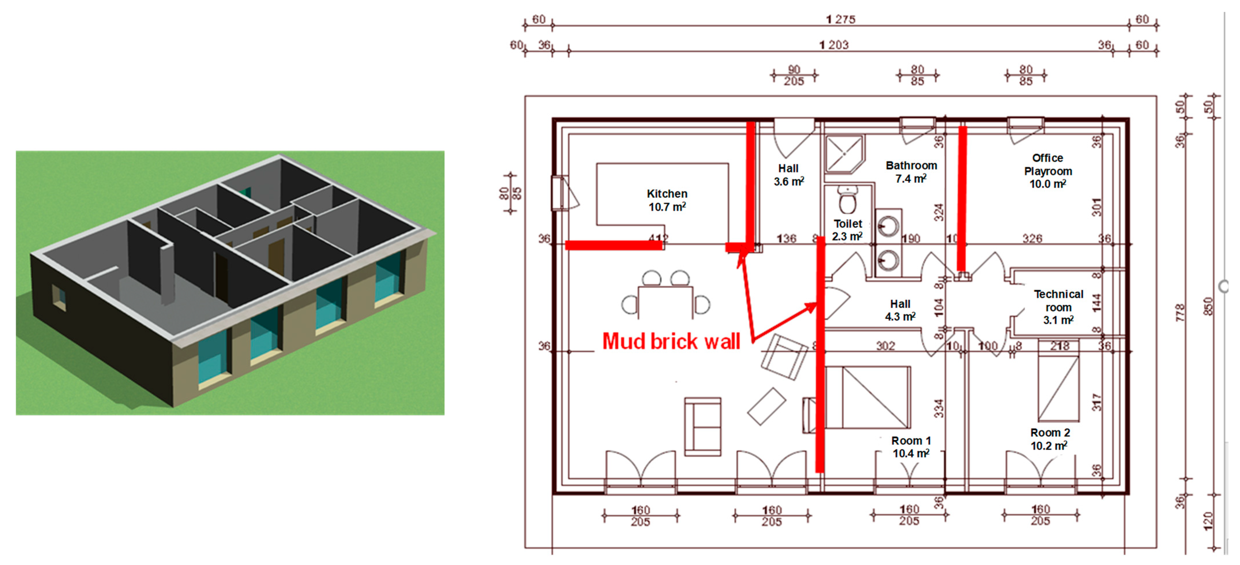
2.1. Description of the Simulated Dwelling

This study pertains to a T4-type house, on which Dynamic Thermal Simulations (DTS) were carried out using the Pleiades-Comfie software 3.2.7.1. The envelope design of this house is compatible with the requirements of RT 2012 (see Figure 1). The entire envelope and location data have been detailed in [20].

To assess the water-buffering effect of the earth wall, two types of partition walls have been compared (Figure 1):

• In the so-called “basic” version, all partition walls in the dwelling are lightweight plasterboard walls on a metal frame. The cladding on all walls is considered to be vapor impermeable; also, the hygroscopic properties of the furnishings and textiles in the home are neglected.
• In the “earth” version, the earth brick wall replaces certain partition walls over a surface area of 30.8 m², with the other assumptions remaining identical to the basic version.

The origin and characteristics (physicochemical, mineralogical, and microstructural) of the bricks used in this study are described in [21].

To determine the capacity of these two walls to regulate the environment, the indoor temperature evolution given by the DTS was used as input data for the boundary conditions of the finite element wall model (Figure 2).

The scenario for occupancy and use of the dwelling corresponds to a family of 4 and reproduces the standard routine for a work week throughout the year, as defined in the Th-BCE rules of RT2012 [22]. The steam production scenario takes into account the occupants’ metabolism and steam emissions from various domestic activities (cooking, washing, drying clothes, etc.).

Table 1. Daily steam production.

Type of Input	Amount of Water Vapor
Occupant	4 persons, 40 g/h/person (at rest), 60 g/h/person (during activity)
Kitchen	1 kg/meal, 0.5 kg/breakfast
Toilet, showers	0.5 kg in the morning, 1 kg in the evening
Washing and drying/laundry	2 kg/day, distributed between 7 a.m. and 5 p.m.

and Figure 3 summarize the daily steam production vs. day of the week input into the numerical simulation. The heating temperature set-point scenario accounts for intermittent heating during unoccupied hours. The dwelling is not air-conditioned in the summer. The ventilation scenario applied corresponds to constant airflow ventilation (CAV) with a manual low/high flow switch in the kitchen. Flow rates comply with the regulatory values listed in the 1982 decree. Not taken into account herein are infiltration, nighttime over-ventilation, and window openings.

2.2. Numerical Model

2.2.1. State-of-the-Art

The various basic models of coupled heat and mass transfer found in the literature can be grouped into two types of approaches: a homogenization approach (microscopic-macroscopic change of scale) [23,24,25,26], and a macroscopic phenomenological approach.

Generally speaking, the modeling of coupled heat, air, and moisture transfers in building envelopes is based on a phenomenological approach inspired by the work of Luikov [27]. According to this approach, the porous medium is considered to be homogeneous, which serves to establish the hygrothermal transfer equations on the basis of the fundamental principles of thermodynamics [28]. The energy and mass balances are expressed using flows derived from measurable potentials (temperature, water content, vapor pressure, relative humidity, etc.) and coefficients linked explicitly to the macroscopic properties of the materials, in particular thermal conductivity, specific heat, water vapor permeability, adsorption, and desorption properties.

Macroscopic hygrothermal transfer models are typically distinguished by the choice among the various transfer driving mechanisms used. For heat transfer, temperature is considered the standard transfer potential. For mass transfer, however, no unanimity exists; several models drive the water transfer differently. The choice and impact of water potential on the accuracy of results were discussed in the work by Janssen [29]. The author concluded that this choice depends mainly on both the level of stress applied to the material and the imposed boundary conditions. Numerous models have been established with relative humidity, including the model by Medejelekh et al. [30], developed in the GC2D Laboratory. Künzel’s model can be cited as the basis for the WUFI code [31], which is one of the most widely used commercial tools for the 1D and 2D modeling of heat and moisture transfer. The development of this model was based on the use of two drivers as potential for moisture migration, namely capillary pressure for the liquid phase and relative humidity for the gaseous phase. In the same vein, Pedersen [32] decomposed the water transfer equation into two transport equations, using vapor pressure for the vapor phase and capillary pressure for the liquid phase as the driving forces. This decomposition was carried out in order to ensure a certain continuity of capillary transfer for multilayer wall components. Other authors have used moisture content as the driving force for mass transfer. The most classical model is that of Philip et al. [33]. Similarly, Qin et al. [34] produced a non-isothermal model in which temperature and water content are considered to drive the hygrothermal transfer. During their developmental work, the authors introduced a non-isothermal diffusion coefficient, which was evaluated experimentally by quantifying the effect of the thermal gradient on moisture transfer [35]. Many other software packages are available to model coupled heat, air, and moisture transfers. For a more complete review of the state-of-the-art, Annex 41 issued by the IEA (International Energy Agency) lists most of the models existing in the literature, as well as a comparison of numerical and experimental results derived from experimental cell monitoring.

Moreover, little work in the literature has focused on coupled hygro-thermo-mechanical models; some authors have introduced coupled hygro-thermo-mechanical models to analyze the expansion of concrete [36] or wood [37]. However, nothing can be found for earthen construction materials. These models are based on a law relating the strain tensor to the stress tensor, in accordance with Equation (1).

$$\mathsf{\sigma }=\left[\mathrm{D}\right]\times \mathsf{\epsilon }=\left[\mathrm{D}\right]\times \left({\mathsf{\epsilon }}_{\mathrm{a}\mathrm{p}\mathrm{p}}+{\mathsf{\epsilon }}_{\mathrm{h}\mathrm{y}\mathrm{g}}+{\mathsf{\epsilon }}_{\mathrm{t}\mathrm{h}}\right)$$

(1)

where [D] denotes the stiffness matrix of the material, ε_app the apparent deformation of the material, and ε_hyg and ε_th the eigenstrain to hydric and thermal expansion, respectively.

The water expansion tensor is defined as a function of both the coefficient of water expansion and the moisture content of the material. The thermal expansion tensor is similarly defined. These models make it possible to accurately predict the onset of pathologies linked to dimensional variations [38]. Gonzalez proposed a more simplistic approach [39]: the stress exerted by water on the solid matrix for the various wetting and drying cycles is determined by Equation (2).

$$\mathsf{\sigma }\left(\mathrm{w}\right)=\pm \frac{{\mathrm{E}}_{\mathrm{l}}\times \mathsf{\epsilon }}{1-\mathsf{\nu }}$$

(2)

where E_l is the elasticity modulus, ε the thermal- or hydric-induced deformation, and ν the Poisson’s ratio (defined as a function of the material water content).

The pathology indicator is determined by criteria imposed on both the tensile and compressive stresses. During the drying phase, disorders arise when the computed stress is greater than the tensile strength of the dry material. Conversely, during the wetting phase, pathologies appear when the stress exceeds the compressive strength of the material.

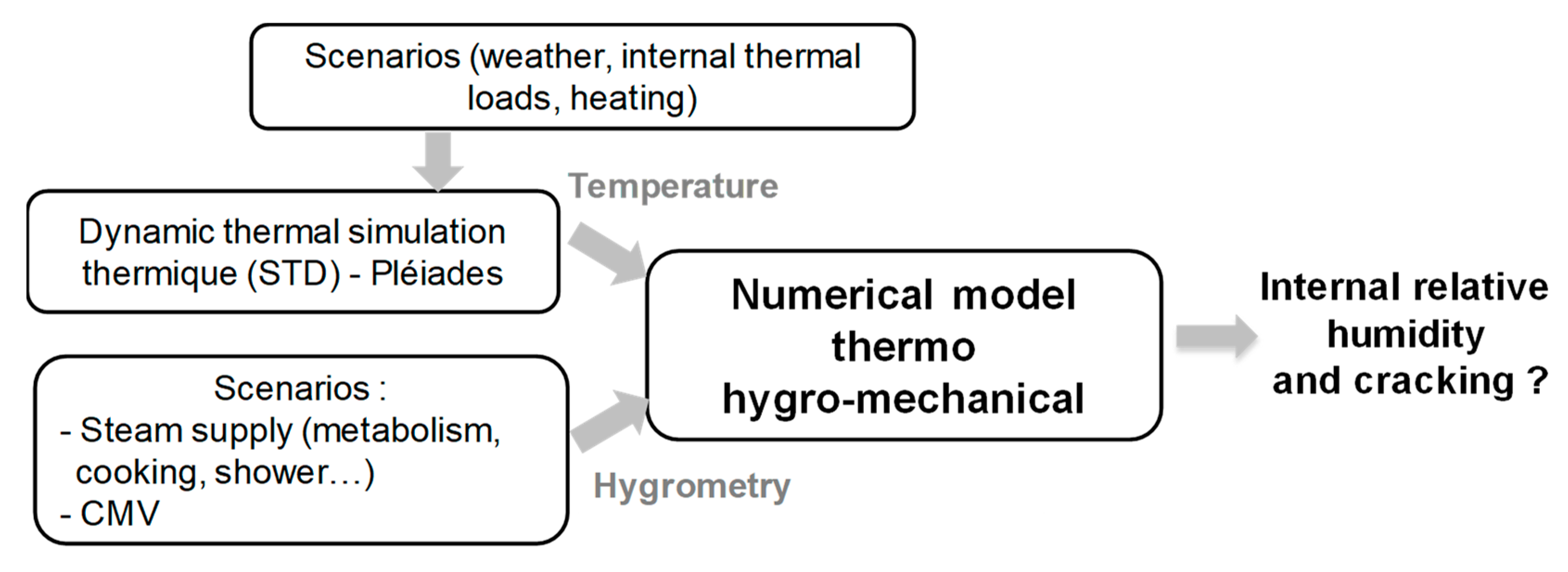
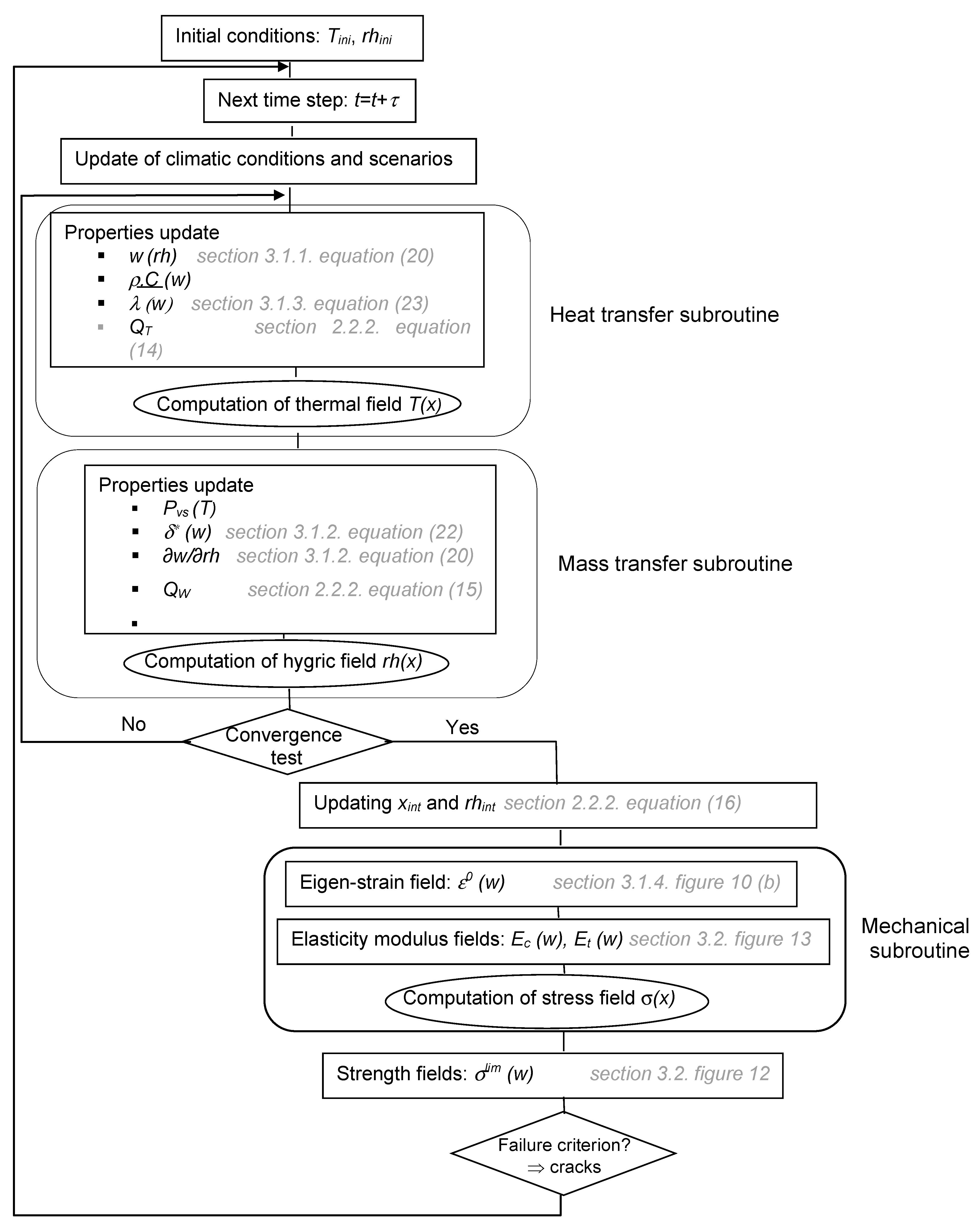
2.2.2. Description of the Numerical Model Developed

In a wall made of porous material, diffusion mechanisms can take place in three modes: heat transfer, water transfer in the liquid phase, and water transfer in the vapor phase. The simulation of these transfers within the model developed was based on phenomenological modeling approaches inspired by the work of Luikov [27]. This approach, which has been adopted for the model in the present study, considers the porous medium to be homogeneous, thus making it possible to construct the hygrothermal transfer equations on the basis of the fundamental principles of thermodynamics [27]. The phenomenological laws governing diffusion transfer are expressed as follows.

The heat transfer equation is explained by Fourier’s law, as given below:

$${\overrightarrow{\mathsf{\phi }}}_{\mathrm{T}}=-\mathsf{\lambda }\times \overrightarrow{\nabla \mathrm{T}}$$

(3)

where ${\phi }_T$ is the surface density of heat flux due to conduction [W × m⁻²], λ the thermal conductivity [W × m⁻¹ × K⁻¹], and $\overrightarrow{\nabla }\mathrm{T}$ the temperature gradient [K × m⁻¹].

The mass transfer equation is used to express the total moisture flux, as defined according to Equation (4).

$$\overrightarrow{{\mathsf{\phi }}_{\mathrm{w}}}=\overrightarrow{{\mathsf{\phi }}_{\mathrm{v}\mathrm{w}}}+\overrightarrow{{\mathsf{\phi }}_{\mathrm{l}\mathrm{w}}}$$

(4)

where φ_w is the global moisture flow density and φ_vw, φ_lw the respective surface densities of vapor flux and liquid flux [kg × m⁻² × s⁻¹]. These flows are described by Fick’s Law.

In the vapor phase, the density of vapor flow, assuming that moist air is a perfect gas, is given by Equation (5).

$$\overrightarrow{{\mathsf{\phi }}_{\mathrm{v}\mathrm{w}}}=-\mathsf{\delta }\times \overrightarrow{\nabla {\mathrm{p}}_{\mathrm{v}}}$$

(5)

where δ is the vapor permeability of the material [kg × s⁻¹ × m⁻¹ × Pa⁻¹] and $\overrightarrow{\nabla }{\mathrm{p}}_{\mathrm{v}}$ the vapor pressure gradient [Pa] adopted as a potential for this kind of transfer.

In the liquid phase, the density of liquid flow is assumed to be dependent on the gradient of moisture content. Equation (6) expresses this dependence.

$$\overrightarrow{{\mathsf{\phi }}_{\mathrm{l}\mathrm{w}}}=-{\mathsf{\rho }}_0\times {\mathrm{D}}_{\mathrm{w}}\times \overrightarrow{\nabla \mathrm{w}}$$

(6)

where ρ₀ is the material’s anhydrous density [kg × m⁻³], $D_w$ the liquid diffusion coefficient [m² × s⁻¹], and $\overrightarrow{\mathit{\nabla }}w$ the moisture content gradient [m⁻¹].

The coupled equations of the diffusion model have been expressed using a measurable transfer driving mode. Temperature T [K] is used as the potential for heat transfer, while relative humidity, denoted rh, is used for moisture transfer.

By choosing relative humidity as the only potential for water diffusion, the vapor flux density equation (Equation (5)) can be developed in the form of Equation (7), with rh = p_v/p_vs corresponding to the ratio of vapor pressure pv to saturation vapor pressure p_vs.

$$\overrightarrow{{\mathsf{\phi }}_{\mathrm{v}\mathrm{w}}}=-\mathsf{\delta }\times {\mathrm{p}}_{\mathrm{v}\mathrm{s}}\times \overrightarrow{\nabla }\mathrm{r}\mathrm{h}-\mathsf{\delta }\times \mathrm{r}\mathrm{h}\times \overrightarrow{\nabla }{\mathrm{p}}_{\mathrm{v}\mathrm{s}}$$

(7)

The liquid flux density equation (Equation (6)) is written as follows (Equation (8)) in order to keep relative humidity as the only water potential.

$$\overrightarrow{{\mathsf{\phi }}_{\mathrm{l}\mathrm{w}}}=-{\mathsf{\rho }}_0\times {\mathrm{D}}_{\mathrm{w}}\times \frac{\partial \mathrm{w}}{\partial \mathrm{r}\mathrm{h}}\times \overrightarrow{\nabla \mathrm{r}\mathrm{h}}$$

(8)

where the $\frac{\partial \mathrm{w}}{\partial \mathrm{r}\mathrm{h}}$ term is the moisture capacity resulting from the derivative of sorption isotherms.

Lastly, the derivatives of rh and p_vs allow the expression of the global moisture flow density according to Equation (9).

$$\overrightarrow{{\mathsf{\phi }}_{\mathrm{w}}}=\overrightarrow{{\mathsf{\phi }}_{\mathrm{v}\mathrm{w}}}+\overrightarrow{{\mathsf{\phi }}_{\mathrm{l}\mathrm{w}}}=-{\mathsf{\delta }}^{\mathrm{*}}\times {\mathrm{p}}_{\mathrm{v}\mathrm{s}}\times \overrightarrow{\nabla }\mathrm{r}\mathrm{h}-\mathsf{\delta }\times \mathrm{r}\mathrm{h}\times \overrightarrow{\nabla }{\mathrm{p}}_{\mathrm{v}\mathrm{s}}$$

(9)

In this equation, a unique potential (rh) is used for global isothermal moisture diffusion. A new parameter, δ*, defined as apparent vapor permeability, takes into account vapor and adsorbed liquid film as diffusion vectors within the hygroscopic domain. This variable, δ*, needs experimental determination. It is highly dependent on w. Equation (10) defines δ*.

$${\mathsf{\delta }}^{\mathrm{*}}=\mathsf{\delta }+\frac{{\mathsf{\rho }}_{\mathrm{s}}\times {\mathrm{D}}_{\mathrm{w}}}{{\mathrm{p}}_{\mathrm{v}\mathrm{s}}}\times \frac{\partial \mathrm{w}}{\partial \mathrm{r}\mathrm{h}}$$

(10)

The apparent vapor permeability has been identified over the majority of the hygroscopic range (0% < rh < 95%) by means of an inverse analysis of the sorption step kinetics. The equation used assumes the form of Equation (11).

$${\mathsf{\delta }}^{\mathrm{*}}={\mathsf{\delta }}_0\times \exp \left(\mathrm{k}\times \mathrm{w}\right)$$

(11)

where δ₀ is the vapor permeability of the material in the dry state and k is the non-linearity coefficient.

Heat and mass transfer are coupled through two balance equations. Generally, a 3D form (for heat and moisture transfer) is chosen (Equations (12) and (13) respectively).

$$\left(\overline{\mathsf{\rho }\times \mathrm{C}}\right)\times \frac{\partial \mathrm{T}}{\partial \mathrm{t}}=\stackrel{⃑}{\nabla }\left(\mathsf{\lambda }\times \stackrel{⃑}{\nabla }\mathrm{T}\right)+{\mathrm{Q}}_{\mathrm{T}}$$

(12)

$$\left({\mathsf{\rho }}_{\mathrm{s}}\times \frac{\partial \mathrm{w}}{\partial \mathrm{r}\mathrm{h}}\right)\times \frac{\partial \mathrm{r}\mathrm{h}}{\partial \mathrm{t}}=\stackrel{⃑}{\nabla }\left({\mathsf{\delta }}^{\mathrm{*}}\times {\mathrm{p}}_{\mathrm{v}\mathrm{s}}\times \stackrel{⃑}{\nabla }\mathrm{r}\mathrm{h}\right)+{\mathrm{Q}}_{\mathrm{w}}$$

(13)

where λ is the thermal conductivity [W·m⁻¹ × K⁻¹], δ* the apparent vapor permeability [kg × s⁻¹ × m⁻¹ × Pa⁻¹], ${\mathsf{\rho }}_{\mathrm{s}}$ the dry density [kg·m⁻³], and $\frac{\partial w}{\partial rh}$ the moisture capacity resulting from the derivative of sorption isotherms. The term $\left(\overline{\rho ·C}\right)$ represents the volumetric heat capacity of the wet material [J × m⁻³ × K⁻¹], which depends on the moisture content w.

Equations (12) and (13) contain two volume source terms, which form the basis of the coupling between heat and mass transfer. Their expressions are presented in Equations (14) and (15).

$${\mathrm{Q}}_{\mathrm{T}}=\mathrm{L}\times \stackrel{⃑}{\nabla }\left(\mathsf{\delta }\times \stackrel{⃑}{\nabla }\left(\mathrm{r}\mathrm{h}\times {\mathrm{p}}_{\mathrm{v}\mathrm{s}}\right)\right)$$

(14)

$${\mathrm{Q}}_{\mathrm{w}}=\stackrel{⃑}{\nabla }\left(\mathsf{\delta }\times \mathrm{r}\mathrm{h}\times \stackrel{⃑}{\nabla }{\mathrm{p}}_{\mathrm{v}\mathrm{s}}\right)$$

(15)

where ${\mathrm{Q}}_{\mathrm{T}}$ represents the contribution of the heat of sorption to the thermal balance, while ${\mathrm{Q}}_{\mathrm{w}}$ represents the influence of a thermal gradient on mass transfer in the vapor phase via the variation in saturation vapor pressure. δ is the vapor permeability [kg × s⁻¹ × m⁻¹ × Pa⁻¹] and L is the latent heat of sorption (L = 2500 kJ × kg⁻¹).

As explained in Section 2.1, the ambient relative humidity is an unknown that can be determined by a balance equation on the humidity of the area. The evolution of specific ambient humidity is calculated step-by-step from a water balance equation for air in the zone [Equation (16)].

$${\mathrm{x}}_{\mathrm{i}\mathrm{n}\mathrm{t}}^{\mathrm{t}+\tau }={\mathrm{x}}_{\mathrm{i}\mathrm{n}\mathrm{t}}^{\mathrm{t}}+\frac{\tau }{{\mathsf{\rho }}_{\mathrm{a}}.{\mathrm{V}}_{\mathrm{i}\mathrm{n}\mathrm{t}}}\left({\mathsf{\varphi }}_{\mathrm{i}\mathrm{n}\mathrm{t}}+{\mathsf{\varphi }}_{\mathrm{v}\mathrm{e}\mathrm{n}\mathrm{t}}+{\mathsf{\varphi }}_{\mathrm{w}}\right)$$

(16)

• ${\mathrm{x}}_{\mathrm{i}\mathrm{n}\mathrm{t}}^{\mathrm{t}}$ : specific humidity of the indoor air at time t [kg _water/kg _{dry air}]
• ${\mathrm{x}}_{\mathrm{i}\mathrm{n}\mathrm{t}}^{\mathrm{t}+\tau }$ : specific humidity of the indoor air at time t+ζ [kg _water/kg _{dry air}]
• $\tau$ : time step [s]
• ${\mathsf{\rho }}_{\mathrm{a}}$ : dry density of indoor air (kg/m³)
• ${\mathrm{V}}_{\mathrm{i}\mathrm{n}\mathrm{t}}$ : interior volume of the zone [m³]
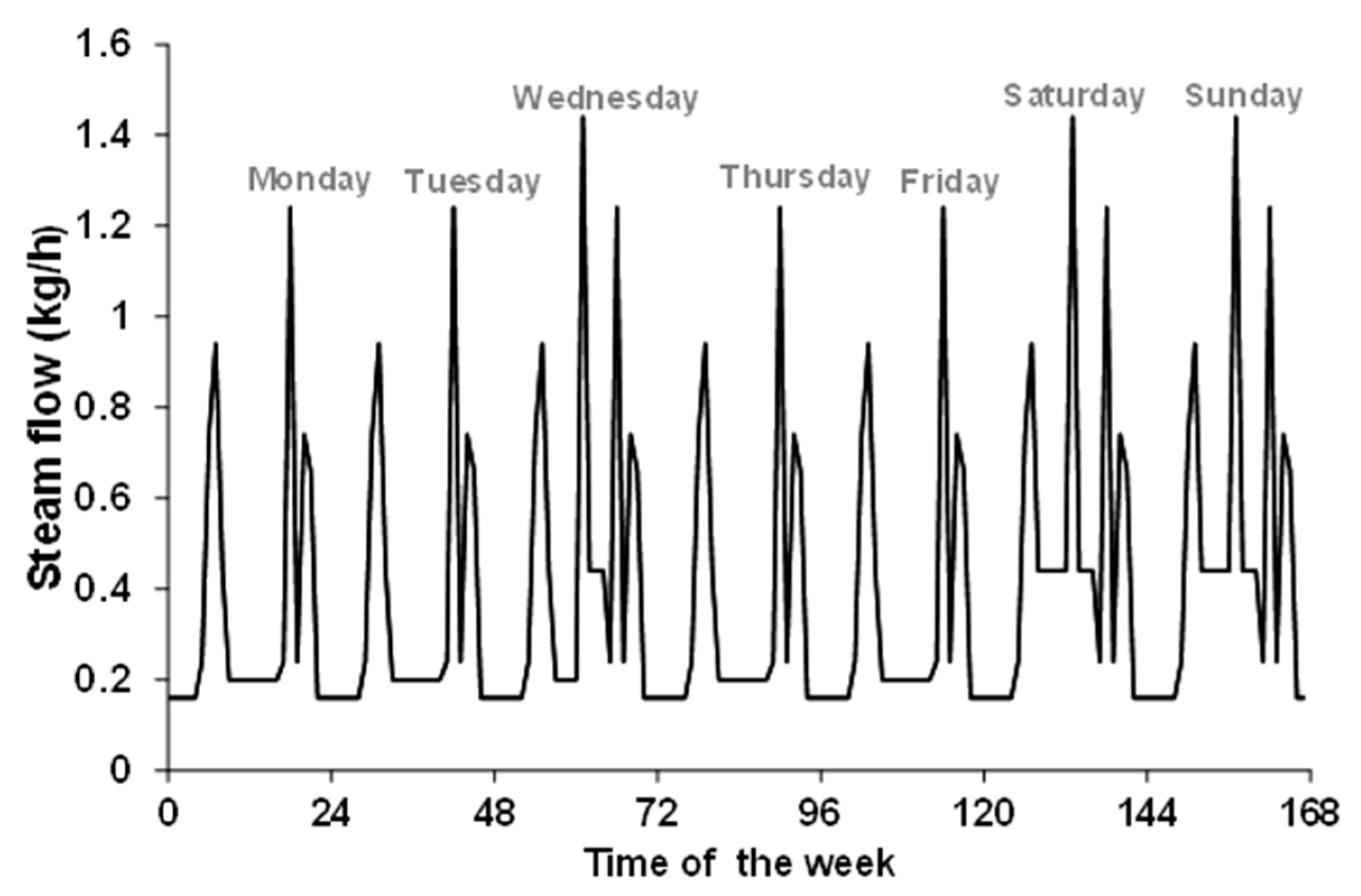
• ${\mathsf{\varphi }}_{\mathrm{i}\mathrm{n}\mathrm{t}}$ : mass flow rate of the internal water vapor inputs from occupants and processes [kg/s]
• ${\mathsf{\varphi }}_{\mathrm{v}\mathrm{e}\mathrm{n}\mathrm{t}}$ : mass flow rate of water vapor supplied by the CMV. This value is estimated using Equation (17).

$${\mathsf{\varphi }}_{\mathrm{v}\mathrm{e}\mathrm{n}\mathrm{t}}=\frac{{\mathrm{Q}}_{\mathrm{a}\mathrm{i}\mathrm{r}}}{3600}\times {\mathsf{\rho }}_{\mathrm{a}}\times \left({\mathrm{x}}_{\mathrm{e}\mathrm{x}\mathrm{t}}-{\mathrm{x}}_{\mathrm{i}\mathrm{n}\mathrm{t}}\right)$$

(17)

• ${\mathrm{Q}}_{\mathrm{a}\mathrm{i}\mathrm{r}}$: extracted air volume flow rate [m³/h]
• ${\mathrm{x}}_{\mathrm{e}\mathrm{x}\mathrm{t}}$ and ${\mathrm{x}}_{\mathrm{i}\mathrm{n}\mathrm{t}}$ : specific humidity of outdoor and indoor air [kg _water/kg _{dry air}]
• ${\mathsf{\varphi }}_{\mathrm{w}}$ : mass flow rate of water vapor transferred from the wall to the environment [kg/s]. This value is calculated according to Equation (18).

$${\mathsf{\varphi }}_{\mathrm{w}}={\mathsf{\varphi }}_{\mathrm{w}\mathrm{m}\mathrm{o}\mathrm{d}}\times \frac{{\mathrm{S}}_{\mathrm{m}\mathrm{u}\mathrm{r}}}{{\mathrm{S}}_{\mathrm{m}\mathrm{o}\mathrm{d}}}$$

(18)

• ${\mathsf{\varphi }}_{\mathrm{w}\mathrm{m}\mathrm{o}\mathrm{d}}$ : mass flow of water vapor leaving the surface S_mod of the model [kg/s]
• ${\mathrm{S}}_{\mathrm{m}\mathrm{o}\mathrm{d}}$ : exchange surface area of the model [m²]
• ${\mathrm{S}}_{\mathrm{m}\mathrm{u}\mathrm{r}}$ : total exchange surface area of the actual wall (including both faces) [m²]

After each time step, the relative humidity of the indoor air is calculated from the temperature and the new specific humidity. A time step of 300 s was implemented following a sensitivity study showing that results converged with any simulation run using a smaller time step.

2.2.3. Simulation of Coupled Behavior

Figure 4 presents the approach adopted to develop the coupled hygro-thermo-mechanical model. The algorithm was implemented in the Gibiane language within the Cast3M finite element environment [40]. The resolutions when calculating the T(x) or rh(x) fields at each time step use conventional transient thermal operators with a relaxation parameter θ = 1. The numerical processing of the coupled transfer consists of solving the thermal equation and then the water equation at each time step. This process is repeated iteratively in updating the physical properties (thermal and vapor conductivity, heat and water capacity, etc.) as well as the saturation vapor pressure and source terms after each solution. This iterative process was repeated until reaching convergence, which occurred when the variation in each unknown (temperature and humidity) between two iterations was below a given threshold. Next, the mechanical stress field generated by the shrink-swell deformations was determined for each time step and compared with both the tensile and compressive strengths obtained through experimentation to detect crack occurrence.

3. Determination of Model Input Parameters

A multidisciplinary experimental campaign was carried out on the brick in order to feed the numerical model and reproduce the phenomena of transport and storage of moisture and heat to which a wall may be subjected under real-world conditions. This study has primarily focused on analyzing the moisture content of the material and its impact on thermohydric properties. Among the many hygrometric properties measured are sorption isotherms, water capacity, and apparent permeability. Thermal properties are determined by means of thermal conductivity and thermal capacity. To estimate the deformations capable of being generated by the water field, the shrinkage/swelling coefficient as a function of content was also measured. The experimental protocols used to identify these properties will be detailed in the following section.

3.1. Characterization of Thermal and Hydric Properties

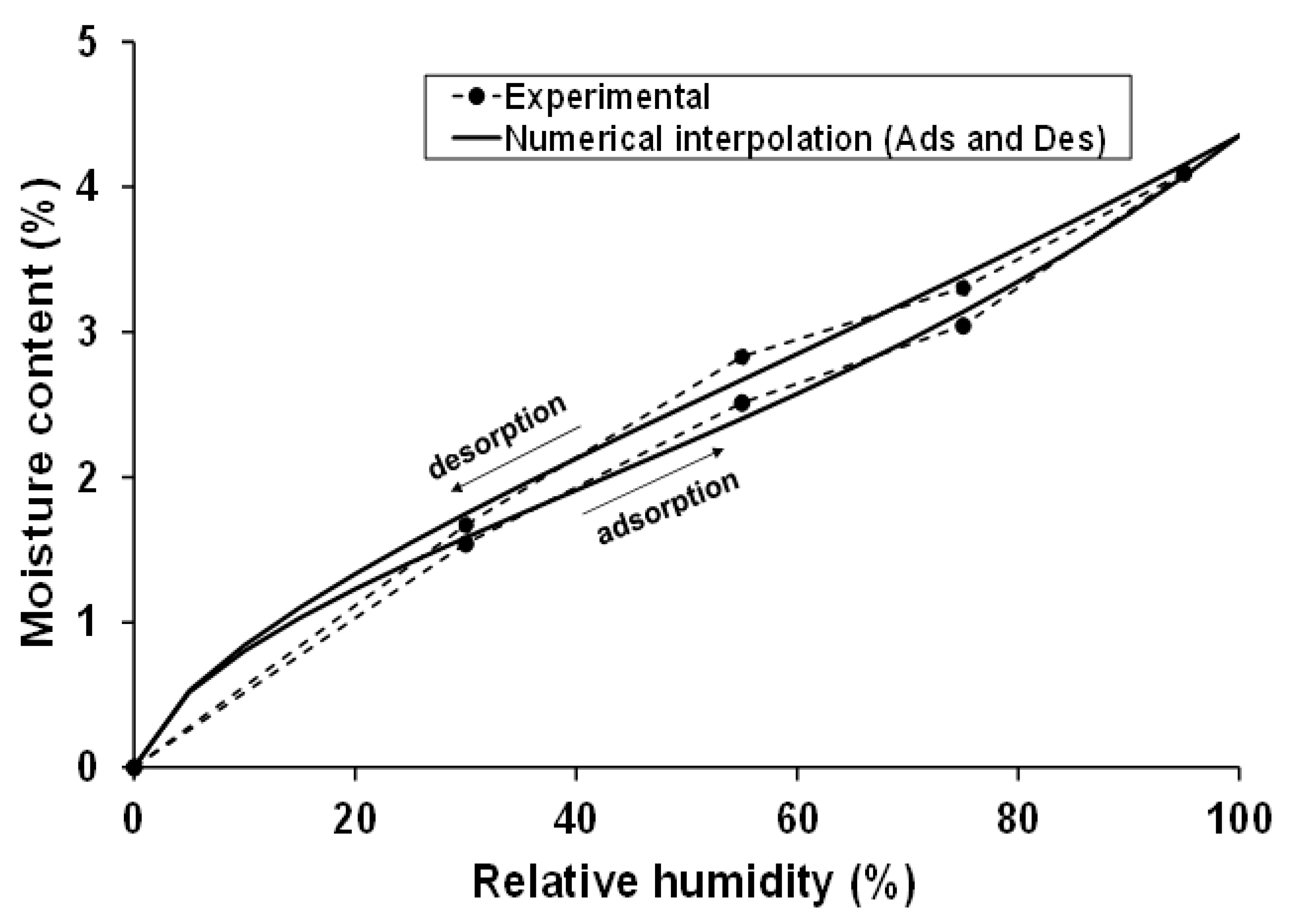
3.1.1. Sorption Isotherm and Moisture Capacity

The sorption isotherm test was conducted in strict accordance with the recommendations of Standard NF EN ISO 12571 [41]. This test entails a curve yielding the equilibrium water content of the material as a function of the relative humidity of the environment at a given temperature. To measure the sorption isotherm, the samples were first dried to a constant mass at a temperature of 105 °C, as specified in ISO NF EN ISO 12570 [42], in order to extract all physically bound water. The samples were then placed in a climate chamber, where the temperature was held constant at 23 °C and where Relative Humidity (RH) increased in successive stages (30, 55, 75, and 95% RH). The water content by mass (w) was determined for each equilibrium at each humidity level. This equilibrium could be obtained by periodically weighing the test specimens until their mass reached a constant level. Weight is considered constant once the variation in mass between three consecutive weighings performed 24 h apart drops below 0.1% of the total weight. The desorption curve is obtained in a similar way, in successive steps of decreasing relative humidity, with the starting point corresponding to the last point of the sorption curve (95% RH).

The construction of the two-branch sorption isotherms was based on the thermodynamic approach developed by Merakeb [43] [Equation (19)].

$$w\left(rh\right)=w_s\times \mathit{exp}\left({\phi }_i\times \mathit{ln}\left(rh\right)\times \mathit{exp}\left(a_i\times rh\right)\right)$$

(19)

In this equation, φ_a and φ_d are thermodynamic parameters, and a_a and a_d are calibration constants corresponding, respectively, to the adsorption (index a) and desorption (index d) phases. w_s corresponds to the equilibrium moisture content for relative humidity at saturation (100% RH). The three parameters φ_i, a_i, and w_s of each isothermal curve are identified by minimizing the differences between the theoretical curve and the measurement points by using the least squares method.

The average values of these parameters are as follows:

• Adsorption: w_s = 4.35%, a_a = 0.67, φ_a = 0.68
• Desorption: w_s = 4.35%, a_d = 0.30, φ_d = 0.69

Figure 5 shows the results of this interpolation superimposed on the experimental results.

Let us note that the model closely follows the experimental values, with a different asymptote at the beginning of the curve. This observation can be justified by the lack of experimental data over the 0–30% RH range. It should also be noted that the water content increases as a function of relative humidity, with a steeper slope towards condensation (RH > 75%). This characteristic reveals the high potential of this material to absorb and capture moisture. In addition, a comparison of the adsorption and desorption curves shows the existence of a slightly open hysteresis as the relative humidity increases (>55%). This finding reflects the greater ease with which water enters the porous network than leaves it, as well as differences in capillary forces during the adsorption and desorption phases and, most likely, the tortuosity of the porous network.

The moisture capacity ξ is expressed by the slope of the sorption isotherm curve; it represents the capacity of a material to store moisture within and thus characterizes the hydrous inertia of the material under isothermal conditions. This parameter is obtained from the derivative of the analytical equation for the sorption isotherm and is expressed by Equation (20).

$$\mathsf{\xi }=\frac{\partial \mathrm{w}}{\partial \mathrm{r}\mathrm{h}}=\mathrm{w}\left(\mathrm{r}\mathrm{h}\right)\times \mathsf{\phi }\times \exp \left({\mathrm{a}}_{\mathrm{i}}\times \mathrm{r}\mathrm{h}\right)\times \left(\frac{1}{\mathrm{r}\mathrm{h}}+{\mathrm{a}}_{\mathrm{i}}\times \ln \left(\mathrm{r}\mathrm{h}\right)\right) \mathrm{w}\mathrm{i}\mathrm{t}\mathrm{h} \mathrm{i}=\mathrm{a},\mathrm{d}$$

(20)

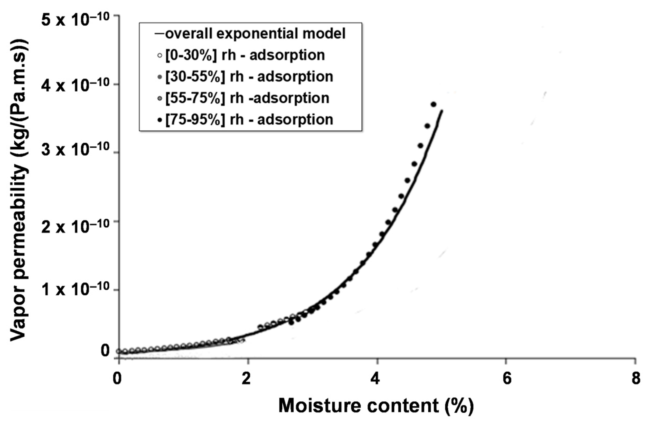
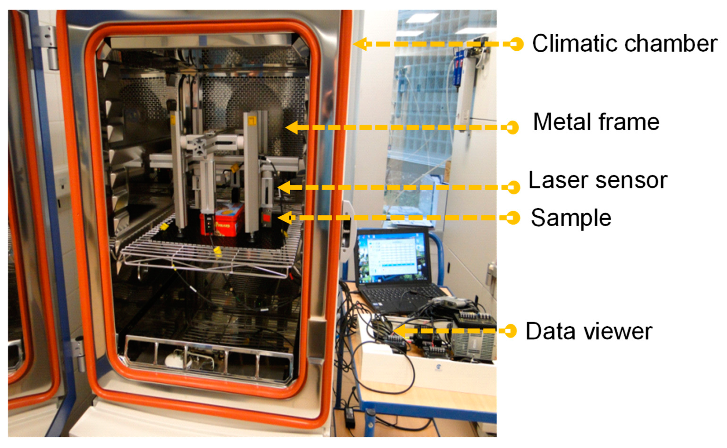
3.1.2. Apparent Vapor Permeability

The apparent permeability δ* (vapor phase + liquid phase) as a function of water content was identified by means of the inverse (simplex) method by utilizing the sorption kinetics of the transient phases until the various steps had been completed. The sorption steps were simulated by the hygrothermal transfer model developed at GC2D in the CAST3M finite element environment [44]. The goal of solving the inverse problem is to derive unknown characteristics from the measured data. Parametric identification was based on minimizing the differences between theoretical and measured changes in mean water content.

According to preliminary research [45], it is possible to fit the apparent vapor permeability to an exponential law defined in Equation (21).

$${\mathsf{\delta }}^{\mathrm{*}}={\mathsf{\delta }}_0\times \exp \left(\mathrm{k}\times \mathrm{w}\right)$$

(21)

where ${\delta }_0$ is the vapor permeability of the material in the dry state and k the non-linearity coefficient.

The identification of parameters “δ₀” and “k” relies on an optimization algorithm (simplex), which minimizes the relative difference between theoretical and measured mean water content changes. For each sorption step, the permeability values as a function of water content are determined via this approach. Figure 6 presents the geometric model and Cast3M mesh used.

All symmetry properties were used in order to reduce the computing time resulting from a tetrahedral model. This figure also provides an example of the humidity and temperature fields calculated during the adsorption phase.

The results of these identifications are plotted in Figure 7 as a set of hyperbolic segments, which correspond to the permeability calculated for each sorption step (adsorption and desorption). The continuous curve (in black) is constructed by smoothing over all segment clusters. This step allows for permeability to be modeled as a continuous law as a function of water content [Equation (22)].

$${\mathsf{\delta }}^{\mathrm{*}}=9.4\times {10}^{-12}\times \exp \left(68.4 \mathrm{w}\right)$$

(22)

This identification method is quite original in that it enables the hygroscopic nature of the material to be assessed over a wide range of relative humidity values, unlike the cup test standardized in EN ISO 12572 [46], which only delivers two discrete values: one under dry conditions (0–55% RH) and the other under wet conditions (55–100% RH), exposing a significant difference.

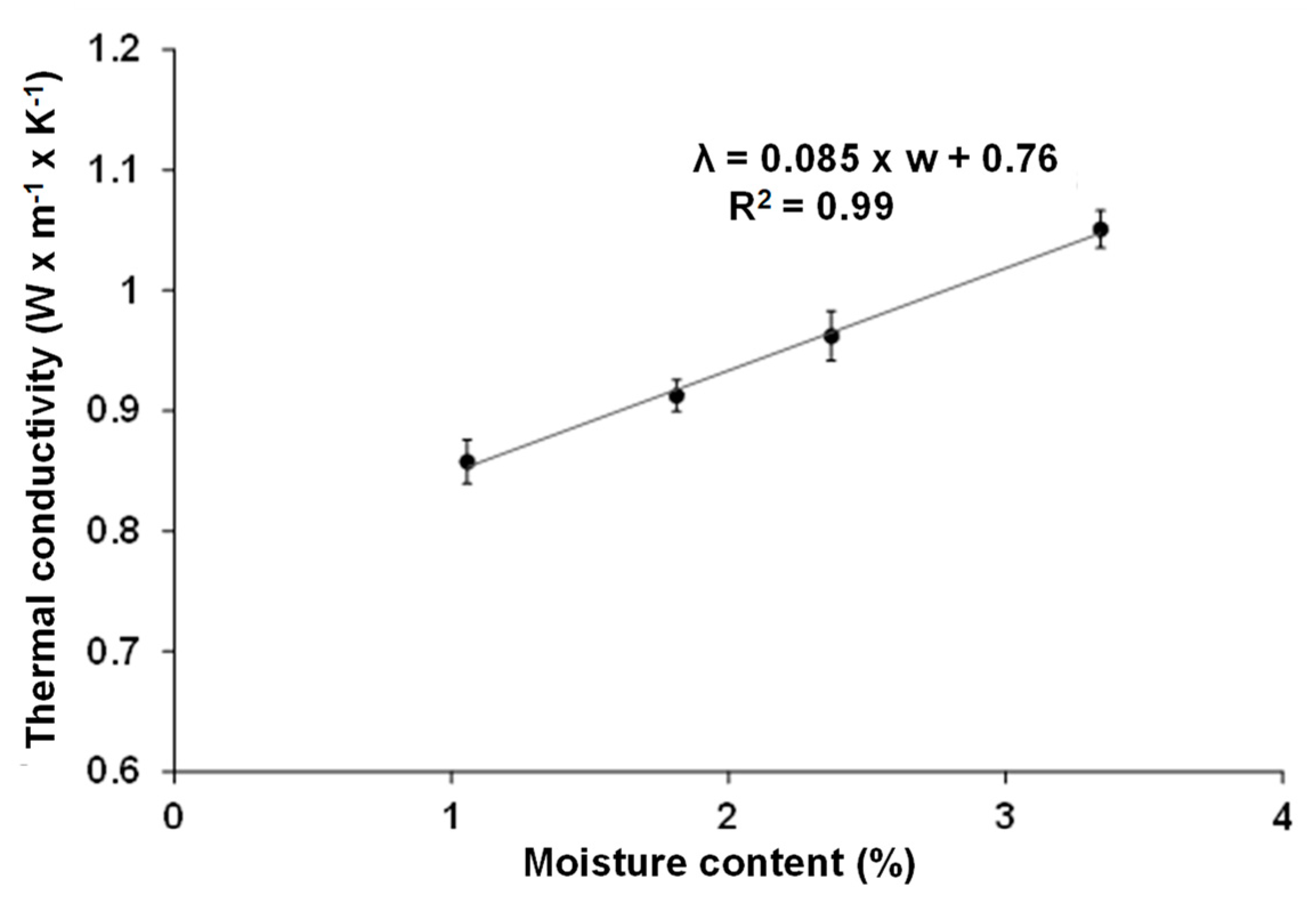
3.1.3. Thermal Conductivity

Figure 8 shows thermal conductivity values measured with the Hot Disk as a function of water content (this technique is described in detail in [20]). Each point represented in this figure corresponds to the average of six measurements, spaced one hour apart to avoid overheating the material (evaporation/condensation). Based on the results obtained, it was decided to model the evolution of thermal conductivity as a function of water content by a linear law described in Equation (23). This choice is in agreement with the data found in the literature [47,48].

$$\mathsf{\lambda }=0.085 \times \mathrm{w}+0.76 \left({\mathrm{R}}^2=0.99\right)$$

(23)

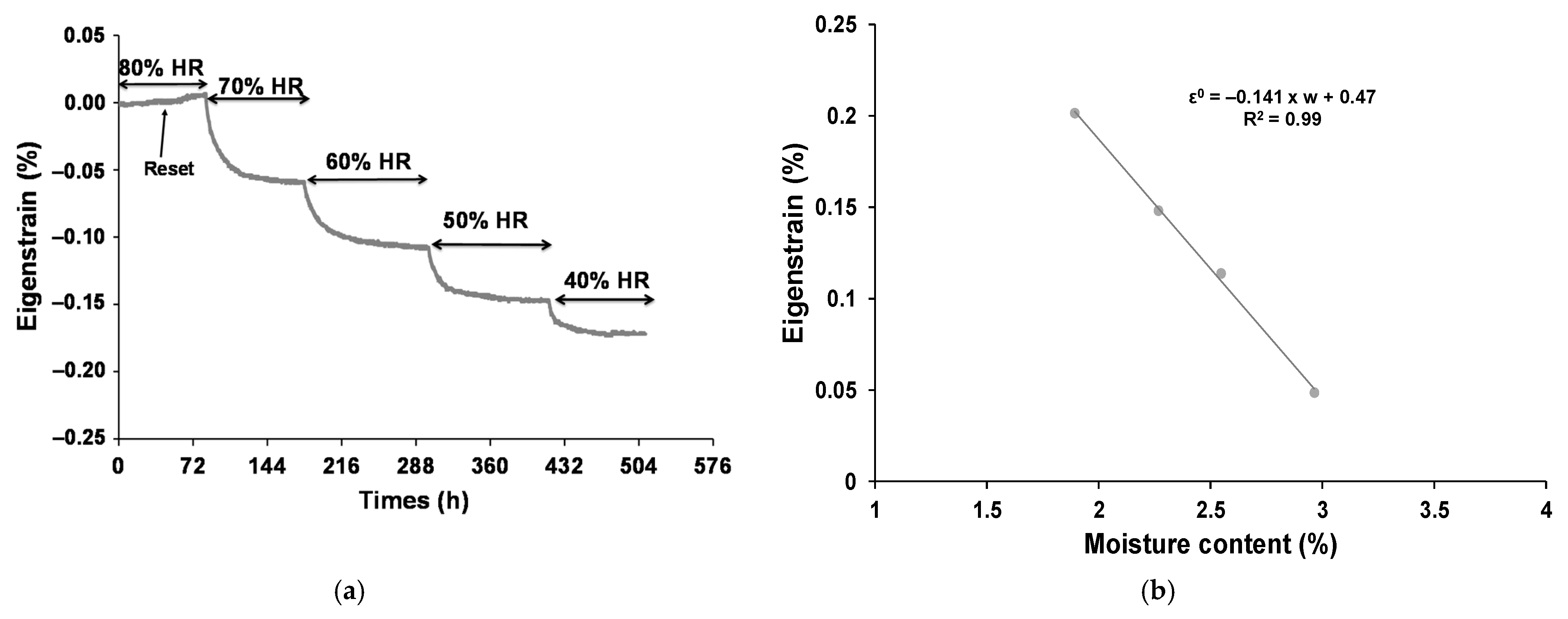
3.1.4. Calculation of the Water-Induced Eigenstrain Field

To determine the deformations of the brick generated by the water field, a climatic chamber equipped with a device for the in situ measurement of dimensional variations was employed at various relative humidity values: 80, 70, 60, 50, and 40% RH (Figure 9). This device was designed by the CTMNC [49] and comprises a set of laser source/sensor pairs fastened to a rigid frame around the sample faces. It is suitable for measuring eigenstrain materials that are highly sensitive to water, such as earth bricks. The test was carried out on an entire brick conditioned at 23 °C and initially stabilized at 80% RH.

Figure 10a,b displays the variation in deformation as a function of time at different relative humidity values, along with the shrinkage coefficient vs. water content. This coefficient, α, is calculated as the ratio of the difference in eigenstrain ε⁰ to the difference in water content between two relative humidities: α =∆ ε⁰/∆w. The results in Figure 10a demonstrate that most of the deformation occurs at high relative humidity, with greater amplitudes at the outset. This amplitude then decreases with lower relative humidity until it reaches a phase where the water evacuation rate is more or less stable. This sequence can be explained both by the clay platelets, which tighten under the effect of capillary forces as relative humidity decreases, and by porosity and granular stacking.

The evolution of the shrinkage coefficient vs. water content (Figure 10b) indicates a similar behavior, which can be modeled by a linear law. In this study, it has been considered that the shrinkage and swelling coefficients are identical, given the low hysteresis of the material. For this reason, the numerical model will be input with a coefficient equal to 0.141, which is the average value for a relative humidity lying between 80% and 40%.

3.2. Characterization of Hygro-Mechanical Properties

In order to identify the consequences of the stresses generated by shrinkage and swelling, a fracture criterion characterizing the transition from elastic to post-elastic mechanical behavior has been defined by determining the mechanical properties in tension and compression under different water stresses. The procedures and results of each test will be presented in the following sections.

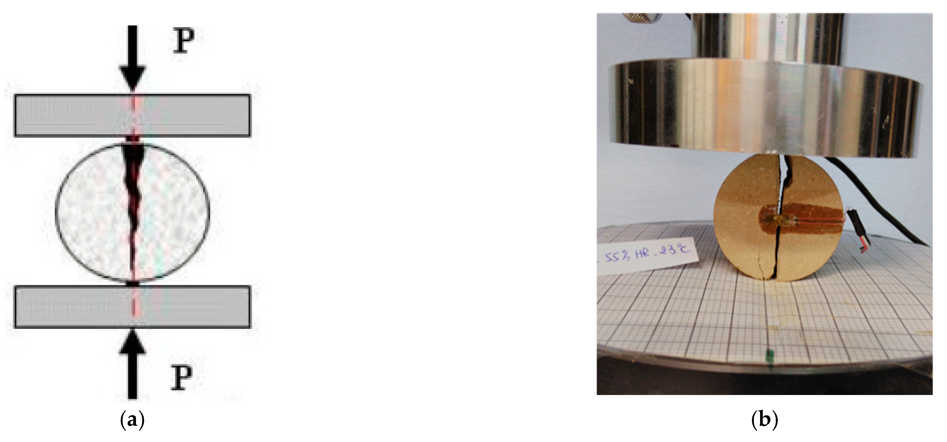
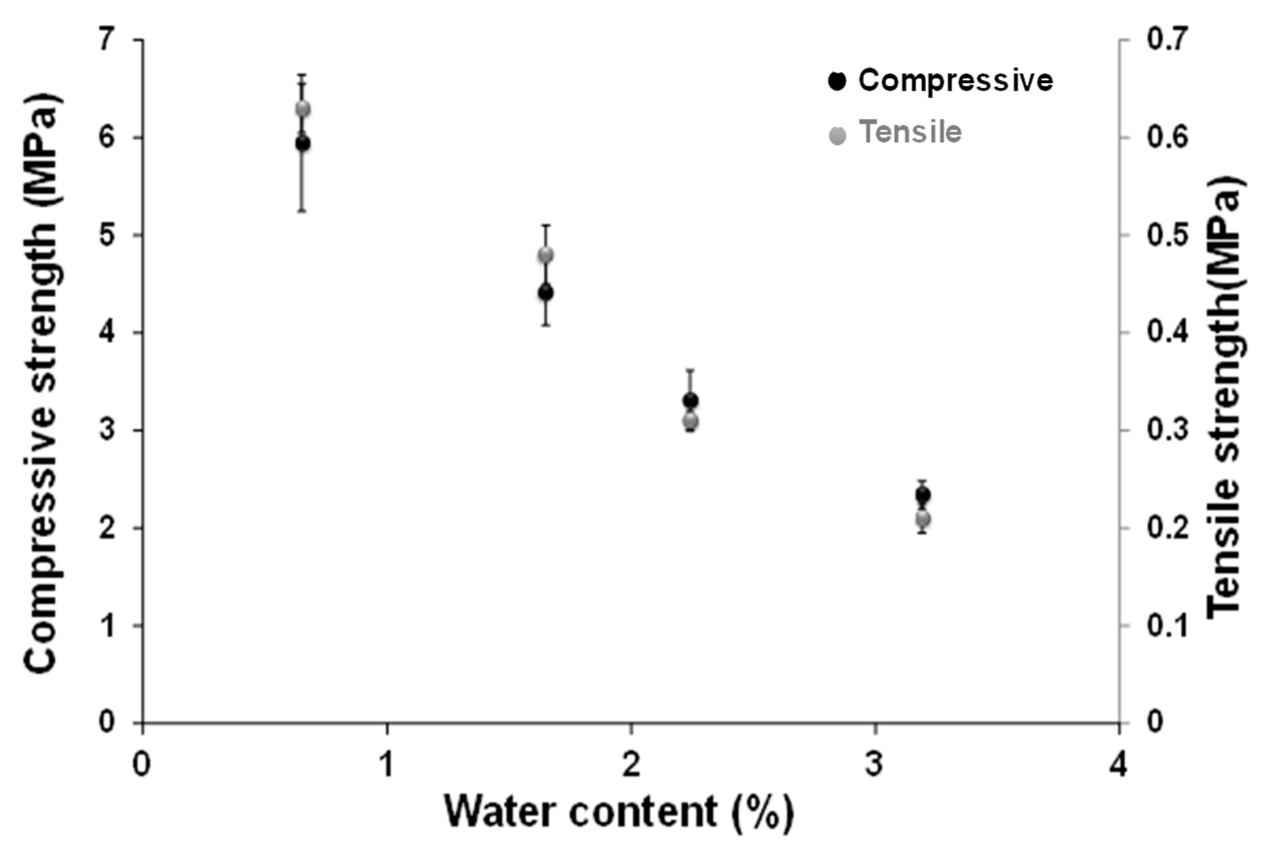
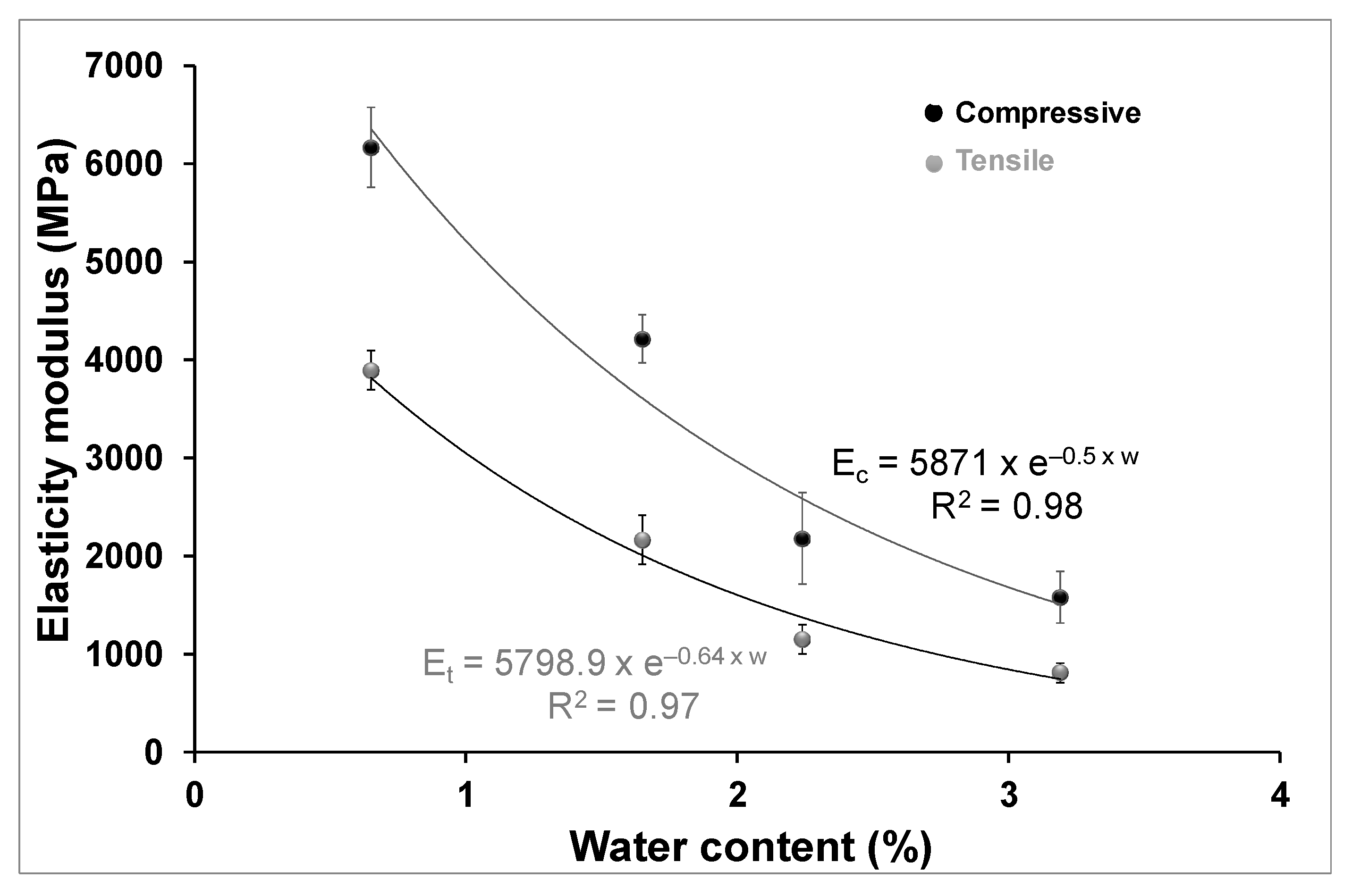
3.2.1. Compression Test

Compression tests were conducted on specimens measuring 5 × 5 × 10 cm³ using a Zwick press equipped with a 50 kN load cell whose crosshead moves at 0.5 mm/min [50]. To reduce shrinkage effects and circumferential stresses, a slenderness of two was adopted between height and length [51,52]. To establish unbiased compression test conditions, the parallelism of the specimen loading surfaces was corrected by surfacing with a commercial epoxy adhesive; moreover, a set of cardboard plates was placed on either side of the specimen. The device was glued to the compression fixture to ensure the slack was taken up. Deformation during the tests was monitored using a strain transducer with a stroke equivalent to 2.5 cm, clamped in the middle third of the test specimens away from the edges.

3.2.2. Tensile Test (Brazilian)

This test was performed in accordance with the recommendations set forth in Standard NF P94-422 [53]; it consists of compressing a cylindrical specimen along two diametrically opposed generatices (Figure 11a) at a loading speed of 0.3 mm/min. The force applied induces tensile and compressive stresses within the specimen. In theory, failure is obtained by traction along the vertical diameter, thus resulting in a vertical splitting of the specimen. The specimens tested have a slenderness equal to two and dimensions of Φ = 45 mm and h = 85 mm. To measure strain, a Vishay strain gauge was glued to the middle of the specimen (Figure 11b). The tensile stress at failure σ_t was determined using the linear elasticity assumption for isotropic materials, as described in Equation (24). Prior to mechanical testing, the specimens were conditioned at 23 °C and at different relative humidity values of 8, 30, 55, and 75%. For each humidity level, at least six specimens were tested.

$${\mathsf{\sigma }}_{\mathrm{t}}=\frac{2\times \mathrm{F}}{\mathsf{\pi }\times \mathrm{D}\times \mathrm{L}}$$

(24)

where F is the vertical force applied at failure, D is the specimen diameter, and L is the specimen length.

Figure 12 shows the peak stress values obtained in compression and tension as a function of water content. The two curves offer a similar trend, with a clear decrease in mechanical strength as water content increases. This observation is in agreement with data previously published in the literature on earth construction materials [54,55]. This decrease can be attributed not only to the decrease in suction as water content increases, a phenomenon well studied in soil mechanics [56], but also to the fact that water lubricates the contact points between the grains in the pile. An average ratio of ten can be noted between compressive and tensile strength (Brazilian), a finding consistent with the ratio measured on BTC [57].

For the modulus of elasticity (Figure 13), this same type of behavior was observed, both in compression and in tension. This observation can be explained by the water treatment, which disrupts granular stacking and therefore modifies the intensity of the physicochemical bonds between the clay platelets. As regards this particular model, it was decided to fit these data using an exponential law with a correlation coefficient of approximately 0.97.

4. Numerical Results

4.1. Annual Study

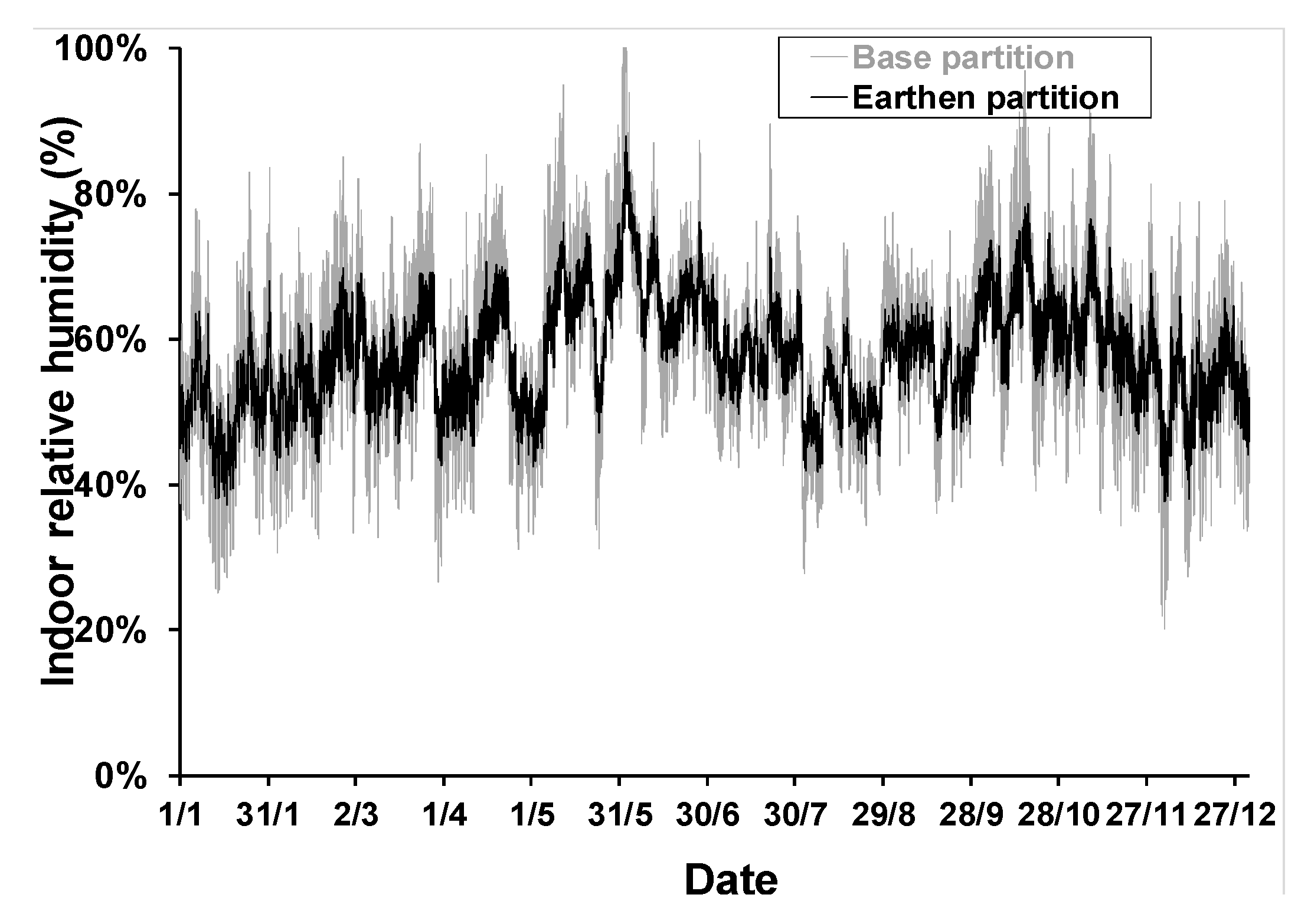
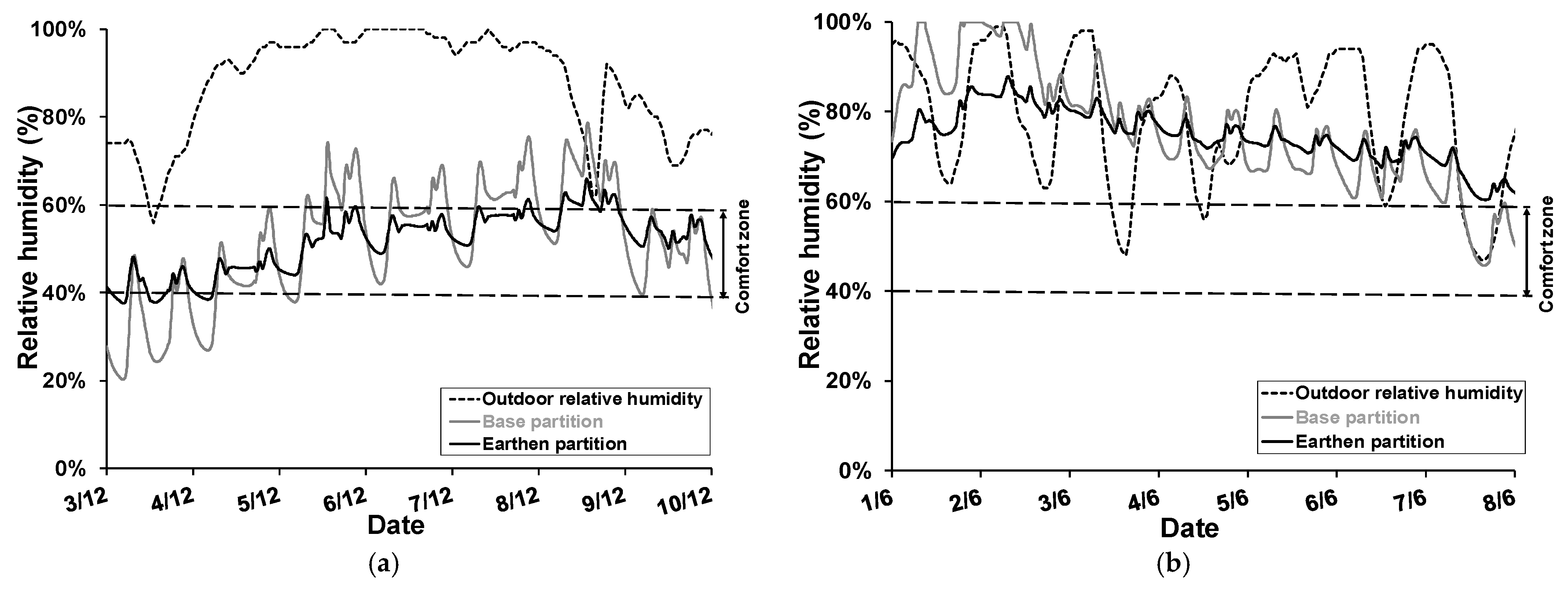
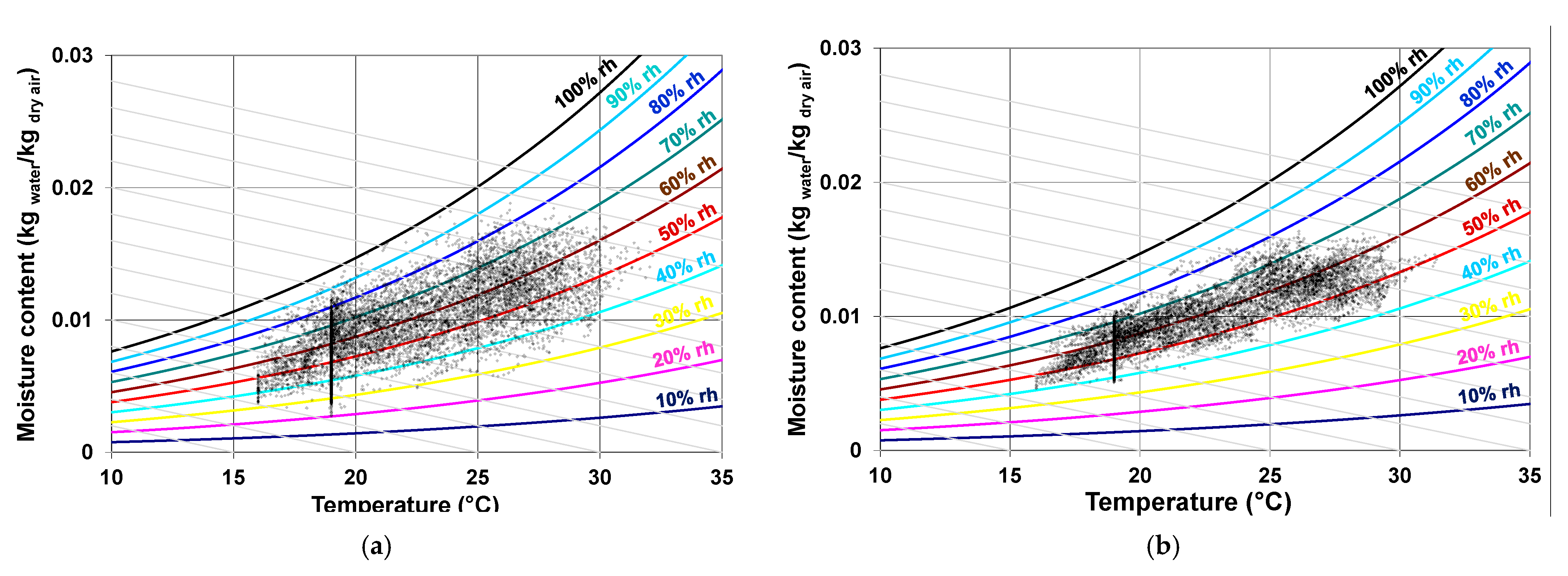
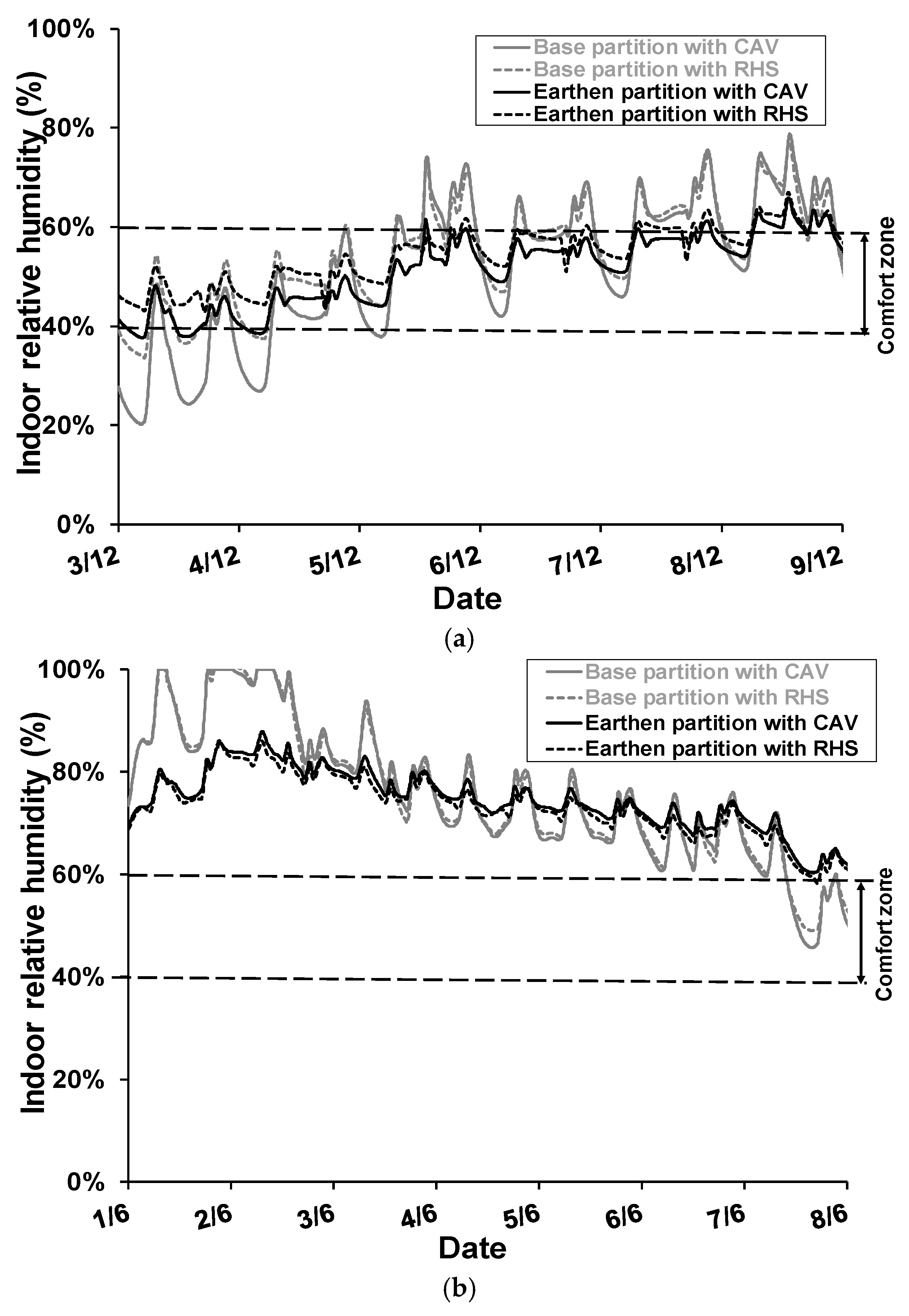
4.1.1. The Regulating Effects of Partition Walls on Indoor Humidity

Figure 14 shows the annual changes in indoor humidity when a basic partition wall and an earth partition wall are used. It can be seen from these trends that indoor humidity is strongly influenced by the nature of the partition wall, as reflected by a clear reduction in the amplitude of daily variations in the case of the earth partition wall. This behavior can be explained by the microstructure and absorbent effect of the clay contained in the brick, thus allowing water vapor to permeate until a hygroscopic equilibrium is established between the material and the air. This dynamic exchange makes it possible to maintain constant hygrometry around the optimal comfort zone of 40% to 60% RH, as defined by Givoni. It can be concluded that partition walls made with earth bricks lead to a drop in annual humidity amplitude of around 50% compared with the basic partition walls, with much lower peaks at around 45%.

Figure 15a,b portrays a close-up of two sequences corresponding, respectively, to the winter and summer behavior of the partition walls tested. The two graphs show the performance of the earth partition wall as a hygrometric balance in the case of high daily humidity.

During the winter sequence (Figure 16a), the relative humidity of the indoor air remains between 35% and 65% when earth partition walls are used, whereas the humidity of the basic partition walls varies from 20% to 75% depending on the outdoor variations, i.e., a 25% reduction on average. In this case, earth partition walls offer an average of 6% more relative humidity than the basic walls. During the summer sequence (Figure 16b), earth partition walls largely absorb the fluctuations in relative humidity compared with basic partition walls. The relative humidity remains between 56% and 87%, while that of the basic walls lies between 62% and 100%. During this period, no partition walls achieve optimal comfort conditions due to the absence of a dehumidification system that reduces humidity in the air.

The Givoni diagram (Figure 16) plots the hygrothermal conditions of indoor air on a psychrometric diagram, hour by hour, over the course of the year [58]. The vertical constriction of the point cloud clearly shows the regulating power of earth partition walls on relative humidity.

Figure 17 illustrates, for a summer week, the water flows absorbed or desorbed by the wall as compared with the vapor flow produced due to the occupancy. It can be noted that a significant proportion of this moisture is exchanged alternately by the wall, with the other part being continuously discharged by the CMV system. The earthen brick wall reacts instantaneously to any internal vapor release. These simulations therefore demonstrate the excellent efficiency of earth brick walls in terms of water regulation.

This section exposes the ability of materials to regulate humidity in indoor premises. However, the impact of the use of partition walls on humidity peaks must be placed in context with the various ventilation strategies. The following section will address this topic.

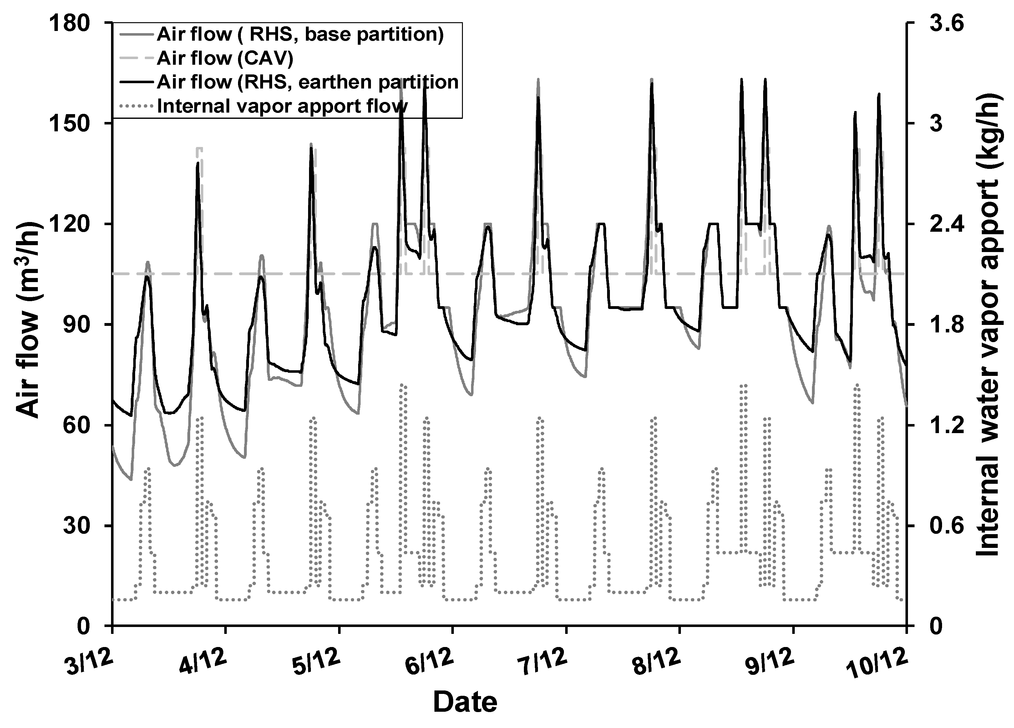
4.1.2. Impact of the Choice of Ventilation on Partition Behavior

To study the influence of earth partition walls on ventilation rates in the case of relative humidity-sensitive ventilation (RHS), it was decided to focus on the week from 3 to 9 December, which includes the day with the highest RH amplitude. This week is characterized by very cold days (around −10 °C on 3 December). For such days, the choice of humidity-sensitive ventilation avoids very low ambient humidity. This regulating effect is accentuated by the presence of earth partition walls (Figure 18a).

For the summer period, the beneficial effect of the earth wall can also be observed in the regulation of ambient relative humidity, regardless of the ventilation system in use (Figure 18b).

The optimal impact of ventilation and partitioning choices on energy requirements and, therefore, on consumption is achieved by reducing ventilation rates during the heating season. When humidity-sensitive ventilation is used, the advantage of the earth partition wall in terms of humidity control and comfort induces a negative counterpart in terms of energy consumption since the air flow rate is reduced (Figure 19). On the other hand, this finding may answer doubts regarding the use of humidity-controlled ventilation, which is blamed for a high level of pollutants due to the lack of ventilation during the winter.

From an energy perspective, earth bricks have little impact, or even a slightly negative impact, in the presence of RHS ventilation. In all cases, the internal water vapor produced must be discharged at some point by the CMV; the brick combined with a humidity-sensitive system merely delays the change in airflow. It could not be clearly demonstrated that the brick reduced the airflow at the coldest times of day, with compensation from its increase at the hottest times. Moreover, this little or slightly negative impact is due to the fact that earth bricks increase the lowest values of air flow. These conclusions are in agreement with those stated by Kwiatkowski et al. [59], who compared the effects of non-hygroscopic and moisture-buffering gypsum walls for both ventilation systems. In our specific case, a dynamic simulation model, truly coupled with the hygrothermal model, would enable more rigorous conclusions to be drawn [49].

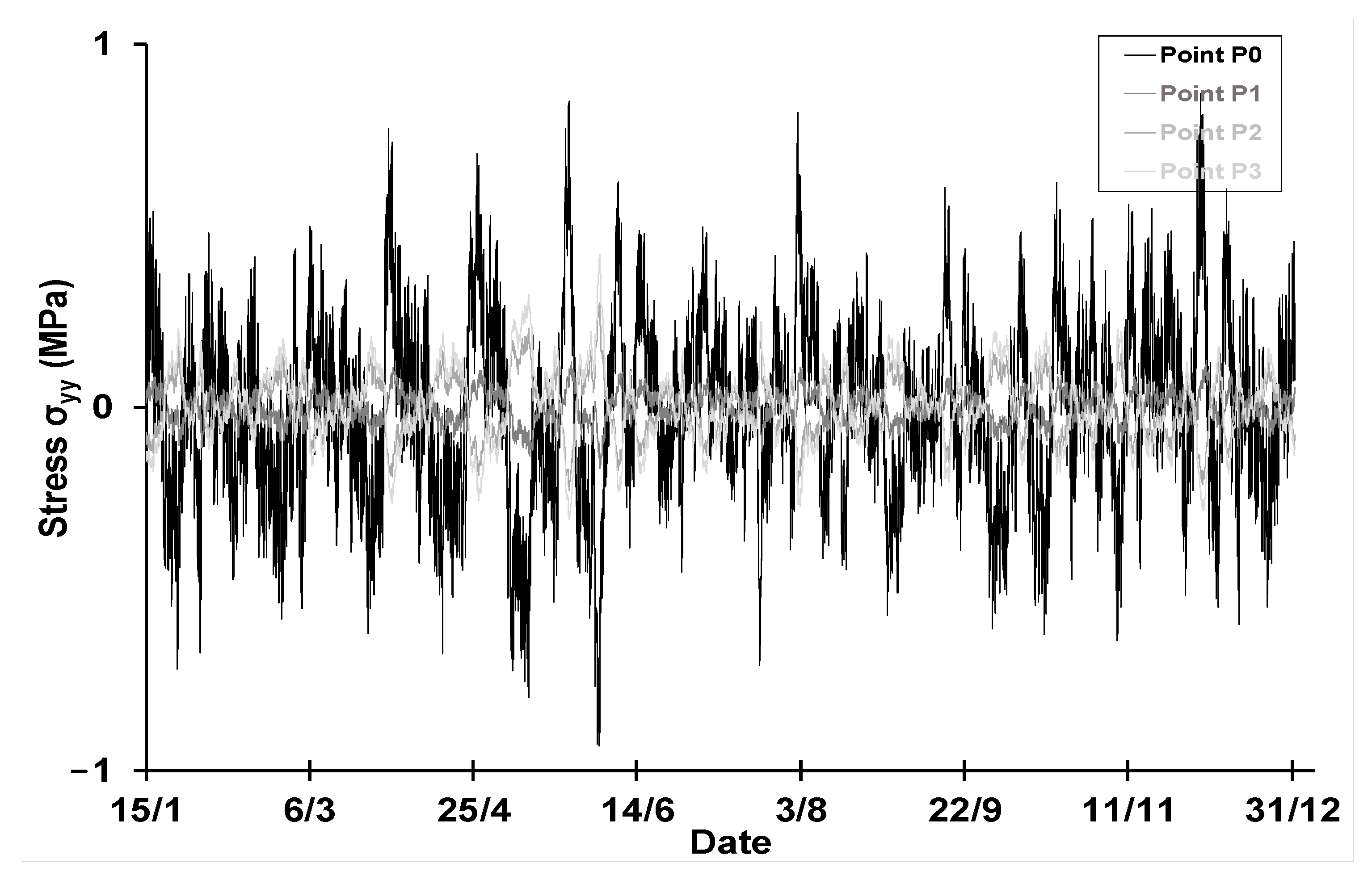
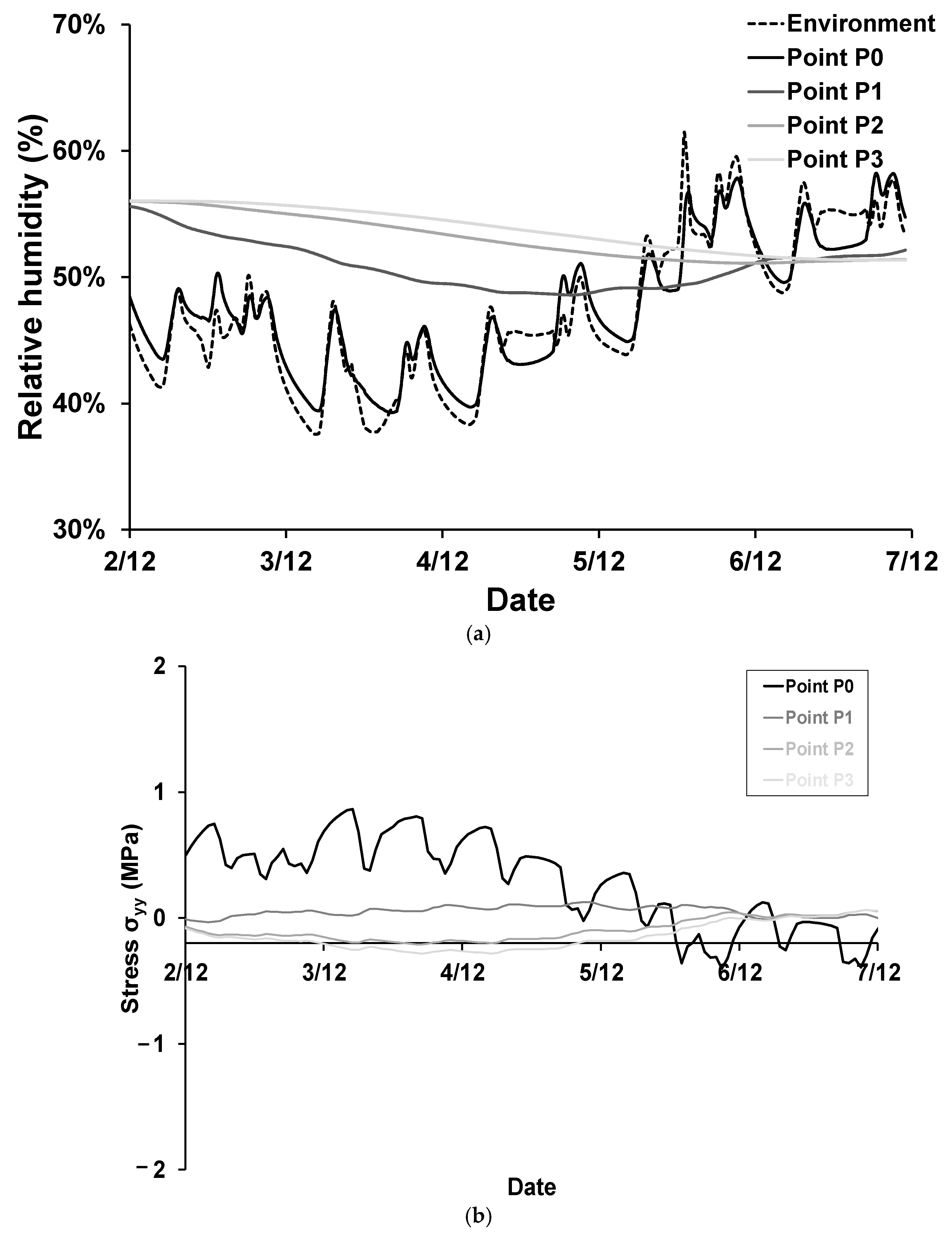
4.1.3. Mechanical Impacts

A mechanical calculation was carried out every hour over the course of a full simulation year. The mechanical boundary conditions applied to the wall were as follows (Figure 20):

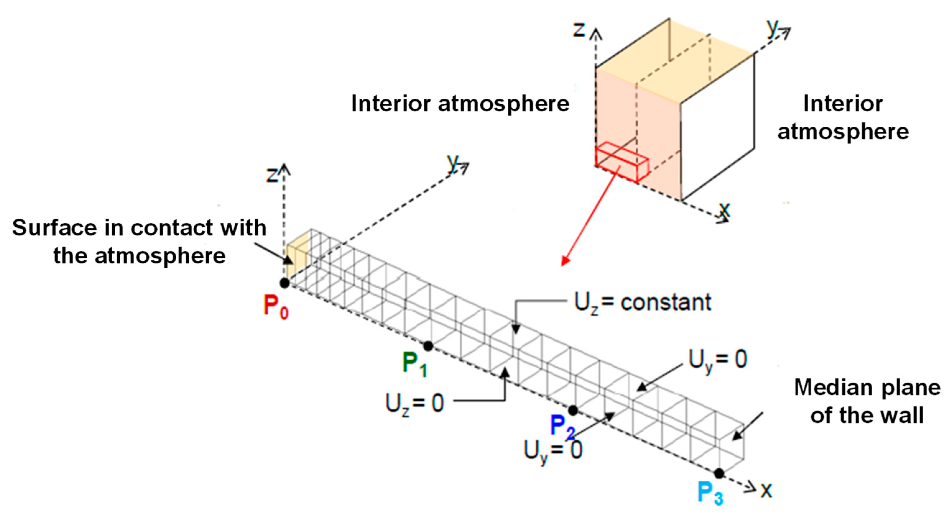
• Imposition of horizontal displacements Uy parallel to the plane of the wall at an identical but free value.
• Imposition of vertical displacements Uz at an identical but free value.

The reference water content chosen for the calculation of eigenstrain due to shrinkage or swelling corresponds to the equilibrium water content under average annual ambient relative humidity. The stresses are calculated using a modulus of elasticity that depends on both the water content and the sign (compression or tension) of the stress σ_yy.

Figure 21 shows the annual evolution of stresses calculated under different climatic scenarios at different wall depths. The positions of the calculation points are shown in Figure 20. According to the results of these simulations, the maximum stresses obtained in tension or compression are those recorded near the wall surface (point P₀). The stresses calculated at points P₁, P₂, and P₃ are lower and therefore less sensitive to shrinkage and swelling. This outcome should be viewed in relation to the thickness of the “active layer," which ensures moisture exchange under transient conditions. It can also be observed that the critical tensile strength values are reached in the cold period (0.86 MPa) during the first week of December (3 December); this day corresponds to the annual minimum in indoor relative humidity. Furthermore, the minimum component of σ_yy = 0.93 MPa is obtained during the summer period (1 June).

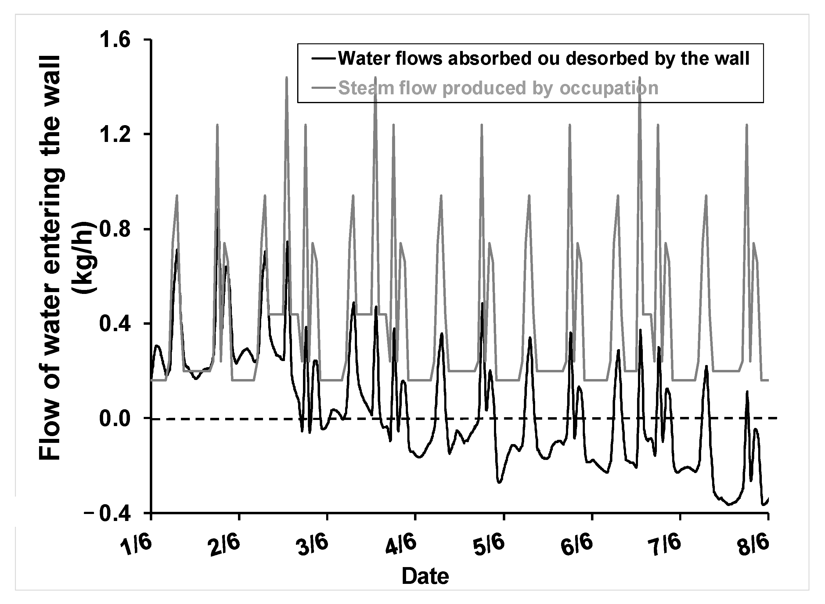
4.2. A Detailed Study of a Critical Week

Figure 22a shows the evolution of relative humidity during the period of lowest relative humidity and the corresponding stress due to water-induced shrinkage/expansion at different wall depths (Figure 22b).

The results of this simulation reveal that the water transfer mechanisms are much more intense in the first layer of the wall (point P₀) and then become progressively more uniform through the thickness of the wall. It should also be noted that the humidity calculated at the level of the active layer conforms to the ambient equilibrium of the room, with a certain phase shift due to surface resistance. This dynamic change between the wall and the external environment exposes the first layer of the wall to critical situations (absorption and restitution of moisture), leading to expansion or shrinkage in the wall and generating stresses σ_yy up to 0.86 MPa in tension and −0.28 MPa in compression (Figure 22b).

The tensile stresses obtained lie above the experimentally determined threshold value. It could therefore be imagined that the wall would crack under the thermohydric cycles, yet the observations suggest otherwise.

i.

This is one-dimensional behavior, which does not take into account the effects of possible confinement due to the weight of the wall and the stress caused by the expansion of the wall elements on the sides (y direction).

ii.

There is a wide dispersion in the experimental results. Also, from a design perspective, while it is sensible to take a characteristic or average value, in the aim of modeling actual wall behavior, a probabilistic approach should be used due to the heterogeneity, which leads to great variability in the physical and mechanical characteristics.

iii.

Microcracks could form, though they would ultimately close under the effect of confinement and humidity; they should still be taken into account through damageable behavior.

5. Conclusions

This work presents a numerical study of the thermo-hygro-mechanical behavior of two types of walls (rammed earth/plaster) when in service. The simulated dwelling is a T4 detached house. The scenario for occupancy and use of the dwelling was defined in the RT2012 rules of Th-BCE. To feed the numerical model, we developed a multidisciplinary experimental campaign to characterize the thermal, hydric, and mechanical properties under different humidity conditions. The simulation did provide two key results:

• A 50% reduction in annual humidity amplitude occurs with an earth wall compared to a classical plaster wall;
• The stress variation is maximized at the wall surface, which could lead to crack formation;
• Lastly, from a more general perspective, the conclusions drawn from this work may lead to numerous prospects for future studies, namely:
• Improvement of the numerical model by taking free water transfer into account in order to extend the results obtained in the hygroscopic domain to the capillary domain, in addition to modeling the drying phase during the wall construction phase;
• Characterization of the mechanical behavior of earth bricks in the capillary domain in order to control the wall construction phase;
• Choice of a viscoelastic, or even viscoelastoplastic, approach, which proves to be necessary when incorporating changes in the material submitted to high water content.

References

1. ADEME. Agence de l’Environnement et de la Maitrise de l’Energie. 2015. Available online: https://www.ademe.fr (accessed on 12 October 2023).
2. Colin, S.; Fendrich, Y.; Lefranc, S.; Mathieu, B.; Morel, R.; Nouvellon, Q.; Polard, G.; Rateau, G. Chiffres Clés du Logement; Ministry of Ecological Transition: Paris, France, 2022.
3. Jaquin, P.; Augarde, C.; Toll, D.G.; Gallipoli, D. The strength of unstabilised rammed earth materials. Géotechnique 2009, 59, 487–490. [Google Scholar] [CrossRef]
4. Kherrouf, S.; Covalet, D. Mieux Comprendre les Transferts de Masse Pour Maitriser les Transferts de Chaleur; EDF R&D Département EnerBAT: Paris, France, 2010. [Google Scholar]
5. Courgey, S.; Oliva, J.-P. La Conception Bioclimatique; Editions Terre Vivante: Rhone-Alpes, France, 2006; ISBN 9782914717212. [Google Scholar]
6. Pittet, D.; Kotak, T.; Jagadish, K.S.; Kotak, T.; Vaghela, K.; Zaveri, P.; Sareshwala, H.; Gohel, J. Environmental impact of building technologies, a comparative study in Kutch District, Gujarat State, India. In Technologies and Innovations for Development; Springer: Paris, France, 2012. [Google Scholar] [CrossRef]
7. Cagnon, H.; Aubert, J.E.; Coutand, M.; Magniont, C. Hygrothermal properties of earth bricks. Energy Build. 2014, 80, 208–217. [Google Scholar] [CrossRef]
8. Maillard, P.; Aubert, J.E. Effects of the anisotropy of extrudes earth bricks on their hygrothermal properties. Constr. Build. Mater. 2014, 63, 56–61. [Google Scholar] [CrossRef]
9. Minke, G. Building with Earth: Design and Technology of a Sustainable Architecture; Birkhauser: Basel, Switzerland, 2006. [Google Scholar]
10. Allinson, D.; Hall, M. Hygrothermal analysis of a stabilished rammed earth test building in the UK. Energy Build 2010, 42, 845–852. [Google Scholar] [CrossRef]
11. Guettala, A.; Abibsi, A.; Houari, H. Durability study of stabilized earth concrete under both laboratory and climatic conditions exposure. Constr. Build. Mater. 2006, 20, 119–127. [Google Scholar] [CrossRef]
12. McGregor, F.; Heath, A.; Shea, A.; Lawrence, M. The moisture buffering capacity of unfired clay mansonry. Build. Environ. 2014, 82, 599–607. [Google Scholar] [CrossRef]
13. Jeannet, J.; Pollet, G. La Thermique du Pisé: Modernité de la Construction en Terre; Actes de Colloque: Paris, France, 1986; ISSN 0246-5612. [Google Scholar]
14. Taylor, P.; Luther, M.B. Evaluating rammed earth walls: A case study. Solar Energy 2004, 76, 79–84. [Google Scholar] [CrossRef]
15. Soudani, L.; Woloszyn, M.; Fabbri, A.; Morel, J.-C.; Grillet, A.-C. Energy evaluation of rammed earth walls using long term in-situ measurements. Solar Energy 2017, 141, 60–70. [Google Scholar] [CrossRef]
16. Khoshbakht, M.; Lin, M.-W. A finite element model for hygro-thermo-mechanical analysis of masonry walls with FRP reinforcement. Finite Elem. Analy Des. 2010, 46, 783–791. [Google Scholar] [CrossRef]
17. Steeman, H.-J.; Van Belleghem, M.; Janssens, A.; De Paepe, M. Coupled simulation of heat and moisture transport in air and porous materials for the assessment of moisture related damage. Build. Environ. 2009, 44, 2176–2184. [Google Scholar] [CrossRef]
18. Zonno, G.; Aguilar, R.; Boroschek, R.; Lourenço, P.B. Analysis of the long and short-term effects of temperature and humidity on the structural properties of adobe buildings using continuous monitoring. Eng. Struct. 2019, 196, 109299. [Google Scholar] [CrossRef]
19. Zonno, G.; Aguilar, R.; Boroschek, R.; Lourenço, P. Experimental analysis of the thermohygrometric effects on the dynamic behavior of adobe systems. Constr. Build. Mater 2019, 208, 158–174. [Google Scholar] [CrossRef]
20. Laou, L. Evaluation du Comportement Mécanique sous Sollicitations Thermo-Hydriques d’un mur Multimatériaux (Bois, Terre crue, Liants Minéraux) Lors de sa Construction et de son Utilisation. Ph.D. Thesis, University of Limoges France, Limoges, France, 2017. Available online: https://www.theses.fr/2017LIM00066≠ (accessed on 12 October 2023).
21. Laou, L.; Aubert, J.-E.; Yotte, S.; Maillard, P.; Ulmet, L. Hygroscopic and mechanical behaviour of earth bricks. Mater. Struct. 2021, 54, 116. [Google Scholar] [CrossRef]
22. TH-b-CE, 2012, Fascicule TH-u Matériaux, Arrêté du 18 May 2011. Available online: https://rt-re-batiment.developpement-durable.gouv.fr/IMG/pdf/thu-ex_5_fascicules.pdf (accessed on 12 October 2023).
23. Samson, E.; Marchand, J.; Beaudoin, J. Describing ion diffusion mechanisms in cement based materials using the homogenization technique. Cem. Concr. Res. 1999, 29, 1341–1345. [Google Scholar] [CrossRef]
24. Lemaire, T.; Moyne, C.; Stemmelen, D. Modelling of electro-osmosis in clayey materials including pH effects. Phys. Chem. Earth 2007, 32, 441–452. [Google Scholar] [CrossRef]
25. Bourbatache, K. Modélisation du Transfert des Ions Chlorures dans les Matériaux Cimentaires par Homogénéisation Périodique. Ph.D. Thesis, University of La Rochelle, La Rochelle, France, 2009. [Google Scholar]
26. Moyne, C.; Murad, M. A two-scale model for coupled electro-chemo-mechanical phenomena and onsager’ s reciprocity relations in expansive clays: I homogenization analysis. Trans. Porous Media. 2006, 62, 333–380. [Google Scholar] [CrossRef]
27. Luikov, A. Heat and Mass Transfer in Capillary Porous Bodies. Adv. Hea Trans. 1966, 1, 123–184. [Google Scholar] [CrossRef]
28. Daïan, J.F. Processus de Condensation et de Transfert d’eau dans un Matériau Méso et Macroporeux. Etude Expérimentale du Mortier de Ciment. Ph.D. Thesis, University of Grenoble, Grenoble, France, 2012. [Google Scholar]
29. Janssen, H. Simulation efficiency and accuracy of different moisture transfer potentials. Build. Perform. Simul. 2014, 7, 379–389. [Google Scholar] [CrossRef]
30. Medjelekh, D. Caractérisation Multi-Echelle du Comportement Thermo Hydrique des Enveloppes Hygroscopiques. Ph.D Thesis, University of Limoges, Limoges, France, 2015. [Google Scholar]
31. Künzel, H.M.; Kiessl, P. Simultaneous Heat and Moisture Transport in Building Components: One-and Two-Dimensional Calculation Using Simple Parameters; Fraunhofer Institue of Building Physics: Stuttgart, Germany, 1995. [Google Scholar]
32. Pedersen, C. Prediction of moisture transfer in building constructions. Build. Environ. 1992, 27, 387–397. [Google Scholar] [CrossRef]
33. Philip, J.; De Vries, D. Moisture movement in porous material under temperature gradients. Trans. Am. Geophys. Union 1957, 38, 222–232. [Google Scholar] [CrossRef]
34. Qin, M.; Belarbi, R.; Aït-Mokhtar, A.; Nilsson, L. Coupled heat and moisture transfer in multi-layer building materials. Constr. Build. Mater. 2009, 23, 967–975. [Google Scholar] [CrossRef]
35. Qin, M.; Belarbi, R.; Aït-Mokhtar, A.; Seigneurin, A. An analytical method to calculate the coupled heat and moisture transfer in building materials. Int. Commun. Heat Mass Transf. 2006, 331, 39–48. [Google Scholar] [CrossRef]
36. Davie, C.; Pearce, C.; Bicanic, N. A fully generalised, coupled, multi-phase, hygrothermo-mechanical model for concrete. Mater. Struct. 2010, 43, 13–33. [Google Scholar] [CrossRef]
37. Thibeault, F.; Marceau, D.; Younsi, R.; Kocaefe, D. Numerical and experimental validation of thermo-hygro-mechanical behaviour of wood during drying process. Int. Commun. Heat Mass Transf. 2010, 37, 756–760. [Google Scholar] [CrossRef]
38. Nguyen, V.-T.; Jiabin, L.; Ferhun, C.-C. Microplane constitutive model m4lfor concrete. I: Theory. Comput. Struct. 2013, 128, 219–229. [Google Scholar] [CrossRef]
39. Gonzalez, I.J.; Scherer, G. Effect of swelling inhibitors on the swelling and stress relaxation of clay bearing stones. Environ. Geol. 2004, 46, 364–377. [Google Scholar] [CrossRef]
40. Cast3M. Finite Element Software, Commissariat Français à l’Energie Atomique (CEA). 2017. Available online: https://www.cast3M.cea.fr (accessed on 12 October 2023).
41. ISO 12571:2021; Performance Hygrothermique des Matériaux et Produits pour le Bâtiment—Détermination des Propriétés de Sorption Hygroscopique. ISO Standards: Geneva, Switzerland, 2000.
42. ISO 12570:2000; Performance Hygrothermique des Matériaux et Produits pour le Bâtiment—Détermination du Taux d’Humidité par Séchage à Chaud. ISO Standards: Geneva, Switzerland, 2013.
43. Merakeb, S. Modélisation des Structure en Bois en Environnement Variable. Ph.D. Thesis, University of Limoges, Limoges, France, 2006. [Google Scholar]
44. Nguyen, T.-A. Approches Expérimentales et Numériques pour l’Etude des Transferts Hygroscopiques Dans le Bois. Ph.D. Thesis, Université de Limoges, Limoges, France, 2014. [Google Scholar]
45. Droin-Josserand, A.; Taverdet, J.L.; Vergnaud, J.M. Modelling the absorption and desorption of moisture by wood in an atmosphere of constant and programmed relative humidity. J. Wood Sci. Technol. 1988, 22, 299–310. [Google Scholar] [CrossRef]
46. ISO 12572:2016; Performance Hygrothermique des Matériaux et Produits pour le Bâtiment—Détermination des Propriétés de Transmission de la Vapeur d’eau. ISO Standards: Geneva, Switzerland, 2000.
47. Collet, F. Caractérisation Hydrique et Thermique de Matériaux de Génie Civil à Faibles Impacts Environnementaux. Ph.D. Thesis, University of Rennes, Rennes, France, 2004. [Google Scholar]
48. Hall, M.; Allinson, D. Assessing the effects of soil grading on the moisture content-dependent thermal conductivity of stabilised rammed earth materials. Appl. Therm. Eng. 2009, 29, 740–747. [Google Scholar] [CrossRef]
49. CTMNC. Centre Technique de Matériaux Naturels de Construction (CTMNC), Service Céramique R&D, 11 Avenue d’Ariane, 87068, Limoges Cedex, France. Available online: https://cmtnc.polaris-creations.fr (accessed on 12 October 2023).
50. Fontaine, L. Cohésion et Comportement Mécanique de la Terre Comme Matériau de Construction. Ph.D. Thesis, University of Limoges, Limoges, France, 2004. Available online: https://dumas.ccsd.cnrs.fr/dumas-03230968 (accessed on 12 October 2023).
51. Aubert, J.; Maillard, P.; Morel, J.C.; Al Rafii, M. Towards a simple compressive strength test for earth bricks? J. Mater. Struct. 2016, 49, 1641–1654. [Google Scholar] [CrossRef]
52. Pkla, A.; Mesbah, A.; Rigassi, V.; Morel, J. Comparaison de méthodes d’essais de mesures des caractéristiques mécaniques des mortiers de terre. Mater. Struct. 2003, 36, 108–117. [Google Scholar] [CrossRef]
53. NF P94-422; Roches—Détermination de la Résistance à la Traction—Méthode Indirecte—Essai Brésilien. AFNOR: Paris, France, 2001.
54. Heath, A.; Walker, P.; Fourie, C.; Lawrence, M. Compressive strength of extruded unfired clay masonry units. J. Constr. Mater. 2009, 162, 105–112. [Google Scholar] [CrossRef]
55. Pirat, P.E.; Filloux, R. Etude de l’effet d’échelle sur le matériau terre. In Projet d’Initiation à la Recherche et au Développement; INSA: Lyon, France, 2012. [Google Scholar]
56. Jacquin, P.-A.; Augarde, C. Earth Building—History, Science and Conservation; IHS BRE Press: Bracknell, UK, 2012; ISBN 978-1-84806-192-7. [Google Scholar]
57. Hakimi, A.; Yamani, N.; Ouissi, H. Résultats d’essais de résistance mécanique sur échantillon de terre comprimé. J. Mater. Struct. 1996, 29, 600–608. [Google Scholar] [CrossRef]
58. Givoni, B. L’Homme, le Climat et l’Architecture; Editions du Moniteur: Paris, France, 1978. [Google Scholar]
59. Kwiatkowski, L.; Woloszyn, M.; Roux, J.-J. Influence of sorption isotherms hysteresis effect on indoor climate and energy demand for heating. J. Appl. Therm. Engine 2011, 31, 1050–1057. [Google Scholar] [CrossRef]
Figure 1. Dwelling layout and placement of the earth brick walls.
Buildings 13 03061 g001
Figure 2. Diagram explaining the approach and boundary conditions used to simulate the behavior of the two partition walls.
Buildings 13 03061 g002
Figure 3. Scenario adopted for steam production.
Buildings 13 03061 g003
Figure 4. Algorithm for coupling mass and heat transfer, along with the mechanical calculation.
Buildings 13 03061 g004
Figure 5. Comparison of experimental vs. numerical results for the sorption-desorption curve.
Buildings 13 03061 g005
Figure 6. Geometric model used to simulate apparent permeability: meshed by FE, and example of water and heat fields calculated during the adsorption phase (75% to 90% RH, time: 12 h).
Buildings 13 03061 g006
Figure 7. Numerical values for apparent permeability vs. water content.
Buildings 13 03061 g007
Figure 8. Thermal conductivity vs. water content.
Buildings 13 03061 g008
Figure 9. Experimental device for measuring dimensional variations, as developed by the CTMNC.
Buildings 13 03061 g009
Figure 10. Evolution of eigenstrain vs. (a) time and (b) water content.
Buildings 13 03061 g010
Figure 11. (a) depiction of the failure mode of the Brazilian test; and (b) layout of strain gauges on the specimen.
Buildings 13 03061 g011
Figure 12. Compressive and tensile strength vs. water content.
Buildings 13 03061 g012
Figure 13. Modulus of elasticity vs. water content.
Buildings 13 03061 g013
Figure 14. Annual changes in indoor relative humidity for two partition walls.
Buildings 13 03061 g014
Figure 15. Change in indoor relative humidity compared with outdoor humidity during a sequence of (a) winter and (b) summer.
Buildings 13 03061 g015
Figure 16. Givoni diagram for: (a) basic partition walls; and (b) earth partition walls.
Buildings 13 03061 g016
Figure 17. Water flows are exchanged by the brick wall, and the resulting steam flow is produced.
Buildings 13 03061 g017
Figure 18. Changes in indoor relative humidity during (a) winter and (b) summer, using self-regulating and humidity-controlled ventilation.
Buildings 13 03061 g018
Figure 19. Ventilation rates for the two types of CMV and the different types of partition walls.
Buildings 13 03061 g019
Figure 20. Mechanical model for the homogeneous wall and boundary conditions.
Buildings 13 03061 g020
Figure 21. Annual evolution of stresses at different wall depths.
Buildings 13 03061 g021
Figure 22. (a) Changes in external and internal relative humidity at different points in the wall, and (b) Changes in stresses generated by shrinkage and swelling.
Buildings 13 03061 g022