1. Introduction
Conservation of the built heritage through regular maintenance is the simplest, most economical and effective way to preserve it. Building maintenance, which is included in Facility Management (FM) activity, represents a sustainable practice, since it reduces environmental impact by reducing the consumption of resources and emission of pollutants, and promotes economic development by creating jobs and encouraging economic activity [
1]. The identification of building anomalies and the prediction of the degradation of a building to extend its service life are important tasks to reach an efficient FM. However, the interpretation and prediction of the degradation state of a building requires specialized human professionals and several building inspections, which are time-consuming and require long-distance travel, which can be supported with New Technologies and programming algorithms [
2]. Several building anomalies have common features, patterns, contours, and shapes which Artificial Intelligence (AI) and regression algorithms can handle. The extent to which computer vision algorithms employing AI and Deep Learning (DL), the records of defects and targets that anticipate building anomalies, can be relevant in helping to predict failures and adjust future interventions. Some institutional buildings, like health buildings, must keep their performance at the highest level due to equipment and systems and the use of the building. On the other hand, other types of buildings are just required to maintain a failure-free performance to minimize the costs of maintenance tasks [
3].
This work intends to discuss the application of methodologies utilizing AI algorithms and Python programming to improve the automatized identification of building anomalies and to achieve future prediction of building degradation. For this purpose, the goals were: (1) the automatization of the recognition and classification of building anomalies, connected with a Building Information Modelling (BIM) model; (2) obtaining degradation curves based on different degradation functions; and (3) prediction of building degradation based upon the regression of previous conservation state surveys. The first part of the work was dedicated to the classification algorithm, which provides automatized recognition of building anomalies. Then, a comparison of the results with other research was performed. Afterwards, the development of a regression model to predict future building degradation was created. So, a DL model with computer vision algorithms based on the Pytorch Library has been developed on the past and current records of buildings’ conditions and the Building Condition Assessment (BCA) method supported by Key Performance Indicators (KPIs). Computer vision techniques, namely Convolutional Neural Networks (CNN), were used for image recognition, which permits fast defect identification. Besides that, multi-label classification and several Machine Learning (ML) architectures were also used. This model will be able to predict future degradation and the optimum moment at which components must be intervened or replaced, and it will be available to all stakeholders because the BIM environment acts as a repository for information that can be processed and extracted.
2. Overview
In recent years, the use of AI for image classification has been implemented and tested. AI has been used as a means of assisting health diagnosis, and Deep Learning techniques have been developed to identify diverse pathologies such as lung nodules or Alzheimer’s [
4,
5]. In the Architecture, Engineering, Construction and Operation sector (AECO), namely in the field of Facility Management (FM), image classification algorithms for the detection of building anomalies have been studied but still need to be improved. In this field, Grilli et al. (2019) [
6] developed different supervised learning approaches based on DL algorithms to classify architecture components on 3D point clouds in an automatized way. Based on sophisticated image processing, studies have been developed by Mohan and Poobal (2018) [
7] and Ribeiro et al. (2020) [
8] for the automatic diagnosis of several types of reinforced concrete (RC) defects, including biological colonies, efflorescence, fissures, and exposed steel rebars. Also, Shin et al. (2020) [
9] developed a CNN algorithm able to recognize concrete damage in an automated way with 98.9% accuracy. Convolutional Neural Networks (CNNs) and computer vision techniques were used by Rodrigues et al. (2022) [
2] to automate the detection and classification of flaws in historic structures. An algorithm was utilized by Bretti and Ceseri (2022) [
10] to forecast how climate change will affect the progression of carbonation-related Portland cement degradation.
Haznedar et al. (2023) [
11] also used Artificial Intelligence based on Deep Learning methods to complete deteriorated and deformed scans allowing the assembly of point clouds.
Automatic anomaly detection is important and useful to detect the anomaly in an easy way which should be supported by a well-known degradation mechanism. The current context of economic depression, ecological saturation, and excess of degraded buildings requires a more careful FM approach. The challenges for the AECO sector include the implementation of preventive conservation and maintenance habits and practices, moving from a reactive to a preventive philosophy. The degradation of buildings depends on several factors that have been analyzed by researchers to develop measures that mitigate degradation mechanisms and extend their service life [
12]. More than ever, nowadays, due to the climate changes and global warming that planet Earth is experiencing, elements with severe signs of degradation may have a longer service period than those with fewer signs of deterioration [
12,
13,
14]. So, FM policies require a more careful understanding of degradation mechanisms based on real data to adapt each curve to each case study [
1].
Artificial Intelligence algorithms need big datasets to provide a good and credible result for predictions. Whenever the dataset is small for future prediction purposes, like predicting future building degradation, regression is the best option to obtain more accurate predictions according to the past data.
Thomas et al. (2016) [
15] stated that there is an absence of studies analyzing the deterioration patterns of building materials. The authors also referred to linear, exponential, and polynomial curves that can represent the degradation patterns of most materials.
The degradation curve types can represent different patterns of evolution of the degradation and degradation paces [
16]. Four patterns of deterioration paths are defined by these authors, who studied deterioration patterns of building and system components based on their condition monitored in situ. A linear degradation curve represents a loss in component performance of cladding due to a continuous and consistent deterioration agent.
A convex degradation curve means a physical failure of the entire system of exterior cladding due to physical or chemical phenomena. A concave degradation curve is typical of anomalies caused by microorganisms or cyanobacteria development on claddings. The curve starts with a fast loss in performance, and then the decay slows down over time. An S-shape degradation curve represents a deterioration mechanism that changes its intensity over time. This type of decay usually arises in the early ages of systems.
Based on the knowledge of the aforementioned authors, the degradation functions of materials were explored in the literature. Degradation curves are based on deterministic models, and they represent materials’ performance and can be applied to each building defect considering several associated degradation factor combinations [
17]. Degradation curves can be obtained with the adjustment of degradation functions, which represents the degradation verified in test samples over time. The morphology of the curves should adequately fit the general progress of the points (data field) on a degradation graph [
18]. At the beginning of the work, several degradation curves were explored for each constructive system, namely for windows [
19], concrete surfaces (Serralheiro, 2016) [
20], and roofs [
21]. Moreover, functions representing a loss in performance over time which take several degradation factors into account were also found, such as Gompertz curves [
17,
22], Potential curves (Garrido et al., 2012b) [
22], and Weilbul curves (Garrido et al., 2012b) [
22]. The Weibull distribution was presented in the US in 1951 by Walodi Weibull, based on his research on material fatigue. It is a versatile method used to represent the lifespan of a building until its failure due to degradation phenomenon, and it has a remarkable ability to fit a wide variety of possible shapes of real probability distributions. Regarding Gompertz curves [
17,
22], asymptotes at the early and final ages, which correspond to the initial years with no defect and the final years with the highest defect level, are what define these types of curves. The degradation rate of the model lies between these two extremes. Garrido (2010) [
18], Costa (2011) [
23], and Paulo et al. (2014) [
17] compared adjustments of the data for the degradation curves of Gompertz, Weibull, and Potential. According to their results, Gompertz curves are the ones able to provide a better adjustment to reality and a more consistent result. Potential curves present, similarly to Gompertz curves, an initial plateau that reflects a period of initiation of degradation, followed by a gradual increase in the degradation rate. However, unlike Gompertz curves, Potential curves do not present a plateau at the end of the curve, and the degradation rate continuously increases until the maximum value of the anomaly extension is reached.
So, in this study, the concept proposed by Shohet et al. (1999) [
16], Shohet et al. (2002) [
3], and used by Thomas et al. (2016) [
15] is adopted. For the definition of degradation curves, building performance is assumed to deteriorate from the highest condition level (whenever the materials are installed), with a decrease in their performance until the end of service life for each material. This study aims to perform automatic anomaly detection using ML and DL and based on building surveys recorded over the years.
Besides that, this study intends to present the degradation process using degradation functions, the data field collected, and regression algorithms. Degradation functions include loss in performance as the dependent variable and time as the independent variable. For this purpose, the qualitative data from several technical visits to the building were converted to quantitative numerical data. Then, with a regression analysis, several degradation functions were tested, and the parameters which better fitted the functions to the data field collected from the case study were found. The tested degradation functions were the Gompertz, Weibull, Potential, two-degree, and third-degree polynomial functions [
13]. The degradation curves will be updated as long as new technical visits to the building are carried out and new evaluations are received.
3. Methodology
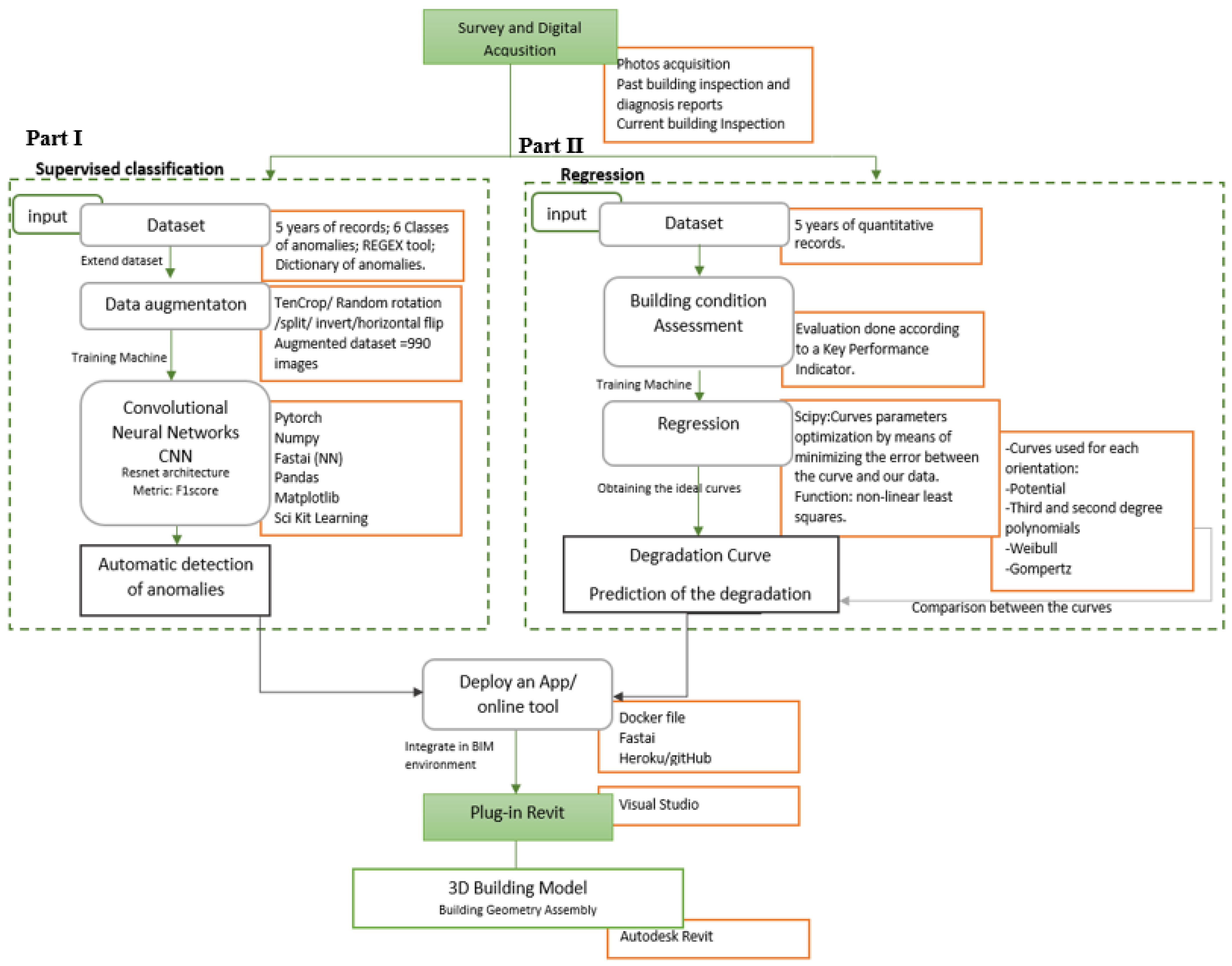
Figure 1 presents the methodology and the proposed tasks to accomplish the main objectives, which are: to provide tools for automatic anomaly detection (Part I) and predict future building degradation (Part II).
Automatic anomaly detection is the first part of this work, achieved through the use of supervised classification. The model was trained using a dataset collected over 5 years. However, computer vision algorithms require large datasets to be effective. So, the expansion of the number of images in the dataset was possible with data augmentation techniques. Then, the model was trained for the automatic detection of anomalies through Convolutional Neural Networks (CNN) in Python programming language. For this purpose, Pytorch 2.1.0+cu118, Numpy 1.23.5, Fastai 2.7.13, Matplotlib 3.7.1, and Sci Kit Learning 1.2.2 were the libraries used. Different layers of Resnet architecture were used to train the model, and the metric F1 score was implemented to indicate the overall quality of the model. In the end, this model based on CNNs will be able to accept images and provide automatic analysis of those images. Afterwards, this tool will be deployed as an app which can be associated with Autodesk Revit 2022 software as a plug-in.
The second part of the work consists of predicting building degradation. Similarly to the first part of the work, a dataset of images of building anomalies, as well as their quantified state of conservation using Key Performance Indicators (KPI), collected over 5 years, was used in this study. This part of the work consists of a multi-series regression based on a dataset of previous evaluations of the building degradation state carried out with a Key Performance Indicator (KPI). The multi-series regression tested several functions of the several degradation mechanisms, which were adjusted to the data recorded. This makes it possible to obtain a prediction of the future likely moment that will require intervention based on the previous defects of the building. The next chapter will describe the implementation of the methodology, as employed in a case study. It would be also an added value for this tool to be associated with a 3D model through the use of an app as a Plug-in in Autodesk Revit, which would be possible using Visual Studio 2019.
4. Case Study
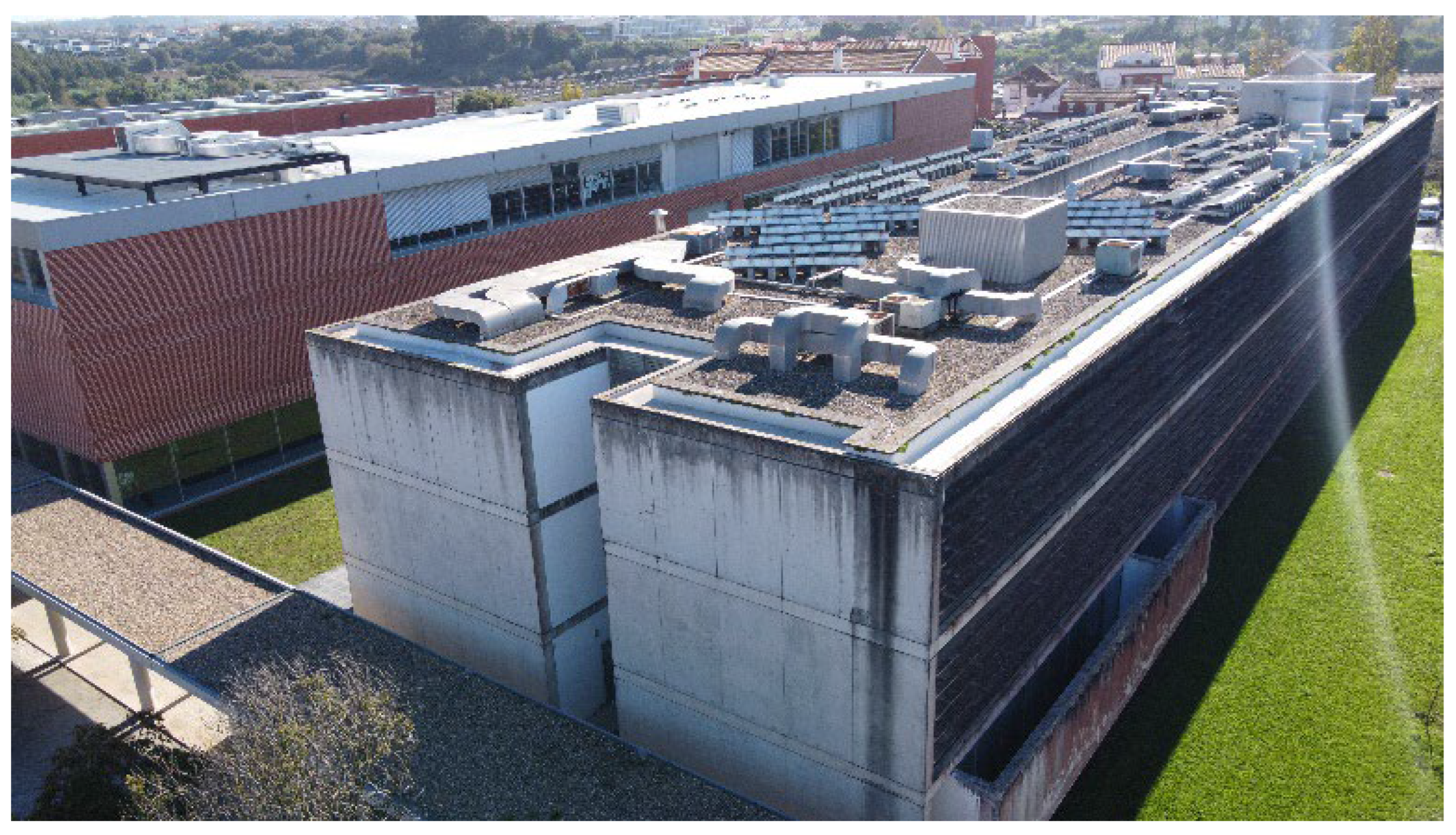
This methodology was developed and applied to a building on the campus of the Department of Geosciences, University of Aveiro, Aveiro, Portugal. The building was designed by architect Souto Moura and was constructed in 1993. The building has four floors. The basement is a warehouse. The first and second floors consist of classrooms and laboratories. The staff offices are on the 3rd floor. The northeast and southwest façades consist of concrete structures. The northwest and southeast façades consist of exposed concrete walls that support glazed openings in all extensions of these façades. These façades consist of a pink marble shading system supported by a steel structure attached to a concrete structure. This department has a rectangular shape with two entrances on the northeast and southwest façades.
Figure 2 shows the surveyed building.
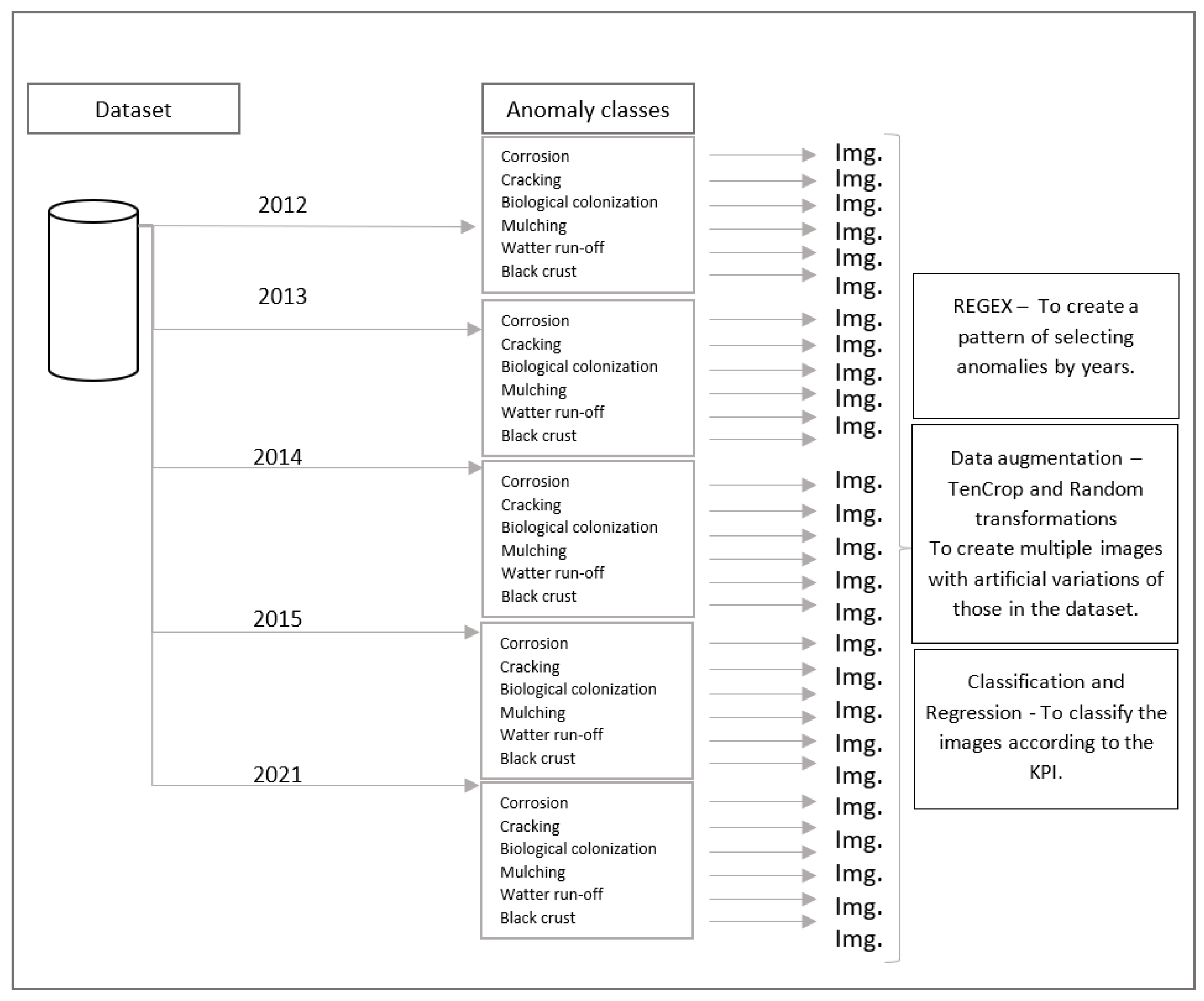
The first task of the methodology consisted of data acquisition, for which several past reports of building anomalies and the evolution of the anomalies over the years (2012, 2013, 2014, 2015, and 2021) were evaluated and recorded. A building inspection was also conducted to complete the dataset with current and updated information. A dataset was then compiled from images of anomalies within the case study building. These images were organized and classified by year and type of anomaly (
Figure 3) (a dictionary of images was developed using a DL one-hot coding process). Those images were used as input parameters for developing the image recognition process in the DL model.
The anomalies in
Figure 3 were selected because they were identified in the case study, and they were subject to records from their state of conservation over 5 years, allowing analysis of their evolution.
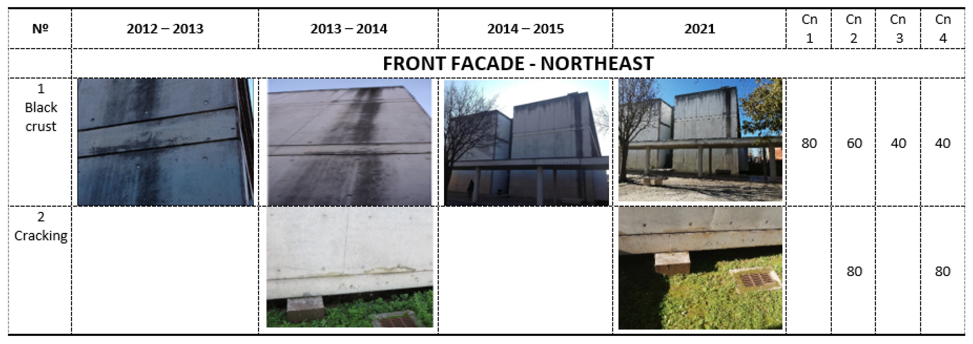
Besides that, each building anomaly and each photograph was classified and quantified according to a KPI first developed by Shohet et al. (2003) [
24] and optimized by [
25] (
Figure 4), in which Cn is the measure for the current condition of the system.
After, data processing took place. Supervised classification consists of the automatic identification and classification of building defects based on computer vision algorithms, as well as the automatic prediction of the degradation of the components based on the historic data inputted.
The process consists of two phases: (i) the automatic identification of defects of the building envelope based on collected images; (ii) the prediction of the building degradation of the failure mode studied.
4.1. Automatization of the Recognition of the Building Anomalies
DL tools were used to achieve the automatic identification of the registered pathologies based on the gathered pictures and the use of image processing technologies. This step deals with supervised classification where a DL model was trained considering representative data classified by users. The model used a computer programming system to process all collected data and automate it in the BIM environment. The DL model data processing and training pipeline was built using the Python programming language and PyTorch [
26] computer vision framework. The model was trained on a single NVIDIA Tesla V100 GPU, and metrics and resulting statistics were generated using scikit-learn (Pedregosa, F., et al., 2011) [
27]. The DL model was made in Jupyter Lab, where PyTorch, fastai, pandas, sklearn, and matplotlib were some of the libraries used to create, analyze, and evaluate the model.
Automatic segmentation and classification were carried out using the PyTorch pipeline, where the images were pre-processed. All images were labelled according to the year and their defects, in 8 classes (each class corresponds to an anomaly). The dataset was composed of images of the anomalies from reports from 2012, 2013, 2014, 2015, and 2021 for the building case study. Each year comprised a folder composed of a set of folders with the name of the building defects.
The full image dataset consisted of 90 images, which were resized to the dimension of 224 × 224 pixels in order to fit into the GPU memory. To avoid overfitting of models, random transformations were imposed into the training dataset to create an augmented dataset, as follows:
- -
Ten crop technique and storing in which each image was randomly cropped into 10 pieces with a fixed dimension of 224 × 224 pixels;
- -
Random rotation of 35°;
- -
Random invert with a probability of 20%;
- -
Random horizontal flip with a probability of 10%;
- -
Transformation of all images to greyscale format to ensure the models can learn structural defect features present in the images. All images were normalized so their pixel color values were in a range of ∈ R [−1, 1] and converted to the tensor format to be used by the CNN model.
An augmented dataset of 990 images was obtained using the transformations applied to the DL model. The full dataset was arbitrarily divided into 80% as a training dataset and 20% as a validation/test dataset. A bias can be introduced using only one dataset; however, the random nature of the dataset selected intended to reduce this issue.
The architecture used for testing the classification task was the Residual Network (ResNet). ResNets were first proposed by He et al. (2016) [
28] and explored and applied by [
2,
29]. In the analysis, the discriminant power of the ResNet was tested, with an increasing number of layers: ResNet-18, ResNet-34, ResNet-50, and ResNet-101.
ResNet, short for Residual Network, is a widely recognized and highly effective deep learning architecture for various computer vision tasks, particularly image classification. That is why it was chosen for this work. Data augmentation techniques were chosen based on their effectiveness and their compatibility with the specific problem and dataset. The batch size and the learning rate were adjusted according to the time it took to run each simulation.
All models were trained using the Adam optimizer [
30] with a maximum learning rate of 5.25 × 10
−5, and models were trained in batches of 64 images and 21 epochs. As a loss function for the model, the CrossEntropyLoss function was used, which is appropriate to this case due to the multiple classes in the dataset. To evaluate the performance of each CNN model, the F1 score metric was used, since it provides the combination of the model’s precision and recall, and its value indicates the general quality of the model. So, based on these considerations, the Top-1 (maximum F1 score value for the first train of the model) and Top-5 (the average of the maximum F1 scores for the next five trains of the model) values of the F1 scores for each ResNet architecture are displayed in
Table 1.
The analysis of these values makes it possible to understand the behavior of the model and whether there are overfitting phenomena.
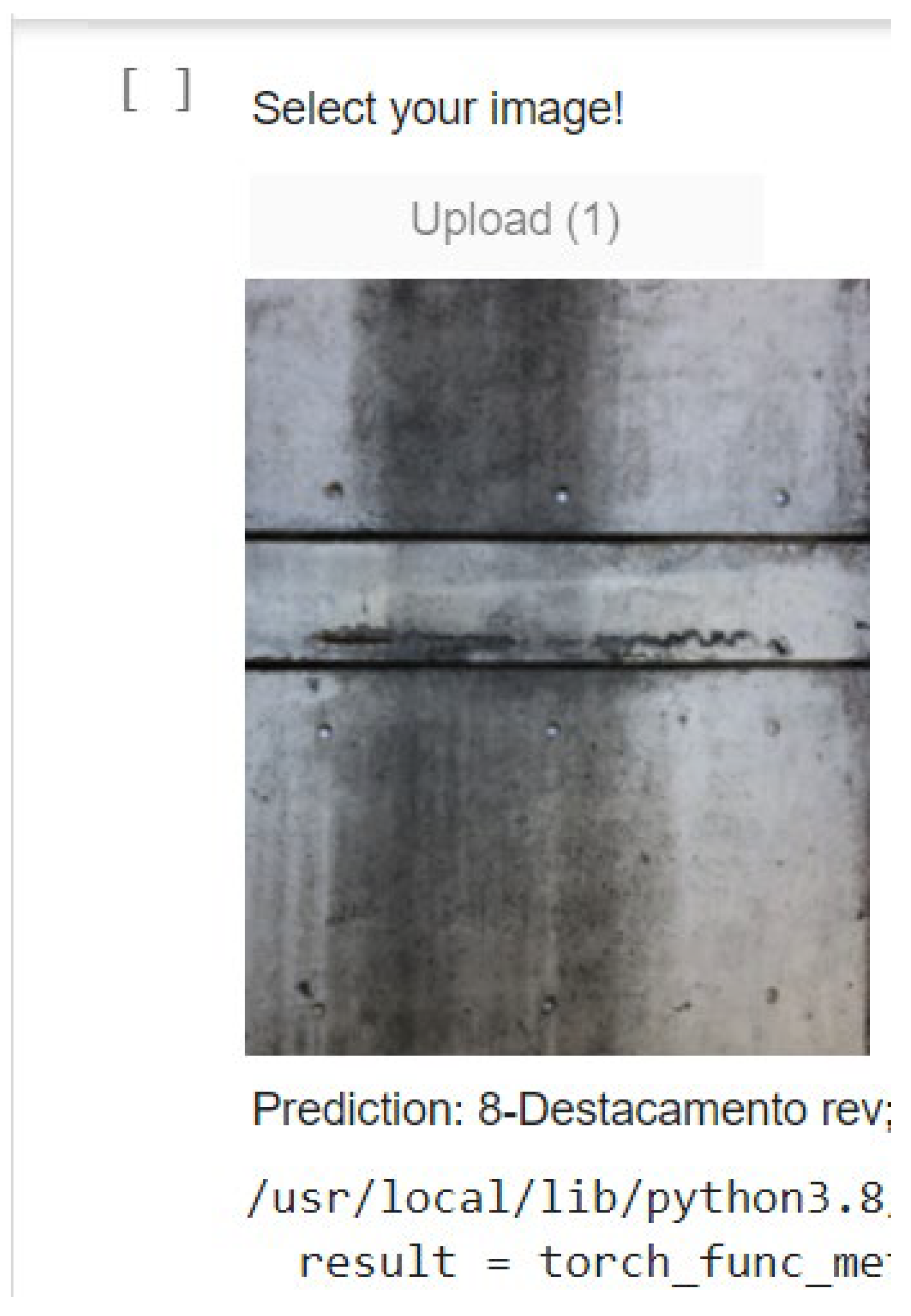
Moreover, the model allows its user to upload a photo which it will then classify according to the type of building anomaly, as presented in
Figure 5.
The metrics and results statistics were obtained using Scikit-learn (Pedregosa, F., et al., 2011) [
27].
The F1 score is a metric that combines precision with recall, and its value indicates the general quality of the model. By means of the architectures used—ResNet—the model achieved more than 70% accuracy. For the architectures used and presented in
Table 1, it is possible to conclude that the precision is above 70% and less than 90%. It is possible to notice that 101- and 18-layer residual nets present a higher quality than 34- and 50-layer residual nets. This can be justified by the size of the original dataset, which can cause the degradation of the model and the accuracy may become saturated (He et al., 2016) [
28]. However, the dataset will continue to increase with photos, which can often improve the model performance, because it is expected to increase the model quality. A low accuracy is also observed for the average of the first five F1 score results for Resnet 34, which is an indicator of overfitting, meaning that layer 34 of Resnet cannot generalize the model well to fit unseen data.
Comparing the results presented in
Table 1 with the results obtained from the work developed by [
2], it is possible to make a comparison from which some improvements can be pointed out.
- -
The classification algorithm helped in obtaining the F1 scores in both cases for the process of image classification.
- -
Comparing the results of both works, the F1 score obtained in the current work demonstrates better classification, since Rodrigues et al. (2022) [
2] obtained an F1 score maximum of just 60.34% for the classification of anomalies of heritage buildings. The reason for this improvement might be due to the data augmentation algorithms used in the models of the current work providing an enlarged dataset of images. The full image dataset of Rodrigues et al. (2022) [
2] consisted of 204 images, and the full image dataset of the current work consists of 990 images, so the current work better avoids the overfitting of the model and consequently provides a higher quality model.
It should be noted that this model will be fed with data in the future, as records of the different types of cracks and other pathologies will be gathered. Afterwards, the model will be able to distinguish the various types of anomalies. For example, now the cracks will be identified with the generic “cracking” classification, which requires an analysis to distinguish each one; in the future, it is anticipated that the model will be able to distinguish the various types of cracks. The Deep Learning model can learn through CNNs. That is why by adding more images, the model can be used as a starting point to detect other types of anomalies. This is why the model can be reproduced for other case studies if it is fed new data.
4.2. Degradation Prediction—Regression Model
The second part of the work aimed to obtain a prediction model which could provide a prediction of degradation and the approximated optimum moment at which to perform future maintenance interventions. For this purpose, regression analysis, which attempts to predict one or more numeric quantities, was implemented. Multiple regression analysis was adopted in this work since, according to Nguyen and A. Cripps. (2001) [
31], it performs better than an artificial neural network for small data sample sizes. The models were trained in an Intel Core i5 1.8 GHz with a graphic board intel HD Graphics 6000 1536 MB with a RAM 8 GB, and several regression curves were found.
The problem definition was characterized by having several numerical calculations of the condition of different building elements for several years. The goal was to forecast the next multiple values of condition for each building element. This part of the work aimed to create degradation curves for each construction system, categorized by their orientation, to establish a threshold for when the condition of the building starts to reach a critical state.
Dataset: for the implementation of this model, a dataset was created. Based on the case study previously presented, and based on the building inspection records, the calculation of each building element condition was possible for several years (1993, 2012, 2013, 2014, 2015, and 2021). The calculation proceeded according to the BCA, employing a KPI. The KPI evaluates the condition of the components, the evolution of degradation, and the frequency of preventive maintenance applied during the components’ service life. The quantitative value of the building condition obtained for each component was organized in an Excel file, according to the year (since 1993, when the building was built, and each year the building was submitted to an inspection) and the building element. The Excel file was imported to the pipeline as a Python data frame structure.
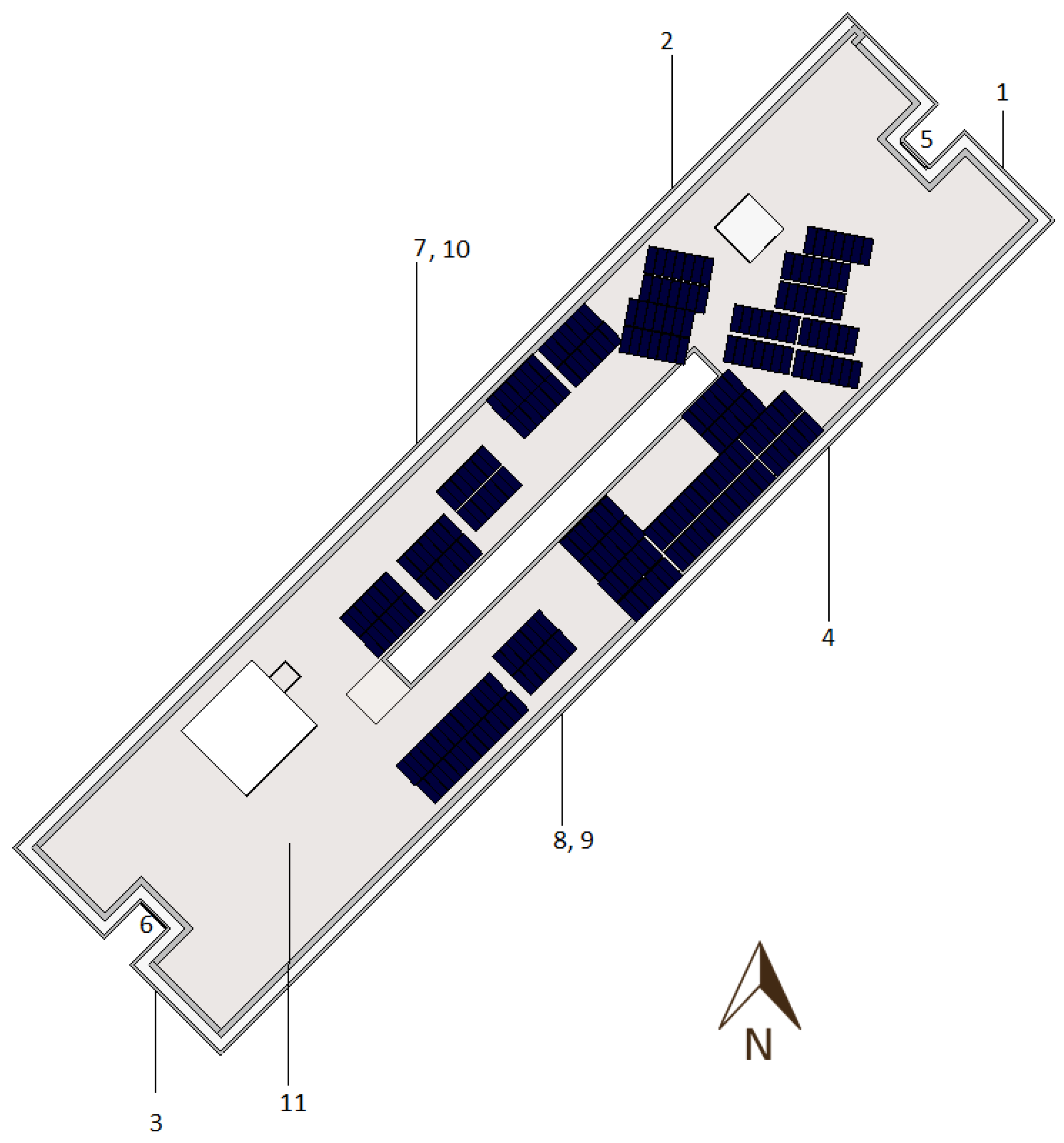
Processing: the pre-processing phase included preparing a multi-step output by receiving multiple parallel time series. It was intended to perform forecasts of multiple steps in the future (the condition of each building element), using multiples steps of the past (the conditions already quantified for each building element). There were 11 time series which corresponded to each building element considered in the model to carry out the prediction of the degradation curve. The 11 time series considered are the following enumerated:
| 1—Concrete wall at sight NE | 7—Shadow system in pink marble NW |
| 2—Concrete wall at sight NW | 8—Shadow system in pink marble SE |
| 3—Concrete wall at sight SW | 9—Double glazing of aluminum windows SE |
| 4—Concrete wall at sight SE | 10—Double glazing of aluminum windows NW |
| 5—Exterior doors of glass and metallic structure SW | 11—Roof and rainwater system |
| 6—Exterior doors of glass and metallic structure NE | |
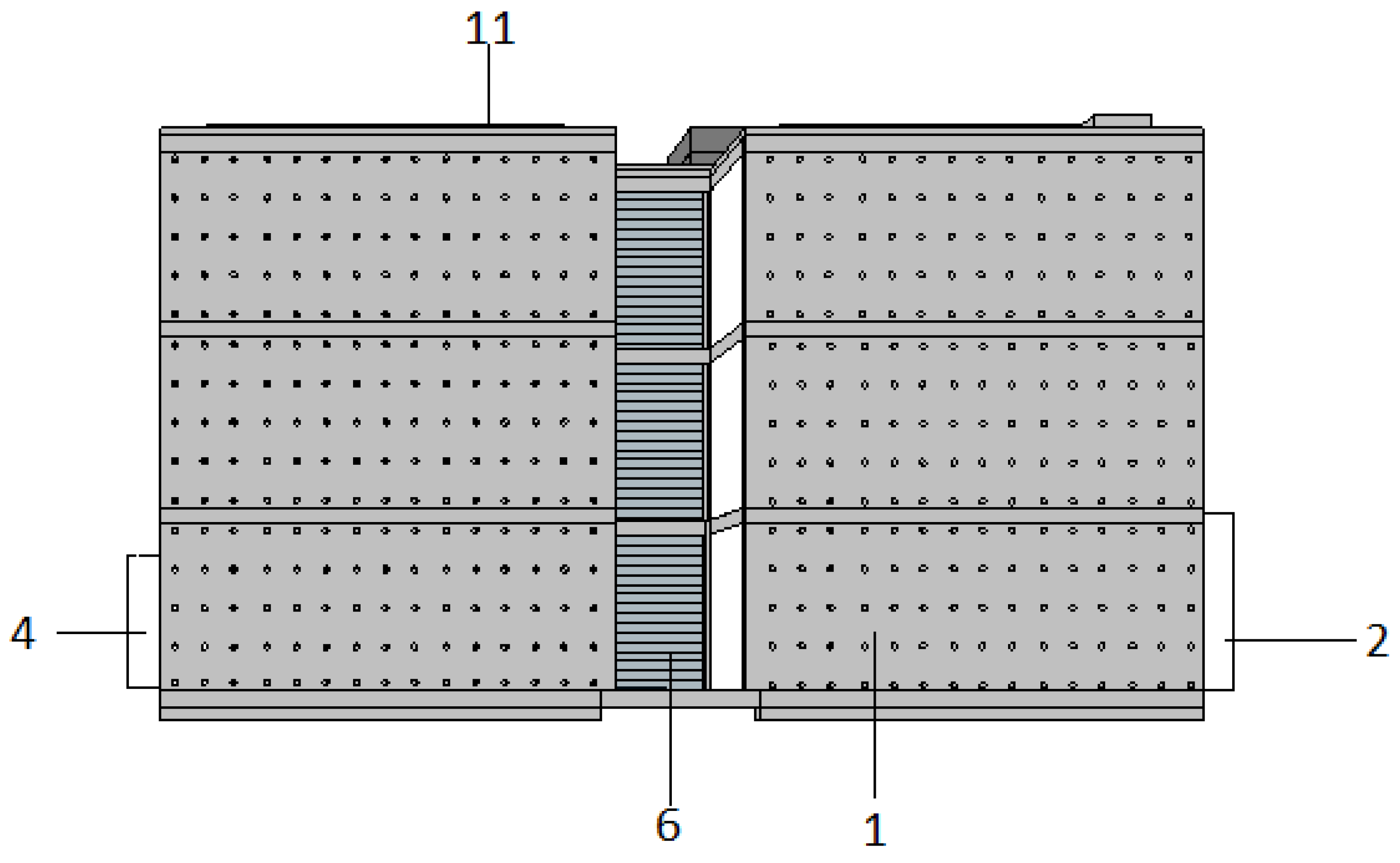
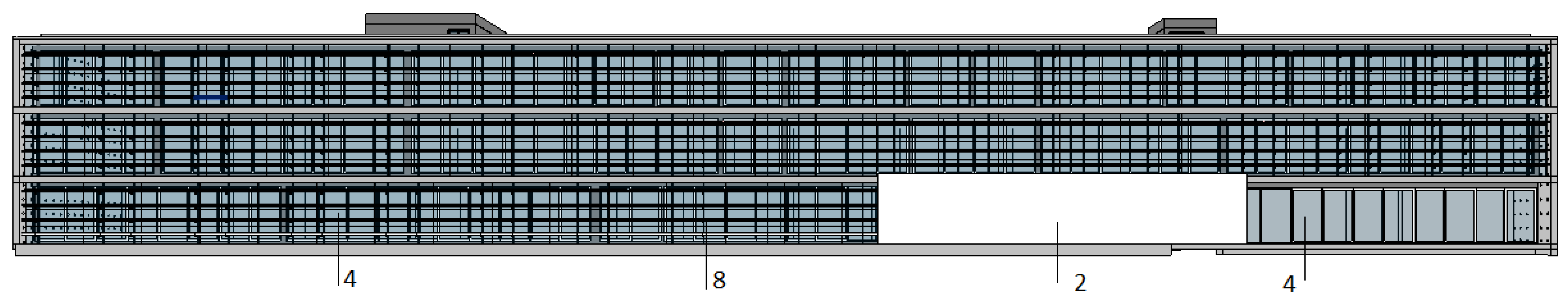
The identification and location of each construction system are indicated in the plant (
Figure 6), in the main facade—NE—(
Figure 7), and in the SE facade (
Figure 8). The construction systems are identified using the numbers defined above.
The degradation functions used to test and adapt the data field in each construction system include loss in performance as the dependent variable and time as the independent variable; they are the Gompertz, Weibull, Potential, second- and third-degree polynomial functions. The R2 score was used as a measure of the fit of the models to the real data. Although this measure is mainly used while working with linear models [
32], it was employed in this work with non-linear models since the trend of the data was approximately linear. The highest R2 score and a decreasing performance curve (ISO 15686-7:2006) [
33] allow the selection of the best curve representing each kind of degradation for each construction system. With this, the predicted year of intervention is presented as well as the root mean squared error of the degradation estimations (RMSE).
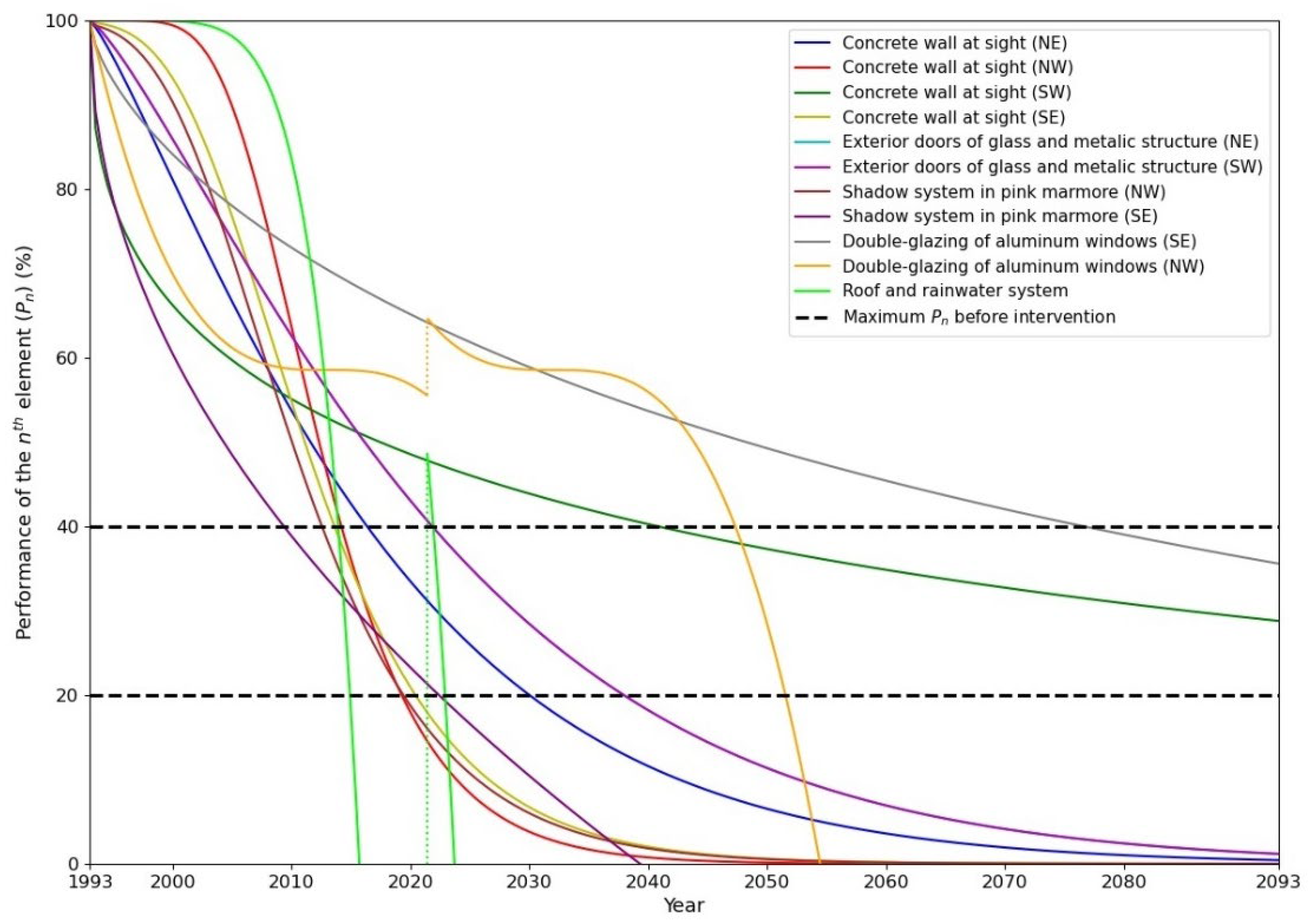
Table 2 presents the curve that best fits each construction system through the condition assessment obtained from the data recorded over the years and its respective R2 score. The curves represent degradation mechanism evolution, taking exposure and orientation into account. This achievement is relevant since the mechanism of degradation of the various elements varies according to the exposure of the construction system, and in this specific case, these adjustments were obtained using actual records since 1993.
The referred curves were plotted for each construction element/system all together in
Figure 9. For better interpretation,
Figure 10,
Figure 11 and
Figure 12 show the degradation curves for each construction system for all orientations and the mean curves of the degradation mechanism that represents each of them. Besides that, the maintenance actions that proceeded over the years were also presented in the degradation curves through an increase in performance in a given year, which is represented by the vertical translation (as dotted lines) as presented in
Figure 9,
Figure 11 (on the right) and
Figure 12. Based on real data, this work has the potential to be applied to other buildings and to be useful for the prediction of the degradation of a general construction system.
Figure 9,
Figure 10,
Figure 11 and
Figure 12 show two thresholds established according to the selected KPI to proceed with the building evaluation. The thresholds represent two important moments during the degradation of the construction system: a threshold of 20 which indicates a near-imminent need for replacement of the construction system, and a threshold of 40 which indicates the need for urgent maintenance actions, as those carried out previously were not enough to correct the existing defects. The functions representing the mean curves of each construction system are presented
Table 3.
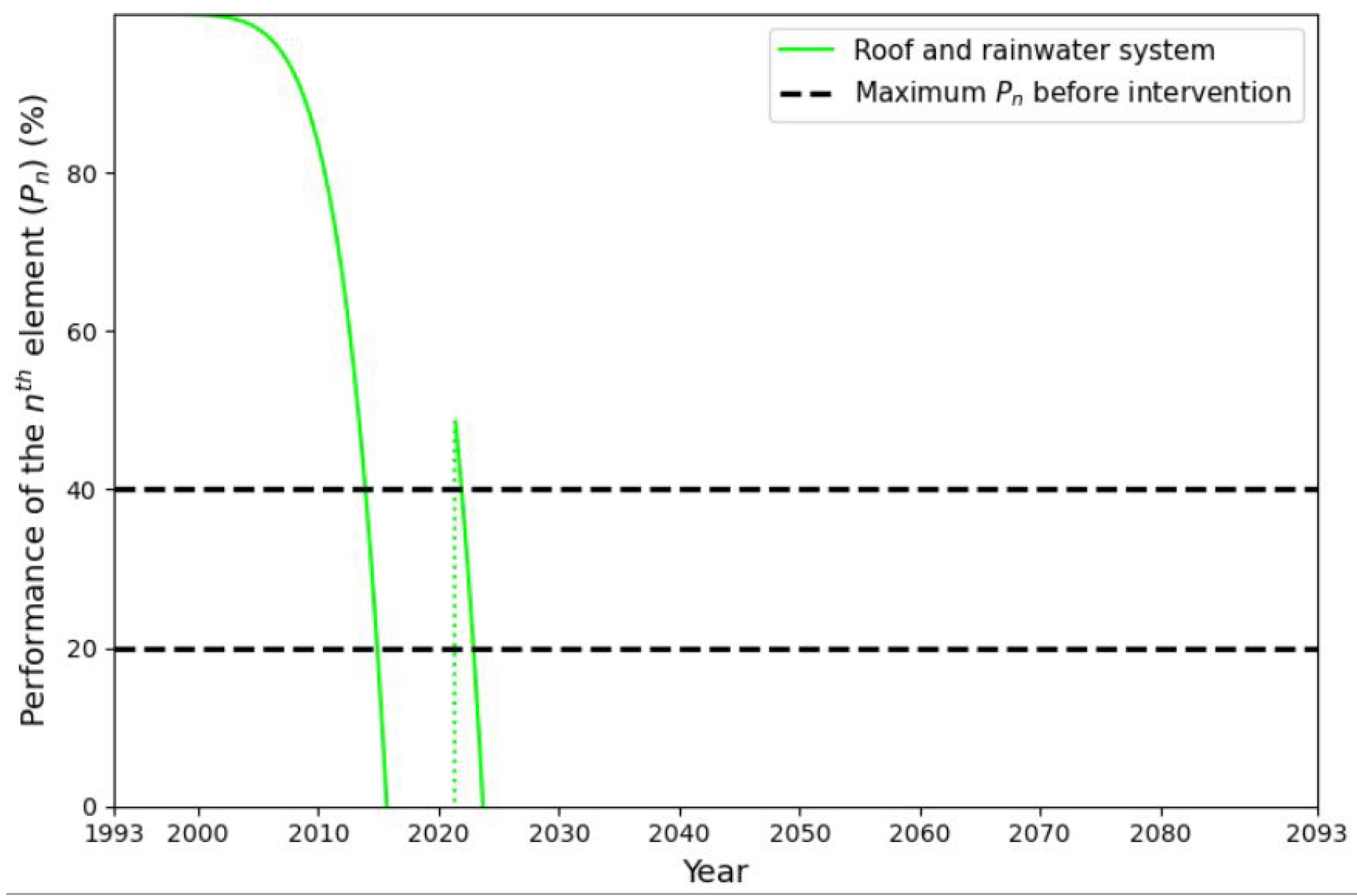
It is interesting to highlight that the function that represents the degradation curve of the roof and rainwater system is the Potential function, as mentioned in
Table 2.
The correspondence of the curve functions with each constructive element allows for the adaptation of the evaluation of the condition decay of a building according to each specific case, which enables the reproduction of a regression model for other buildings. This model is a valuable contribution as a starting point for the automated prediction of georeferenced anomalies linked to the BIM model.
4.3. Discussion of the Results
The multiple series regression was carried out over 100 years. Two thresholds representing the start of the building’s critical condition were established according to the building condition assessment scale from the KPI selected to proceed with the evaluations. The threshold representing the condition assessment of 20 was implemented, making it possible to recognize the urgent situations for which refurbishment or replacement actions must be prioritized to restore the initial building performance. The threshold of 20 draws attention to the critical state of the conservation of elements, and it establishes a priority to avoid catastrophic costs and damages in the surrounding materials. The threshold of 40 draws attention to systems that have considerable defects that jeopardize the continuity of operation. The degradation curves obtained for each construction system based on real data are characterized by decreasing performance over the years. The shape of the curves represents the deterioration mechanism that changes its intensity over time. Each curve was developed for each construction system based on the real values of degradation over the years. It is important to note that the curve corresponding to the element exterior doors of glass and metallic structure (NE) is the same as the curve corresponding to the element exterior doors of glass and metallic structure (SW), since its data was not sufficient to yield the best curve parameters. It is important to note that they correspond to the same element, but with different orientations. The Potential curve has the most adequate shape to represent the degradation of the roof and rainwater system, and it is characterized by a fast decrease in performance. It indicates that the performance level would have gone to zero before the year in which the maintenance was carried out, in 2021. This shape can be justified with the lack of inspections and evaluations of the roof and rainwater system between 2014 and 2021. In 2021, a maintenance action was performed which restored the condition of the construction system. The decreasing performance is related to the ageing of the materials, loss of functionality, and pollution. The curve that belongs to the double glazing of aluminum windows (NW) assumes a decreasing performance and then a punctual increase in performance due to the maintenance action performed in 2021, which restored its functionality.
Figure 6 presents that two elements do not overcome the threshold of the condition in 100 years: the double glazing of aluminum windows (SE) and concrete wall at sight (SW). Although they are significant construction systems exposed to climate and pollution, their orientation allows them to not develop microorganisms or another degradation mechanism.
The elements double glazing of aluminum windows (SE)(NW), a concrete wall at sight (SW)(NE), exterior doors of glass and metallic structure (SW)(NE), and a shadow system in pink marble (SE) are represented by a concave degradation curve. This shape translates to a fast loss in performance and then the decay slows down over time, which, according to the orientation, may be due to rain exposure in the NW and NE facades and pollution in the SE and SW facades. The elements roof and rainwater system, concrete wall at sight (SE)(NW), and shadow system in pink marble (NW) assume a convex degradation curve, which indicates an unpronounced performance loss at the beginning of the service lives of the components. But once it starts to present degradation, the performance loss is quick, which may mean that the construction system has a protective layer, and after its degradation, the loss in performance is significant [
34]. The roof and rainwater system is the most exposed to the climate, but the construction system is not susceptible until it suffers the first defects. The concrete wall at sight is more susceptible to degradation once it starts, due to the geometric shape that the wall assumes, accessibility to users, and the join of several materials.
Feeding the model with current and updated data every year would be an advantage to adjusting the shape of the curves to the degradation mechanism and improving the prediction ability of the model.
The statistical indices are analyzed, such as the root mean squared error (RMSE) [
35], which enables the conclusion of the efficiency and accuracy of the model. The RMSE makes it possible to obtain the difference between the measured and simulated values [
36]. According to this author, the lower the RMSE, the better the model performance.
With the intersection of the degradation curves and the thresholds defined, the moment at which to apply the maintenance action—the year of intervention (1)—when the degradation curve intersects the threshold 40, and the refurbishment/replacement intervention—the year of intervention (2)—when the degradation curve intersects the threshold 20, as well as the accuracy of the degradation prediction determined using the RMSE, were obtained for each construction system and orientation, as presented in
Table 4.
The closer the RMSE is to zero, the more accurate the model is, since it indicates a better fit of the model’s predictions.
Table 4 presents the likely year in which to proceed with the intervention before the condition of the components starts to deteriorate and consequently affect the surrounded materials. So, according to
Table 4, the maximum RMSE is 48.36, which represents the average error that the model’s prediction has in comparison with the real values for the construction system a concrete wall at sight (NW).
5. Conclusions
New buildings are uncommon for most organizations, which makes the evaluation and management of the built environment a valuable activity able to address sustainable practices. A sustainable built environment can only be achieved using digitalization, new construction techniques, and innovation. On the other hand, a BCA is essential to assess building durability. So, bridges must be built in the sector to unite this activity and technology to pursue a more efficient assessment technique.
This study proposed a programming framework for the identification of building anomalies and the prediction of building degradation using ML/DL and mathematic algorithms. The framework was composed of the DL pipeline based on computer vision algorithms to detect the degradation of a component and a regression model to predict the future degradation of a component accurately. The extent of the damage was not explored nor included in the automatized tool, which can be carried out in future development. The second part of the work consisted of the multiple series regression models, based on past evaluations of the condition of the components to predict the most likely year for the future degradation of the components. This part of the work involved several degradation curves and functions, which were tested, and each building component was analyzed. The mathematical functions representing each degradation curve for each construction system, according to its orientation and based on real records, are presented and can be reproduced and applied to other building typologies. Besides that, two quantitative thresholds of 20 and 40 were established. The first one (20) means that the component is on the verge of becoming inoperable and requires reparation or replacement. The threshold of 40 prioritizes the elements that are on the verge of having irreparable defects that compromise their operability and can make their maintenance no longer possible. So, for this threshold, it is essential to prioritize maintenance actions and to extend the service life of the construction systems, otherwise conservation may be irreparable and may carry catastrophic costs. Moreover, the maintenance actions applied can be represented in this regression model to be presented in the degradation curve by a change in its path, being a valuable novelty of this work.
Although these models are still separated, both models are automated tools useful for the detection and prediction of building degradation. Moreover, connecting with each other is valuable since it may be a starting point for the automated detection and prediction of georeferenced anomalies linked to the BIM model. This study can also be reproduced in other buildings of the public building stock, with an increase in the dataset of the ML/DL algorithm, and also through updating the evaluation of the condition of a building according to each specific case.
As future developments, the connection between the DL and regression models and Revit will be made, and the correspondence of each anomaly will be made using georeferencing, so all the information related to the building anomaly can be stored and linked to the model in a unique 3D platform. For this purpose, an online app will be deployed and linked to Revit software as an add-in. However, it is interesting to note that despite relying on real data, this study does not account for the future effects of climate change, which may influence the results of future predictions to be obtained, which can be considered as a limitation. However, along with the building inspections, more data will be introduced, and the degradation curve will be updated based on it. So, it provides a programme of checks and actions used to monitor and resolve any critical issues.


