Abstract
Monopole communication towers play an irreplaceable role in modern communication systems. Because of its high flexibility, lateral loads control the deformation of a monopole communication tower. Dynamic displacement can be used to describe structural vibration characteristics and real-time deformation situations. Therefore, this article proposes a monopole communication tower deformation monitoring method based on multi-source data fusion using dynamic displacement as the evaluation indicator. This method calculates the strain displacement using the strain-mode superposition methodology. Then, the strain displacement and acceleration obtained are processed using Kalman filtering technology to reconstruct the real-time displacements of the monopole communication tower. The effectiveness of this method was verified using numerical simulations and model experiments, respectively. In addition, parametric analysis shows that this method is suitable for processing multi-rate data, has good noise resistance in strong noise environments, and can effectively reconstruct the displacement near the tower bottom. The results indicate that the method has favorable robustness and can accurately reconstruct low-frequency and high-frequency displacements of the monopole communication tower.
1. Introduction
With the development of communication technology in modern society, the number of communication towers is growing rapidly [1]. According to the different structural characteristics and force forms, communication towers can be divided into space truss towers, monopole towers, and cable towers. Among them, monopole communication towers are most widely used because of their small footprint, light structural weight, and fast construction speed. As typical high-rise structures, monopole communication towers have high flexibility and are prone to vibration and lateral displacement under lateral loads [2,3,4]. In recent years, there have been multiple collapses of communication towers both domestically and internationally [5,6,7], making it necessary to conduct health monitoring on them. Dynamic displacement can intuitively reflect the deformation of the structure [8,9], so monitoring lateral displacement is significant for deformation monitoring and vibration control of monopole communication towers [10,11].
Monopole communication towers are cantilever structures with large slenderness and low stiffness. The horizontal displacement of the tower top plays a controlling role in structural deformation. Therefore, researchers have conducted extensive research on dynamic displacement monitoring of cantilever structures. Celebi [12] successfully measured the top displacement of a bottom-fixed steel bar and a 44-story building using GPS technology. However, the sampling rate and accuracy of GPS are low, making it difficult to effectively monitor high-frequency displacement under dynamic response. Moschas et al. [13] mounted a total station (TS) on a 30 m transmission tower and observed the tower top displacement on strong windy days. Although a TS has high accuracy, it can only measure point displacement, which makes it difficult to fully reflect the deformation of the structure. Lee et al. [14] installed a laser displacement meter in an offshore wind turbine tower to achieve deflection and damage monitoring of the turbine blades without contact. Since the light source of laser displacement meters is easily affected by the working environment, it is difficult to apply it directly to long-term outdoor monitoring structures such as monopole communication towers.
The above research directly measures the dynamic displacement using different displacement sensors. However, in some cases, directly measuring dynamic displacement can be challenging or even impossible. Therefore, displacement reconstruction methods have emerged. The displacement reconstruction method [15,16] is a method of indirectly deriving displacement with mathematical relationships using physical quantities related to displacement. Commonly used physical quantities include strain [17], acceleration [18], and inclination angle [19]. Bang et al. [20] deployed an FBG sensor array on a 70 m wind power tower and derived the dynamic displacement of the tower top using strain time history. However, the cost of this monitoring method is high and the packaging process of FBG sensors is also complex. Li et al. [21] reconstructed the static and dynamic displacements of an offshore wind turbine tower top using strain based on the inverse finite element method (iFEM). However, the iFEM requires optimization of sensor placement as the measured structure changes and has only been validated using numerical simulations. Liu et al. [22] proposed an acceleration-based horizontal displacement measurement method for offshore platforms. The dynamic displacement of the platform and column was accurately measured using vibration table experiments, but the accuracy of acceleration decomposition needs to be ensured. Wu et al. [23] used the inclination angle as a physical quantity combined with an improved IM-DINSAR algorithm and residual interferometry to estimate the tilt displacement of a transmission tower top. However, because of the impact of measurement accuracy and data update rate, this method is only suitable for long-term monitoring and reconstruction of low-frequency displacement.
Since actual structural health monitoring generally uses a combination of multiple sensors, each type of sensor contains different information. Considering the limitations of the single physical quantity displacement reconstruction method, researchers have further proposed a displacement reconstruction method based on multi-source data [24,25,26,27]. Wang et al. [28] accurately reconstructed the vibration response of two 65 m wind turbine towers using Kalman filtering techniques to process the displacement and velocity responses. Park et al. [29] successfully estimated the dynamic deflection of the Sorok bridge by integrating strain and acceleration information. Zhu et al. [30] proposed a Kalman filtering algorithm suitable for super high-rise structures and applied it to the deformation monitoring of Canton Tower.
Although the displacement reconstruction method based on multi-source data is generally superior to the single physical quantity displacement reconstruction method, there are still problems such as dependence on observed displacement, inability to process multi-rate data, and excessive use of sensors [31,32,33]. At present, there is relatively little research on the deformation monitoring of monopole communication towers, and the relevant theories and methods are still immature. Therefore, this article proposes an algorithm based on multi-source data suitable for displacement reconstruction of monopole communication towers. This algorithm can calculate low sampling rate displacement based on measured strain, which is more consistent with actual structures. Then, multi-rate Kalman filtering technology is used to fuse the corresponding strain and acceleration information to obtain high-precision reconstructed dynamic displacement. To examine the performance of the algorithm, the results obtained from numerical simulations and modeling experiments are parametrically analyzed, respectively. Finally, the conclusions of the research are given.
2. Displacement Reconstruction Method for Monopole Communication Towers
2.1. Strain-Mode Superposition Methodology
Considering the characteristics of a monopole communication tower, it is simplified as a thin-walled cantilever beam. In the online elastic deformation stage, strain and displacement can be represented by the superposition of vibration modes as:
where and denote the strain and displacement of position x at time t;
and are the jth order strain mode and displacement mode; represents the modal displacement; and k is the mode order considered. The strain and displacement modes correspond to each other.
According to Equation (1) and the least squares method, the approximate solution for modal displacement can be obtained:
where p is the number of measurement points, q represents the order of the considered modes, and T represents the transpose of the matrix or vector. According to Equation (3), solving the displacement response requires first calculating the strain shape function . The stochastic subspace identification (SSI) method can directly deal with the dynamic response of structures without relying on theoretical vibration modes. Therefore, the SSI method with better applicability is used to identify the strain mode shape of the structure. Due to space limitations, the identification process of this method will not be introduced in detail. Readers can refer to the theories of Overschee and Moor [34].
Furthermore, assuming that the measurement point is located at a distance y from the neutral layer, according to Euler beam theory, it can be concluded that:
where denotes displacement; represents strain; indicates bending moment; and is bending stiffness.
Substituting Equations (1) and (2) into Equation (4), eliminating the modal displacements at both ends, and integrating twice, the first-order displacement modal function can be expressed as:
Since the monopole communication towers are cantilever structures, the two integration constants B and C are both 0. According to Equation (5), the first q-order displacement vibration mode values are calculated and then assembled into a displacement mode matrix :
The dynamic displacement can be derived from the modal displacements and the displacement modal matrix:
2.2. Displacement Reconstruction Algorithm Based on Multi-Source Data
The above strain-mode superposition methodology can only obtain dynamic displacements with the same sampling rate as the strain. However, in practical engineering, strain is usually sampled at low frequencies, while acceleration is sampled at high frequencies. Data fusion technology [35] can improve the confidence of data and enhance the fault tolerance and adaptive ability of the system by integrating heterogeneous data. Therefore, this article proposes a multi-source data fusion algorithm for strain sensors and accelerometers to obtain high-precision displacement.
The improvement of the proposed algorithm is that the strain displacements derived from the measured strain modes are used as observations, which is more applicable and more in line with the actual structure than the method of deriving the strain displacements using theoretical models. The actual data obtained are discrete, so a discretized state space model is given:
where A denotes the discrete-time state transfer matrix; represents the control matrix; and indicates the noise matrix.
According to Equation (8), the predicted one-step state vector is:
where denotes the l − 1th time-step state vector; represents the lth time-step state vector predicted at step l – 1; and the covariance array of the process can be expressed as:
where indicates the l − 1th time-step covariance matrix; is the lth time-step covariance matrix predicted at step l − 1; and N denotes the random noise covariance matrix, which is calculated from the control matrix and the acceleration measurement noise covariance :
Based on the measured strains, the strain-mode superposition methodology can be utilized to restore real-time displacements at any location in the structure. The strain-derived displacement can be used for Kalman filtering measurement updates. Assuming that the displacement response is obtained at the jth time step, the displacement during the measurement update process can be expressed by the observation equation:
where denotes the observed displacement and H is the observation matrix. During the measurement update process, the state estimation vector and state estimation covariance matrix can be represented as:
where represents the jth time-step Kalman gain matrix. The formula is as follows:
where denotes the measurement noise variance during the observation.
After completing the above calculation process, the reconstructed displacement is finally obtained. The calculation flow of the algorithm is shown in Figure 1.
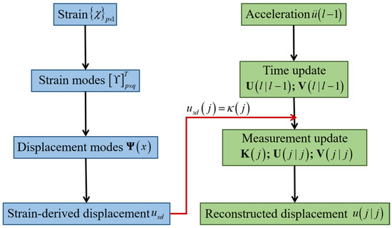
Figure 1.
Calculation flow of the algorithm.
3. Numerical Simulation Validation
3.1. Numerical Model
Because of limited space, this article only verifies the effectiveness of the algorithm applied in numerical simulations and model experiments. A 30 m high monopole communication tower of China Tower Corporation Limited is taken as the prototype. Since the model experiment does not involve comparison with the original structure, only the geometric dimensions need to be considered when determining the scale. According to the geometric dimensions of the monopole communication tower, and for comparison with the experimental model, the geometric scale ratio is determined as λL = 1/20. The numerical model of the monopole communication tower is established using ANSYS software. Among them, the tower body and lightning rod are simulated using Beam 188 elements. The top cover plate of the tower is simulated using Solid 185 elements. The auxiliary structures, such as antenna poles and equipment, are simulated using Mass 21 elements and applied in the form of concentrated loads at the horizontal nodes of each section. The bottom of the model is fixed. The model tower is a 1.5 m round tube. The outer diameter is 40 mm, and the wall thickness is 2 mm. The lightning rod at the top of the tower is 12 mm in diameter and 0.3 m in height. The lightning rod and the tower are connected by the top cover plate. The elastic modulus is 210 GPa, and Poisson’s ratio is 0.3. Considering the cables, antenna poles, and auxiliary structures on the monopole communication tower, the density is set at 8000 kg/m3.
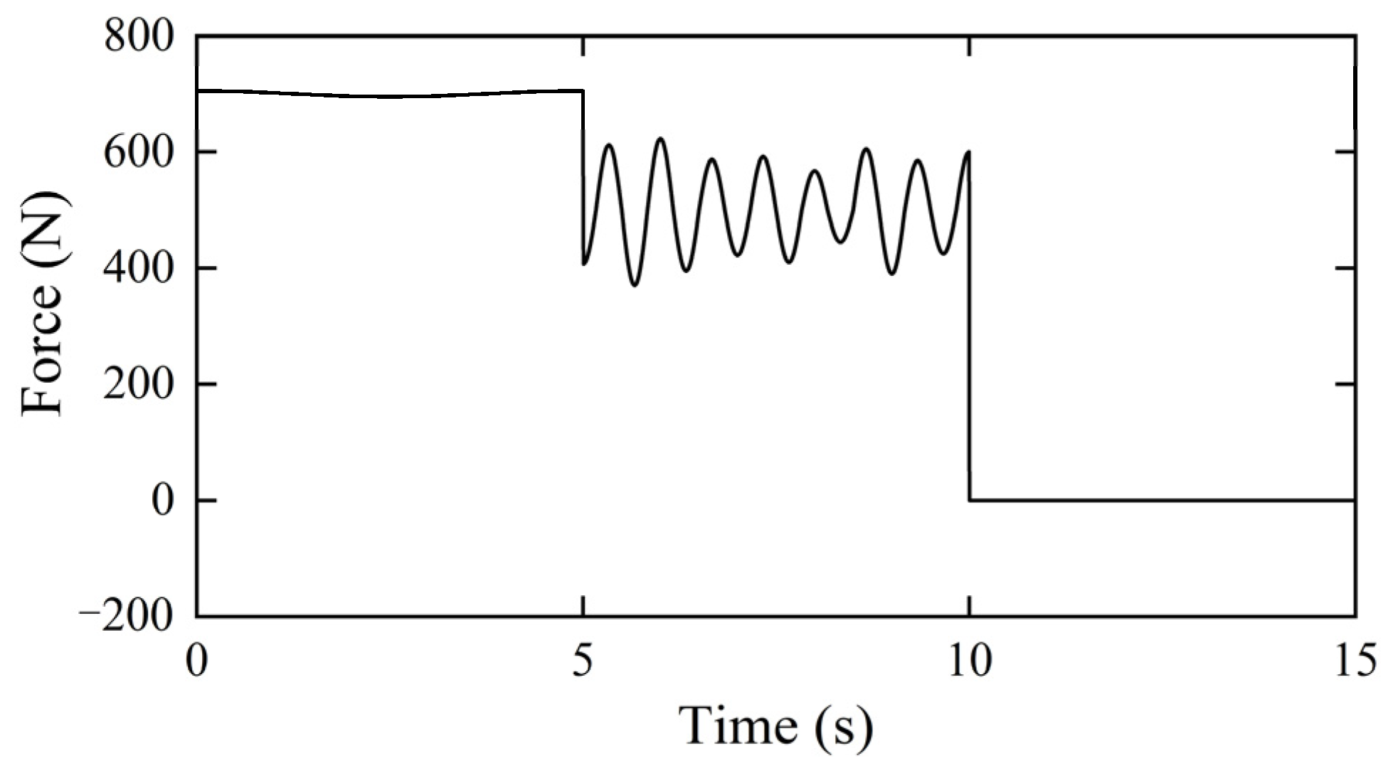
The excitation of the model is set along the X-direction for 15 s. The loading point is located at the top of the lightning rod. The time history of external excitation is shown in Figure 2, including pseudo-static excitation, random vibration excitation, and pulse excitation that generates a free attenuation response.
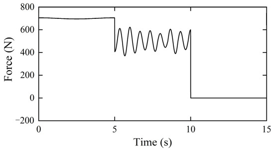
Figure 2.
Time history of the external excitation.
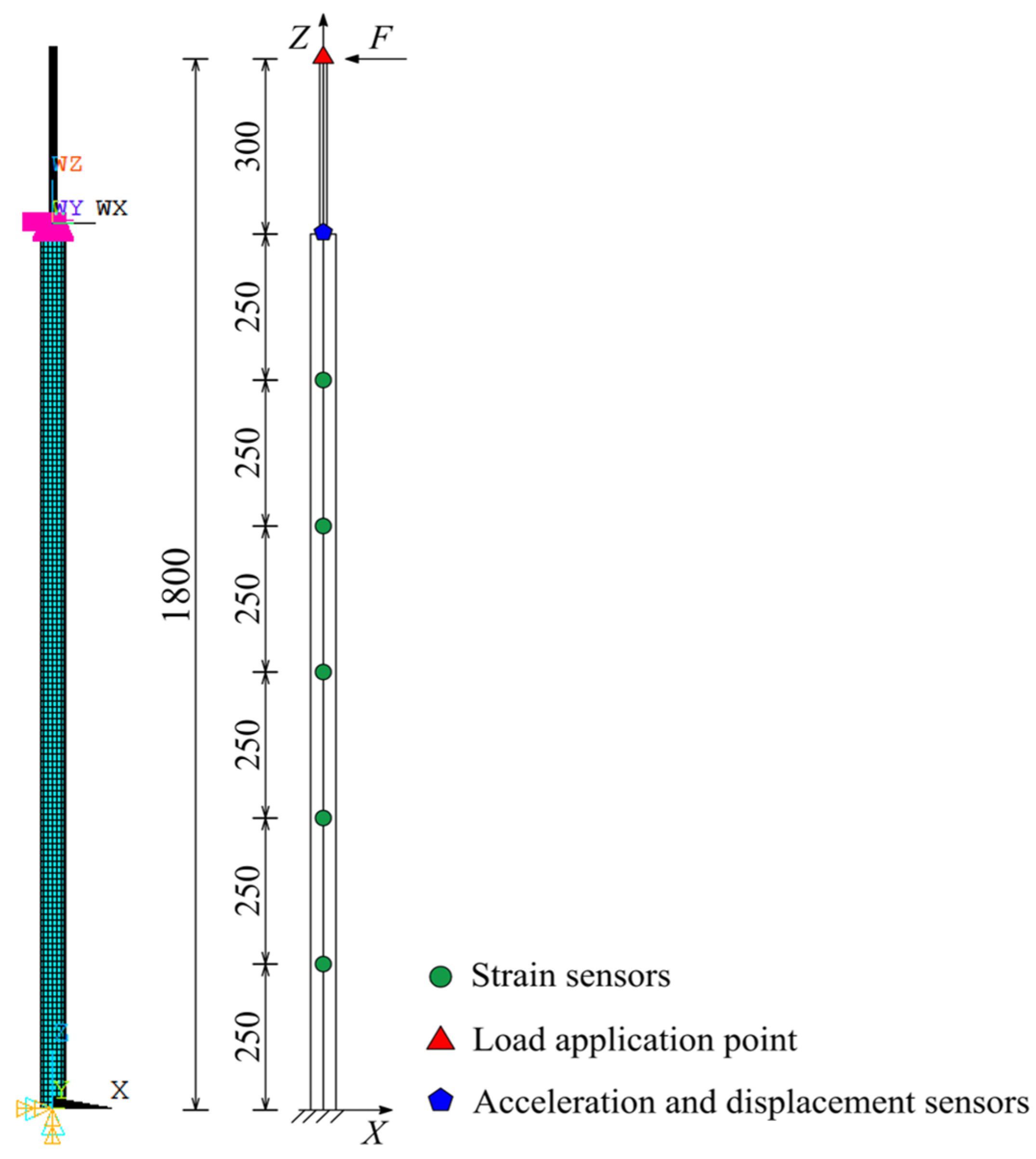
Considering the size and vibration characteristics of the model, five strain measurement points were uniformly set up from top to bottom along the tower body of the model. The top of the tower was set as the extraction point for the displacement and acceleration responses. The sampling rate for acceleration and displacement is 1200 Hz, and strain is sampled at 300 Hz. The numerical model, observation points, and loading point positions are given in Figure 3.
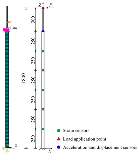
Figure 3.
Numerical model and observation points.
3.2. Comparison of Reconstructed Displacements
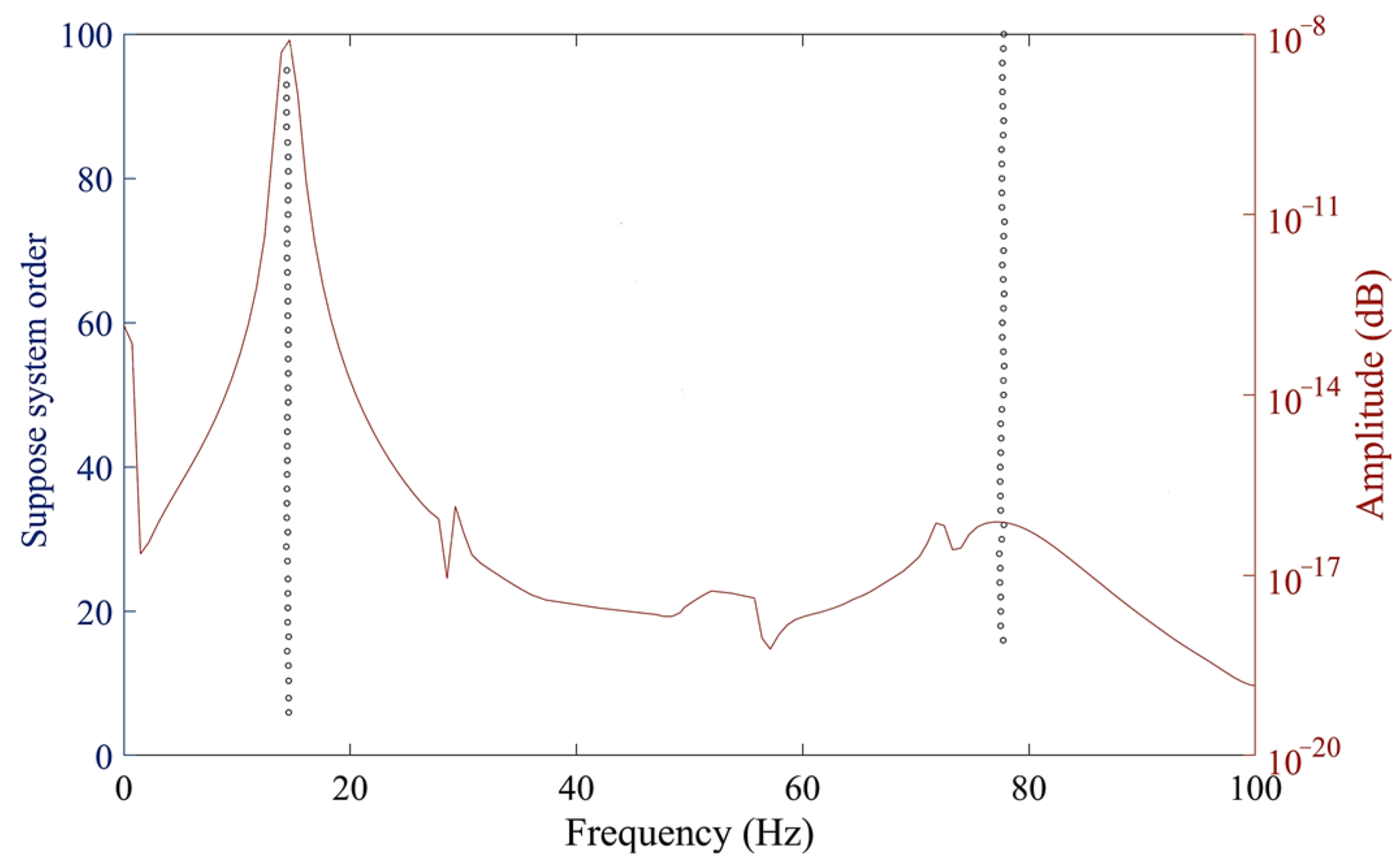
The strain and acceleration response time histories derived from ANSYS software were processed with the SSI method. The stability plot and spectral curve were acquired, as shown in Figure 4. The circles in the figure represent strain mode points with stable solutions, and the orange curves represent the spectral curve. From Figure 4, it can be seen that the first two orders of strain modes of the structure contributed the majority of the vibration energy, so the extraction of the first two strain modes can meet the requirements.
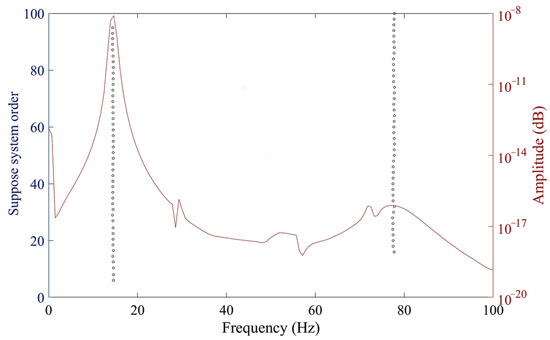
Figure 4.
Stability plot and spectral curve (numerical simulation).
A comparison between the first two frequencies corresponding to the extracted stable axis and the ANSYS modal analysis results is shown in Table 1. Table 1 shows that the frequency and modal analysis results obtained using the SSI method for the strain time history are consistent, with a maximum error of only 0.74%.

Table 1.
Comparison of the first two-order frequencies (numerical simulation).
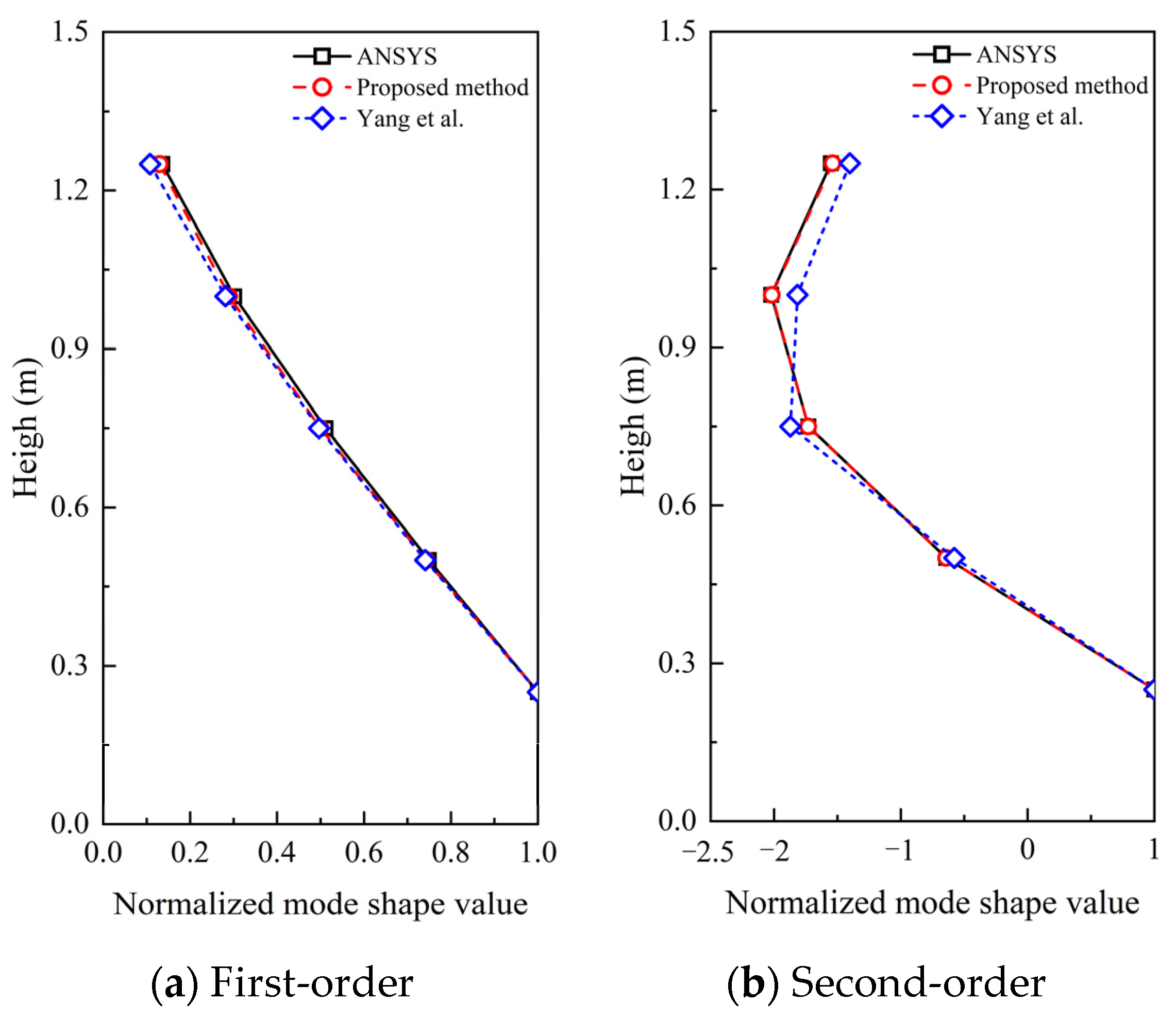
As shown in Figure 5, the SSI-derived strain mode shapes are compared with those obtained by ANSYS and Yang [36]. It can be seen that the first-order mode shapes calculated using Young’s method approach the theoretical values, but the second-order error significantly increases. The recognition results of the methods used in this article are all close to the theoretical values. This is because the dynamic displacement spatial resolution of the method of identifying modal information with photography is low, and the recognition process is easily affected by environmental noise. The SSI method does not rely on expensive digital imaging systems and has low cost, strong robustness, and broader application space.
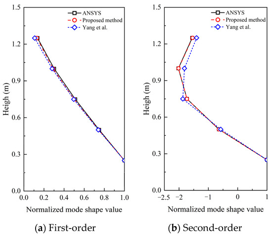
Figure 5.
Comparison of strain mode shapes calculated using different methods [36].
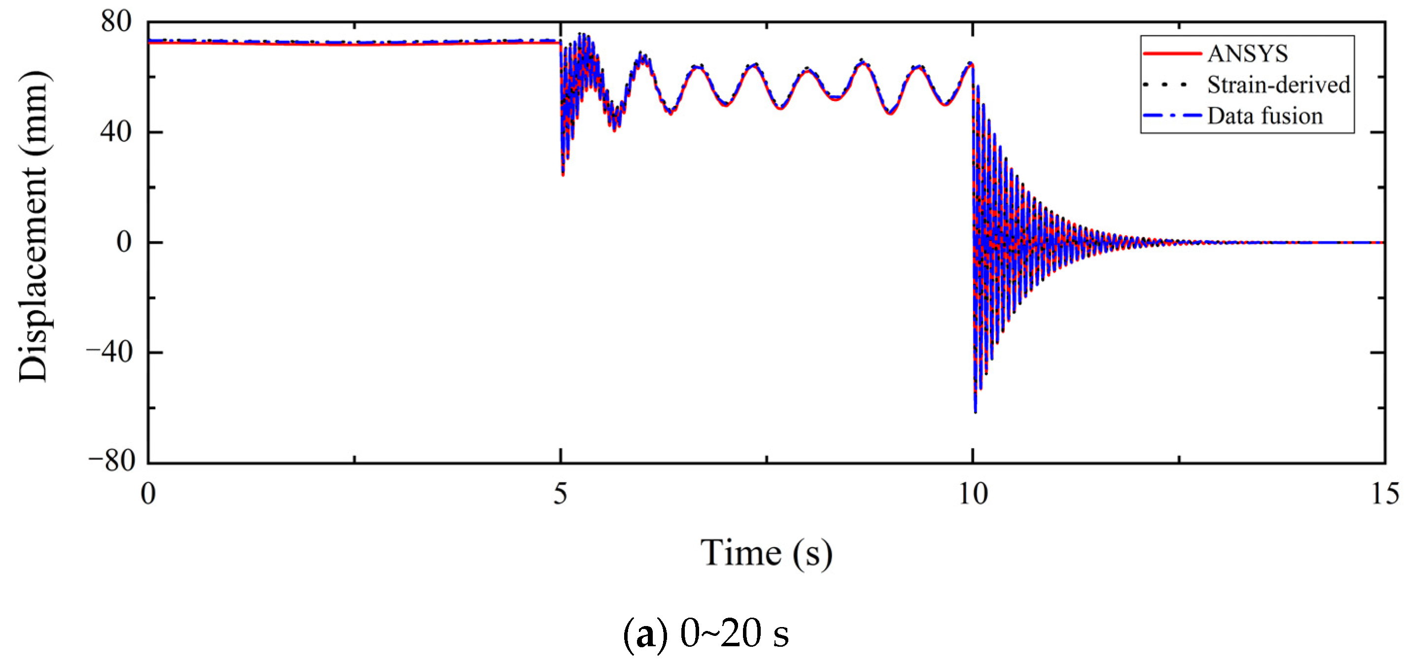
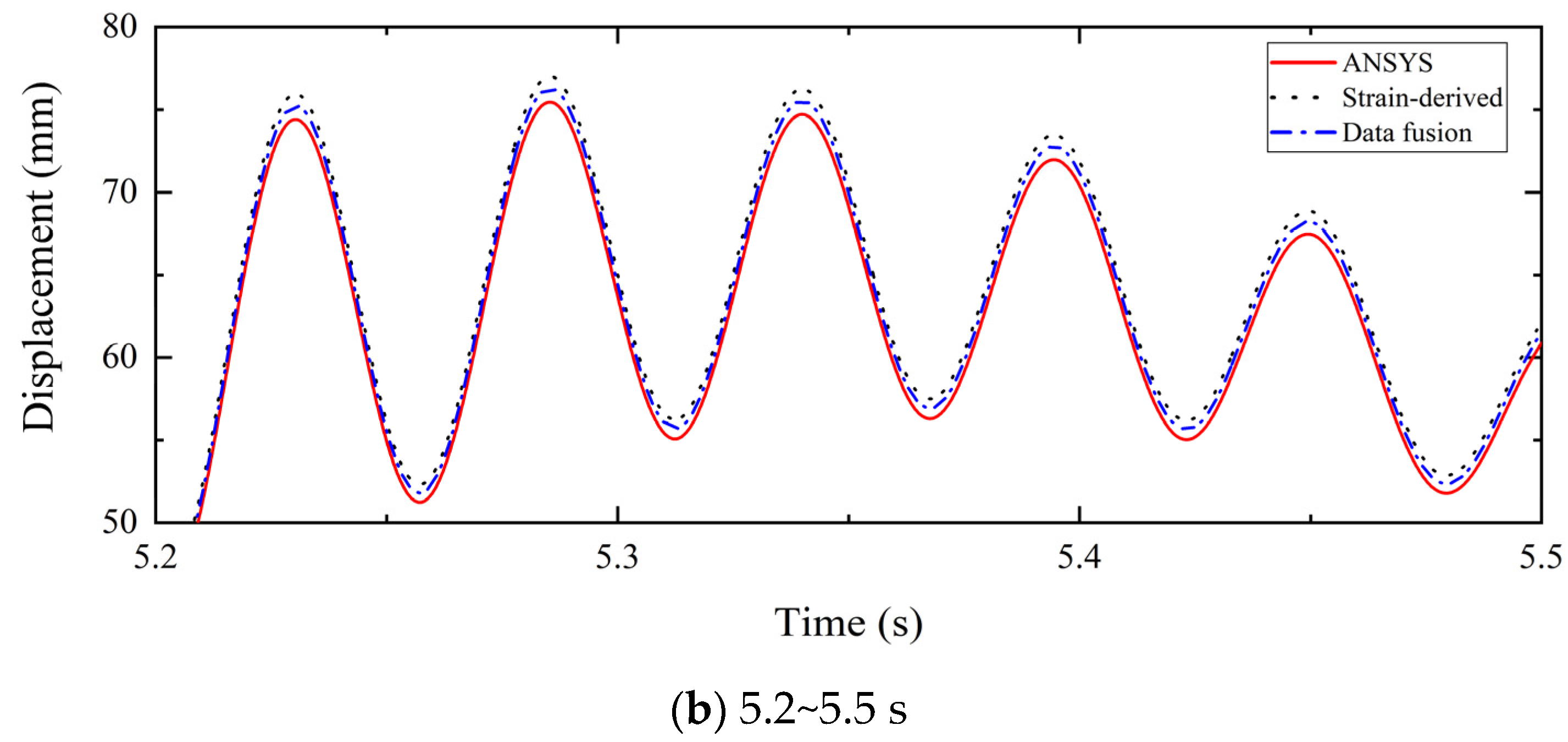
We calculated the strain-derived displacement and data fusion displacement and compared them with the displacement extracted with ANSYS. Figure 6 shows that the reconstructed displacements of the two methods are in good agreement with the theoretical displacements. In the low-frequency excitation stage, the reconstructed displacements of the two methods almost coincide. However, in the stage of random vibration excitation, observing the locally enlarged images from 5.2 to 5.5 s reveals that the multi-source data fusion displacements are closer to the theoretical displacements. This indicates that the proposed data fusion algorithm can not only reconstruct low-frequency displacements but also improve the reconstruction accuracy of high-frequency displacements, which is superior to the strain-mode superposition methodology.
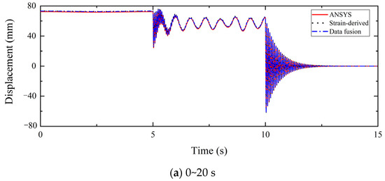
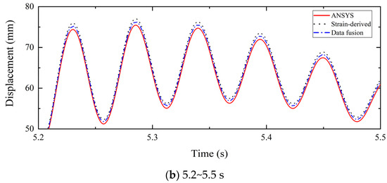
Figure 6.
Dynamic displacement reconstruction using different methods (numerical simulation).
3.3. Parametric Analysis
In the monitoring process of actual structures, there are factors such as different sampling rates of various sensors [37], differences in measurement point positions [38], and environmental noise [39]. Three parameters, the sampling ratio (SR), distance ratio (DR), and signal-to-noise ratio (SNR), are proposed for the above-mentioned influencing factors. Among them, SR = acceleration sampling rate/strain sampling rate. Meanwhile, to quantitatively assess the degree of deviation of the reconstructed displacement from the theoretical/measured displacement, assuming that N data are collected, the error indicator η is defined as:
where ur is the reconstructed displacement and ut represents the theoretical displacement calculated using ANSYS in numerical simulations and the measured displacement in model experiments.
The working conditions designed based on these parameters are given in Table 2.
Table 2.
Working condition design (numerical simulation).
The excitation points and strain response extraction points applied to the model are the same as those in Figure 3. Four acceleration and displacement extraction points were added along the height of the numerical model at 0.3 m, 0.6 m, 0.9 m, and 1.2 m, respectively. According to Table 2, the same artificial white noise was added to the acceleration and strain responses during the calculations. To save space, subsequent analyses are given only as the displacement time–history plots with the largest errors in the influence factor.
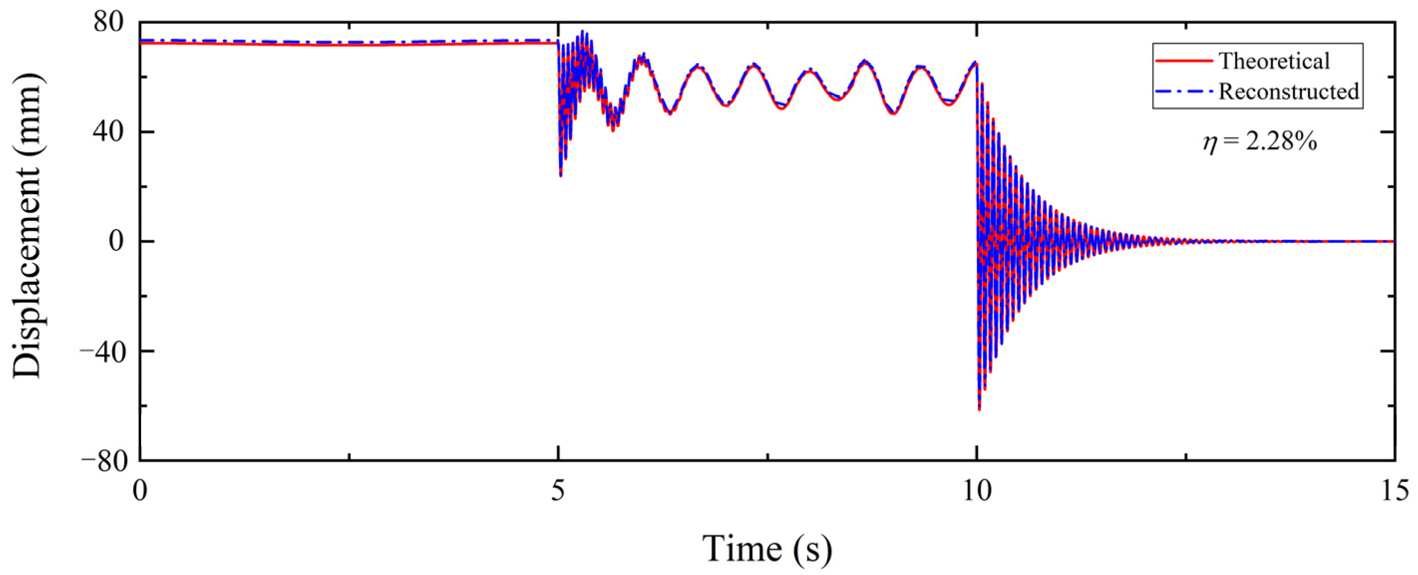
Figure 7 shows the comparison of numerical simulation displacement reconstruction when SR = 100. Compared with Figure 6, the precision of the reconstruction displacement decreases due to the increase in the SR, which leads to a longer measurement update time step, resulting in less strain-derived displacement during the measurement correction process and an increase in reconstruction error.
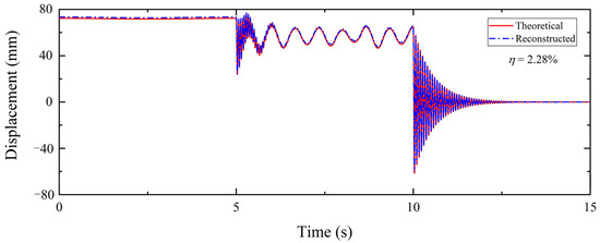
Figure 7.
Comparison of numerical simulation displacement reconstruction (SR = 100).
Table 3 shows the η under different SRs. As the SR increases, the rate difference between the two data increases, and the reconstructed displacement error also increases gradually. However, when the SR reaches 100, η is only 2.28%, indicating that the multi-source data fusion algorithm is applicable to high sampling ratios.
Table 3.
η under different SRs (numerical simulation).
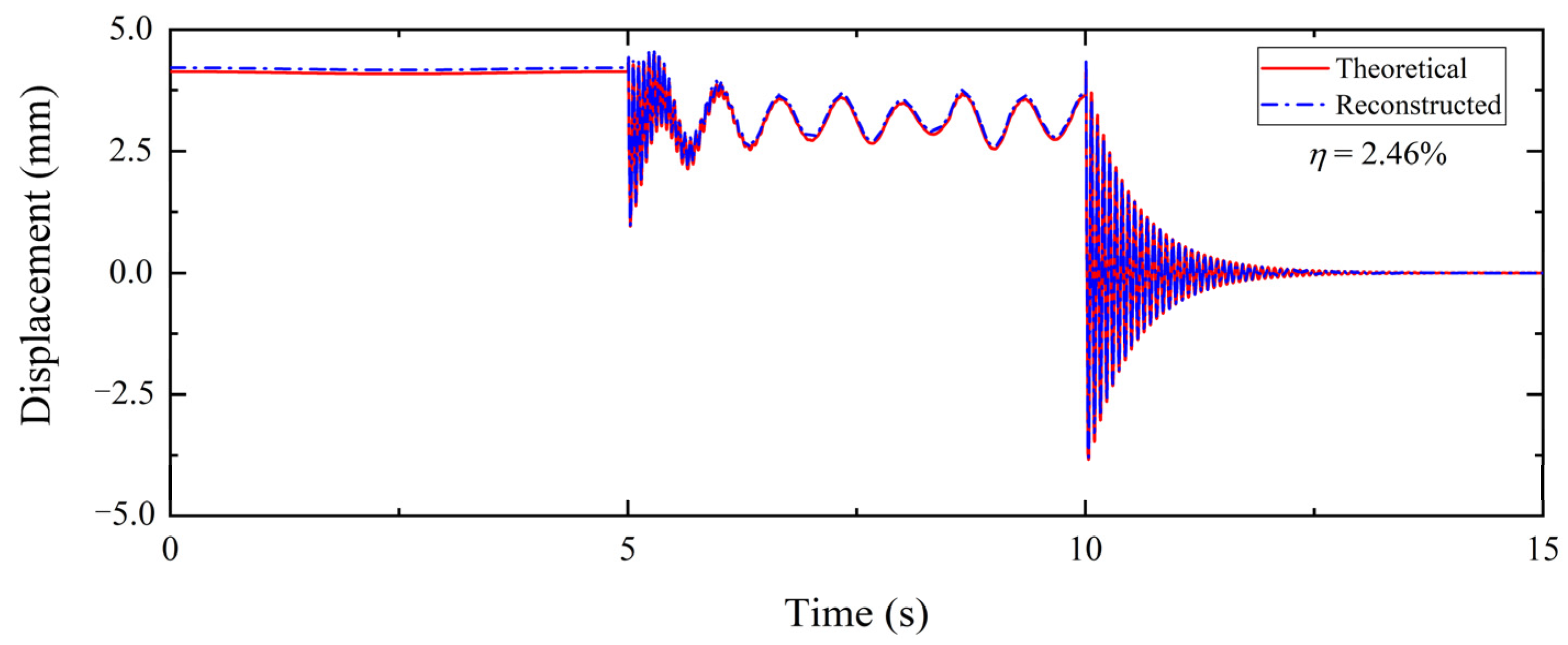
For the cantilever structure, DR = height of measurement point/height of structure, which is used to reflect the proximity of the measurement point to the fixed end. The placement of sensors and the boundary constraints of the structure can also have an impact on displacement reconstruction. Therefore, the measurement points at different positions in the model are analyzed. Figure 8 shows the comparison of numerical simulation displacement reconstruction when DR = 0.2. It can be seen that the accuracy of the reconstructed displacements is reduced. This is because the measurement point is close to the fixed end of the structure and any small measurement error is non-negligible compared to the zero value. As the error is further amplified, it leads to more inaccurate measured strains. The derived displacements also become more inaccurate and ultimately affect the accuracy of the reconstructed displacements.
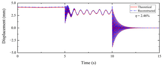
Figure 8.
Comparison of numerical simulation displacement reconstruction (DR = 0.2).
Table 4 shows the η under different DRs. As the distance between the measurement point and the fixed end increases, the error indicator η gradually decreases. For the cantilever structure, as the measurement point is farther away from the fixed end, the displacement response of the structure is larger, which is also favorable for the measurement. For the cantilever structure, as the measurement point is farther away from the fixed end, the displacement response of the structure is larger, which is also conducive to measurement and higher reconstruction displacement accuracy. Nevertheless, η is only 2.46% in the case when DR = 0.2, which indicates that the proposed multi-source data fusion algorithm can effectively calculate the displacements close to the fixed end.
Table 4.
η under different DRs (numerical simulation).
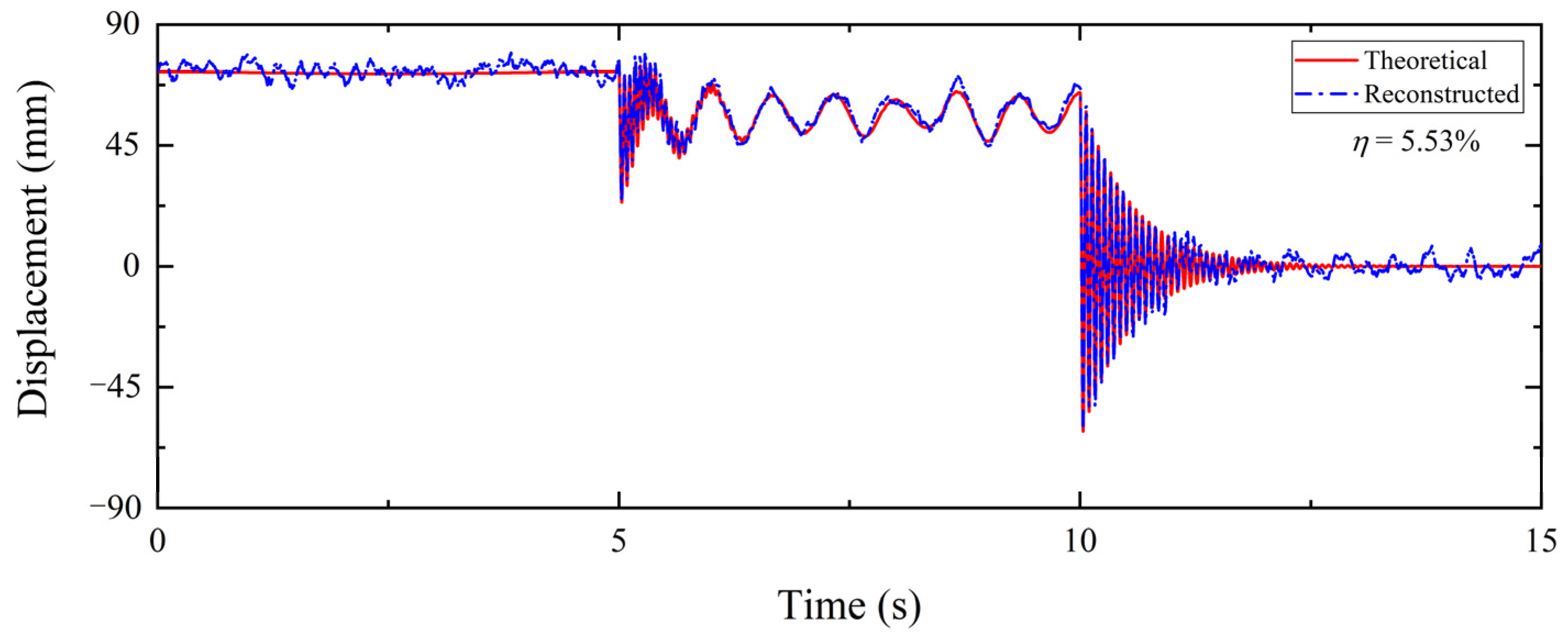
There are environmental noises in practice, so it is necessary to analyze the performance of the proposed algorithm in noisy environments. Figure 9 compares the reconstructed displacements with the theoretical displacements for SNR = 5 dB. Compared with Figure 6, the accuracy of reconstructed pseudo-static displacement and high-frequency displacement is reduced to a certain extent. It is notable that the difference between the reconstructed displacement and the theoretical displacement in the pseudo-static stage increases, while the high-frequency reconstructed displacement and the theoretical displacement still maintain good consistency. This is because of the higher sampling rate of the acceleration response, which can provide more information for the reconstruction of high-frequency displacements. The reconstruction of the pseudo-static displacement mainly depends on the information provided by the strain data, which is basically a single-source information reconstruction. Therefore, the high-frequency displacements reconstructed based on multi-source information are more accurate at the same noise level. Meanwhile, the reconstruction error increases significantly in the late stage of free attenuation. The reason is that the displacement response is very small in this stage, so the error increases in the strong noise environment. After all, η is merely 5.53%, illustrating that the proposed algorithm is still reliable.
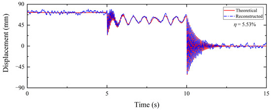
Figure 9.
Comparison of numerical simulation displacement reconstruction (SNR = 5 dB).
Table 5 shows the η under different SNRs. As the SNR increases, the error indicator η gradually decreases. This is because the noise level decreases with an increasing SNR, and the reconstruction displacement accuracy is also improved. When the SNR decreases to 5 dB, η is only 5.53%, proving that the proposed algorithm has strong noise resistance.
Table 5.
η under different SNRs (numerical simulation).
4. Experimental Verification
4.1. Experimental System
To examine the application of the proposed algorithm in real structures, steel was machined into a monopole communication tower model for model experiments. The dimensions and material parameters of each part of the experimental model are the same as those of the finite element model, as detailed in Section 3.1. The model was bolted to the steel plate to realize the fixed connection at the bottom of the structure. A two-layer accessory structure was set at the model height of 1.2~1.5 m to simulate the hanging weight on the actual structure.
Five strain gauges and five accelerometers were arranged uniformly along the height of the model. The sample rate was set to 1200 Hz for acceleration and 300 Hz for strain. To verify that the proposed algorithm has the function of reconstructing the full-field displacements, the strain gauges and accelerometers were not overlapped. To achieve simultaneous real-time monitoring of multi-point displacements, a three-dimensional dynamic tracking system manufactured by Northern Digital, Inc. (NDI, Waterloo, ON, Canada) was used to obtain the displacement response of the structural mark points. The actual maximum sampling frequency of the NDI decreases as the number of mark points used increases. Considering the actual number of marker points, the displacement sampling rate was set to 300 Hz. The position sensor was placed at a distance of 2 m from the model tower to ensure that the measurement area covered all the mark points. The strain gauges were fixed to the surface of the pipe wall using strong adhesive. Because of the curved surface of the structure, iron plates were mounted on the tower to ensure that the acceleration sensors were magnetically attracted to the iron plates. The mark points of the NDI were attached to the surface of the structure by strong double-sided adhesive. The experimental model and the sensors used are shown in Figure 10, and the installed position of each sensor is shown in Table 6.
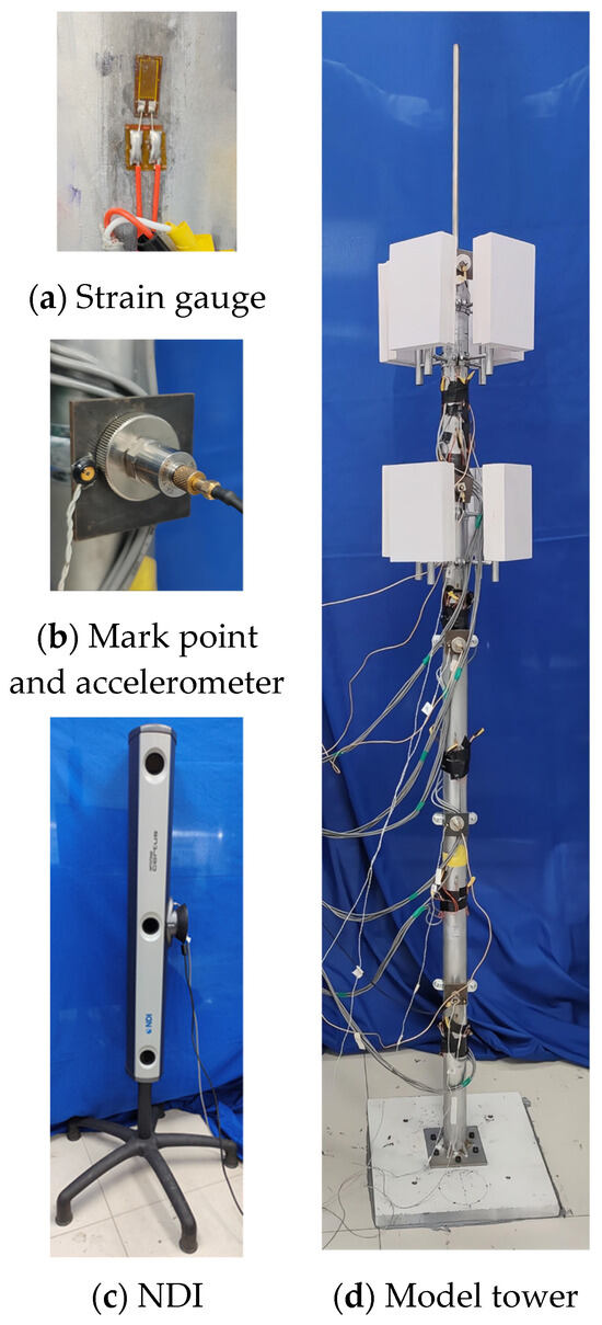
Figure 10.
Experimental models and sensors.
Table 6.
Sensor layout.
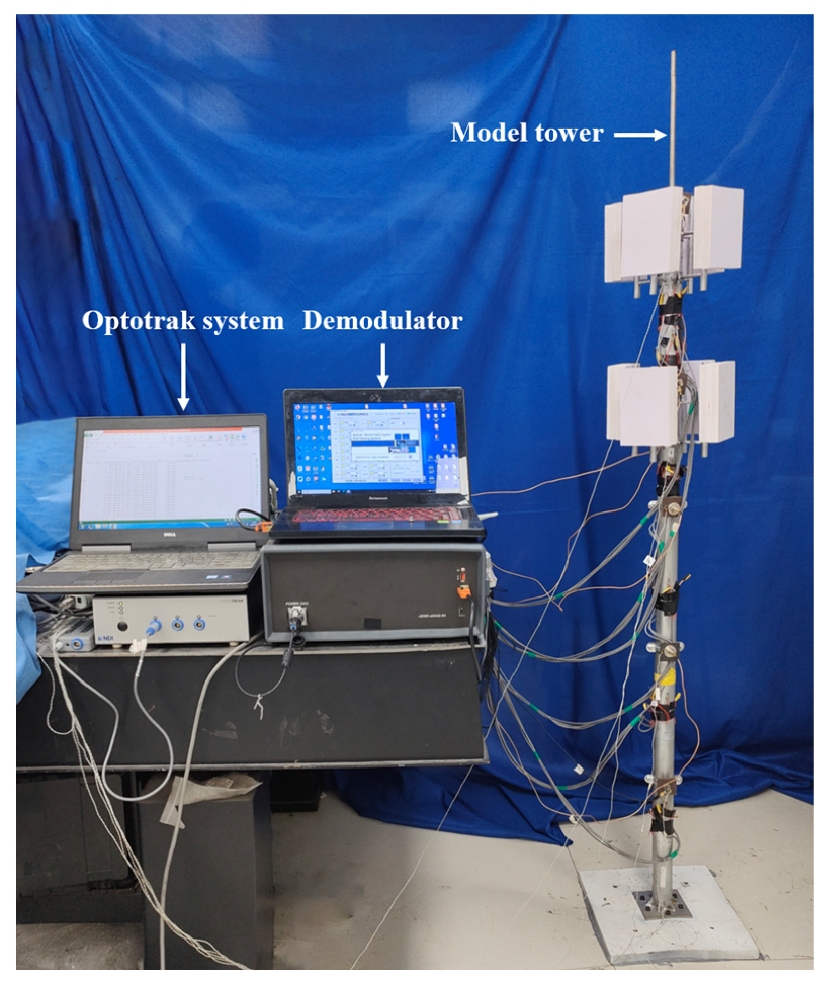
The experimental loading method uses the manual pushing method and percussion method. Pseudo-static force and two sudden loads are applied along the horizontal direction to the top of the model, resulting in pseudo-static displacement and high-frequency displacement of the model. The collected signals of accelerometers and strain gauges are demodulated using a self-developed photoelectric synchronous demodulator. The signals of NDI are collected with the Optotrak system developed by Northern Digital Inc. The experimental platform is shown in Figure 11, and the data collection time is 20 s.

Figure 11.
Experimental platform.
4.2. Comparison of Reconstructed Displacements
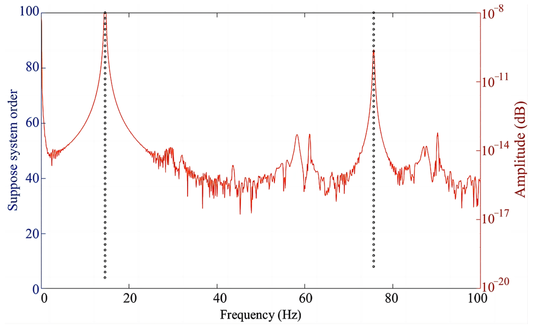
The stability plot and spectral curve of the measured strain and acceleration response time histories extracted using the SSI method are given in Figure 12. The symbols in the figure represent the same meaning as in Figure 4.
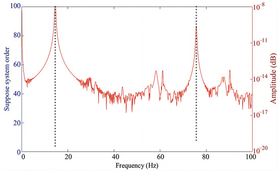
Figure 12.
Stability plot and spectral curve (model experiment).
The first two orders of the model frequency comparison are shown in Table 7. Although the error of the analytical results based on the model experiment increases compared with the numerical simulation results, the maximum is only 2.43% within 5%. It is also noted that the modal agreement between the experimental and numerical models is high within the error range. Accessory structures and connecting cables in the experimental model have less influence on the model modes.
Table 7.
Comparison of the first two-order frequencies (model experiment).
Strain modal superposition and Kalman filtering were performed on the experimental data to obtain the strain-derived and fused displacements, respectively. Then, the obtained displacement sampling rate was reduced to 300 Hz by resampling to compare with the measured displacement of NDI, as shown in Figure 13. It can be noted that the pseudo-static displacements restored by both methods almost completely coincide. This is because compared with acceleration, strain contains more low-frequency displacement information, so the difference in effectiveness between the two methods under pseudo-static loading is not significant. However, observing the localized zoomed-in plots of the high-frequency displacements from 9.7 to 10.0 s reveals that the accuracy of the strain-derived displacements is reduced. The data fusion displacement is closer to the measured displacement, indicating that acceleration contains more high-frequency displacement information, and the multi-source data fusion algorithm is more suitable for reconstructing high-frequency displacement.
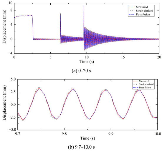
Figure 13.
Dynamic displacement reconstruction using different methods (model experiment).
4.3. Parametric Analysis
Since the experimentally collected data already contain natural noise, there is no need to add artificial noise to the data, and the effect of the SNR on the proposed algorithm will not be analyzed. In the following, only the effect of two parameters, the sampling ratio (SR) and distance ratio (DR), on the reconstruction accuracy of the algorithm are investigated. The designed working conditions are given in Table 8.
Table 8.
Working condition design (model experiment).
The effect of the SR on the reconstructed displacement reconstruction was first investigated. The acceleration sampling rate is still 1200 Hz, and the SRs are set to 4, 10, 20, and 40, respectively. Figure 14 shows the time-history plot of the reconstructed displacements versus the measured displacements at SR = 40. Compared with Figure 13, the reconstruction error of the reconstructed displacements increases. The high-frequency reconstructed displacements have a larger error and reduced accuracy compared with the pseudo-static reconstructed displacements. This is because the pseudo-static displacements vary at a low frequency and the displacements are well restored by the low-frequency strain response alone. In contrast, high-frequency displacement reconstruction relies on both acceleration and strain responses, with acceleration contributing significantly more. In the case of a high sampling rate ratio, the slowly changing pseudo-static displacement can be reconstructed with only a small amount of strain data. The reconstruction error of high-frequency displacements becomes larger due to the lack of a large amount of strain data to guide the displacement correction process. However, the reconstruction displacement error is only 3.01% at SR = 40, which shows that the proposed algorithm can adapt well to the large sampling rate difference among sensors.
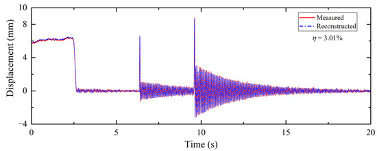
Figure 14.
Comparison of model experimental displacement reconstruction (SR = 40).
Table 9 shows η under different sampling ratios. The reconstructed displacement error increases with increasing sampling ratio, which is in accordance with the numerical simulations. However, even if the SR reaches 40, η is only 3.01%, proving that the proposed algorithm is suitable for high sampling ratios.
Table 9.
η under different SRs (model experiment).
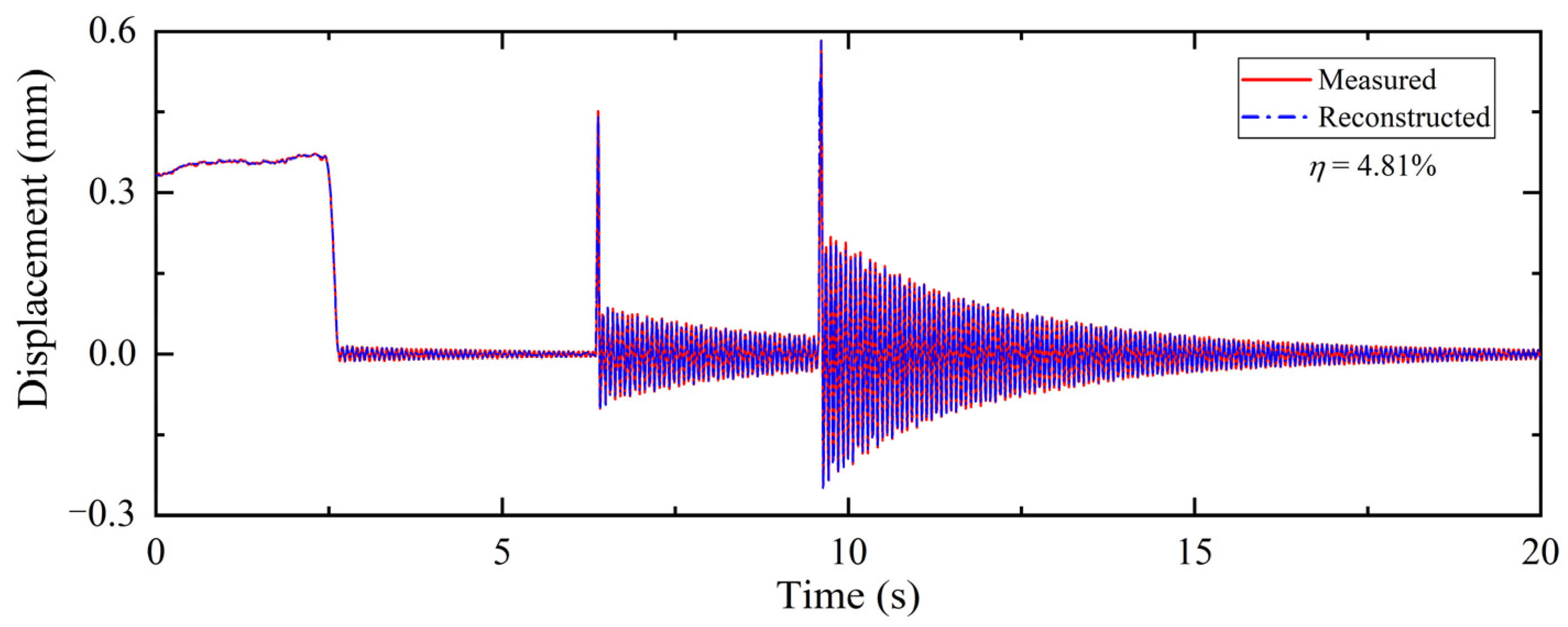
The influence of the distance ratio (DR) will be analyzed in the following, with the experimental loading method remaining unchanged. Using NDI to measure displacement can achieve synchronous real-time measurement of all mark points during the experimental process, avoiding artificial loading errors caused by multiple experiments. Mark points were set at 0.3, 0.6, 0.9, 1.2, and 1.5 m. Figure 15 shows the reconstructed displacement plot at DR = 0.2. It can be observed that the overall precision of the reconstructed displacements decreases, and the error of the high-frequency reconstructed displacements is larger. The reason is that the reconstructed point is near the bottom of the tower, which is more affected by the boundary conditions and more difficult to measure. The accuracy of low-frequency displacement reconstruction mainly depends on the single observation of strain, while high-frequency displacement reconstruction relies on both acceleration and strain data. Therefore, when the signal-to-noise ratio of the data is low, the high-frequency reconstruction displacement is more affected by the environment and the error is also greater. Although the accuracy of displacement reconstruction is affected by measured points, the maximum η is only 4.81%, proving that the fusion algorithm can well restore the displacement of the cantilever structure near the bottom.

Figure 15.
Comparison of model experimental displacement reconstruction (DR = 0.2).
Table 10 shows η under different DRs. It can be observed that the reconstructed displacement error of measurement points at 0.3, 0.6, and 0.9 m decreases as the distance from the measured point to the fixed end increases. However, the error slightly increases at 1.2 and 1.5 m, as the two measured points are located at the equipment layer. The accessory structure of the equipment layer affects the installation and measurement accuracy of the sensors, leading to an increase in the error of reconstruction displacement. Although the error slightly increases due to the influence of the equipment layer, the displacement error of the two points in the device layer still follows the rule of decreasing with increasing distance between the measured point and the fixed end, proving that the proposed displacement reconstruction method is not only available for simple cantilever structures but also has good applicability for complex structures.
Table 10.
η under different DRs (model experiment).
5. Conclusions
Monopole communication towers have high flexibility, and their slenderness ratio even exceeds that of typical high-rise structures. Excessive deformation is the main cause of damage to monopole communication towers, and dynamic displacement can be used as a key indicator to evaluate structural deformation. Therefore, this article proposes a dynamic displacement reconstruction algorithm for monopole communication towers based on multi-source data. First, the SSI method is used to obtain the strain displacements. Then, the strain displacement is calculated based on the strain-mode superposition methodology. After that, the low-sampling-rate strain responses and high-sampling-rate acceleration responses were inputted into the multi-rate Kalman filter algorithm to reconstruct the high-precision dynamic displacements. Finally, the validity of the proposed algorithm was verified using numerical simulations, model experiments, and parameter analysis. The conclusions are as follows:
- (1)
- The SSI method can precisely acquire the strain mode of the structure, thereby ensuring the accuracy of the observed displacements. The maximum error of the extracted vibration mode in the numerical simulation is 0.74%, while the maximum error in experiments is only 2.43%.
- (2)
- The proposed algorithm is applicable to the case of large differences in strain and acceleration sampling rates. In the numerical simulation, when SR = 100, η is only 2.28%. In the model experiment, when SR = 40, η is only 3.01%. This shows that the method can handle multi-rate data well.
- (3)
- The monopole communication tower is a cantilever-type structure. The theoretical displacement response at the fixed endpoints of the cantilever structure is zero. Thus, the closer the measurement point is to the bottom, the lower the precision of the reconstructed dynamic displacement. However, when DR = 0.2, the error of the numerical simulation is 2.46%, and the experimental value is 4.81%. Model experiments further show that the algorithm is well-suited for reconstructing displacements both at structural boundary locations and in complex environments.
- (4)
- The proposed algorithm has favorable noise resistance. In the numerical model, when adding noise with SNR = 5 dB to the strain and acceleration responses, respectively, η is only 5.53%. Processing experimental data containing natural noise, the results show that the algorithm can be successfully applied to the reconstruction of dynamic displacements of real structures.
The proposed multi-source data fusion algorithm based on strain responses and acceleration responses can fully utilize different types of data. The monopole tower model experiment has shown that this algorithm is not only suitable for simple cantilever-type structures but also for complex structures close to reality. It has great potential in the field of monopole tower monitoring in the future. Considering that the currently proposed method has only been validated using indoor experiments, the next study will be applied to the displacement reconstruction of actual monopole communication towers.
Author Contributions
Conceptualization, X.J. and L.R.; methodology, Q.Z. and X.F.; software, X.J. and Q.Z.; validation, X.J. and H.L.; formal analysis, X.J.; resources, L.R.; data curation, X.J. and H.L.; writing—original draft preparation, X.J.; writing—review and editing, X.F.; supervision, L.R. and X.F. All authors have read and agreed to the published version of the manuscript.
Funding
This research received no funding.
Data Availability Statement
The data presented in this study are available on request from the corresponding author.
Acknowledgments
The authors express their thanks to the people who have provided assistance with this work and acknowledge the valuable suggestions from peer reviewers.
Conflicts of Interest
The authors declare no conflict of interest.
References
- Carril, C.F.; Isyumov, N.; Brasil, R.M.L.R. Experimental study of the wind forces on rectangular latticed communication towers with antennas. J. Wind Eng. Ind. Aerod. 2003, 91, 1007–1022. [Google Scholar] [CrossRef]
- Fernández Lorenzo, I.; Clavelo Elena, B.; Martín Rodríguez, P.; Elena Parnás, V.B. Dynamic analysis of self-supported tower under hurricane wind conditions. J. Wind Eng. Ind. Aerod. 2020, 197, 104078. [Google Scholar] [CrossRef]
- Antunes, P.; Travanca, R.; Varum, H.; André, P. Dynamic monitoring and numerical modelling of communication towers with FBG based accelerometers. J. Constr. Steel Res. 2012, 74, 58–62. [Google Scholar] [CrossRef]
- Fu, X.; Wang, J.; Li, H.; Li, J.; Yang, L. Full-scale test and its numerical simulation of a transmission tower under extreme wind loads. J. Wind Eng. Ind. Aerod. 2019, 190, 119–133. [Google Scholar] [CrossRef]
- Del Coz Díaz, J.J.; García Nieto, P.J.; Lozano Martínez-Luengas, A.; Suárez Sierra, J.L. A study of the collapse of a WWII communications antenna using numerical simulations based on design of experiments by FEM. Eng. Struct. 2010, 32, 1792–1800. [Google Scholar] [CrossRef]
- Mulherin, N.D. Atmospheric icing and communication tower failure in the United States. Cold Reg. Sci. Technol. 1998, 27, 91–104. [Google Scholar] [CrossRef]
- Otunniyi, I.O.; Oloruntoba, D.T.; Seidu, S.O. Metallurgical analysis of the collapse of a telecommunication tower: Service life versus capital costs tradeoffs. Eng. Fail. Anal. 2018, 83, 125–130. [Google Scholar] [CrossRef]
- Nico, G.; Prezioso, G.; Masci, O.; Artese, S. Dynamic Modal Identification of Telecommunication Towers Using Ground Based Radar Interferometry. Remote Sens. 2020, 12, 1211. [Google Scholar] [CrossRef]
- Breuer, P.; Chmielewski, T.; Górski, P.; Konopka, E.; Tarczyński, L. The Stuttgart TV Tower—displacement of the top caused by the effects of sun and wind. Eng. Struct. 2008, 30, 2771–2781. [Google Scholar] [CrossRef]
- Xiao, Z.; Liang, J.; Yu, D.; Liu, J. Rapid three-dimension optical deformation measurement for transmission tower with different loads. Opt. Lasers Eng. 2010, 48, 869–876. [Google Scholar] [CrossRef]
- He, W.; Ge, S.S. Vibration Control of a Nonuniform Wind Turbine Tower via Disturbance Observer. IEEE/ASME T. Mech. 2015, 20, 237–244. [Google Scholar] [CrossRef]
- Celebi, M. GPS in dynamic monitoring of long-period structures. Soil Dyn. Earthq. Eng. 2000, 20, 477–483. [Google Scholar] [CrossRef]
- Moschas, F.; Stiros, S. High accuracy measurement of deflections of an electricity transmission line tower. Eng. Struct. 2014, 80, 418–425. [Google Scholar] [CrossRef]
- Lee, J.; Kim, H. Feasibility of in situ blade deflection monitoring of a wind turbine using a laser displacement sensor within the tower. Smart Mater. Struct. 2013, 22, 27002. [Google Scholar] [CrossRef]
- Lee, H.S.; Hong, Y.H.; Park, H.W. Design of an FIR filter for the displacement reconstruction using measured acceleration in low-frequency dominant structures. Int. J. Numer. Meth. Engng. 2010, 82, 403–434. [Google Scholar] [CrossRef]
- Cheng, Y.; Zhang, L.; Jiang, M.; Sui, Q. Strain/Displacement Field Reconstruction and Load Identification of High-Speed Train Load-Bearing Structure Based on Linear Superposition Method. IEEE T. Instrum. Meas. 2022, 71, 7003408. [Google Scholar] [CrossRef]
- Chen, K.; He, D.; Zhao, Y.; Bao, H.; Du, J. A Unified Full-Field Deformation Measurement Method for Beam-Like Structure. IEEE T. Instrum. Meas. 2022, 71, 1001110. [Google Scholar] [CrossRef]
- Hong, Y.H.; Kim, H.; Lee, H.S. Reconstruction of dynamic displacement and velocity from measured accelerations using the variational statement of an inverse problem. J. Sound Vib. 2010, 329, 4980–5003. [Google Scholar] [CrossRef]
- Popović, J.; Pandžić, J.; Pejić, M.; Vranić, P.; Milovanović, B.; Martinenko, A. Quantifying tall structure tilting trend through TLS-based 3D parametric modelling. Measurement 2022, 188, 110533. [Google Scholar] [CrossRef]
- Bang, H.; Kim, H.; Lee, K. Measurement of strain and bending deflection of a wind turbine tower using arrayed FBG sensors. Int. J. Precis. Eng. Man. 2012, 13, 2121–2126. [Google Scholar] [CrossRef]
- Li, M.; Kefal, A.; Oterkus, E.; Oterkus, S. Structural health monitoring of an offshore wind turbine tower using iFEM methodology. Ocean Eng. 2020, 204, 107291. [Google Scholar] [CrossRef]
- Liu, F.; Gao, S.; Chang, S. Displacement estimation from measured acceleration for fixed offshore structures. Appl. Ocean Res. 2021, 113, 102741. [Google Scholar] [CrossRef]
- Wu, B.; Tong, L.; Chen, Y. Revised Improved DINSAR Algorithm for Monitoring the Inclination Displacement of Top Position of Electric Power Transmission Tower. IEEE Geosci. Remote S. 2018, 15, 877–881. [Google Scholar] [CrossRef]
- Ma, Z.; Chung, J.; Liu, P.; Sohn, H. Bridge displacement estimation by fusing accelerometer and strain gauge measurements. Struct. Control Health Monit. 2021, 28, e2733. [Google Scholar] [CrossRef]
- Kim, K.; Kim, J.; Sohn, H. Development and full-scale dynamic test of a combined system of heterogeneous laser sensors for structural displacement measurement. Smart Mater. Struct. 2016, 25, 065015. [Google Scholar] [CrossRef]
- He, J.; Zhang, X.; Xu, B. KF-Based Multiscale Response Reconstruction under Unknown Inputs with Data Fusion of Multitype Observations. J. Aerosp. Eng. 2019, 32, 04019038. [Google Scholar] [CrossRef]
- Bock, Y.; Melgar, D.; Crowell, B.W. Real-Time Strong-Motion Broadband Displacements from Collocated GPS and Accelerometers. B. Seismol. Soc. Am. 2011, 101, 2904–2925. [Google Scholar] [CrossRef]
- Wang, Y.; Dai, K.; Xu, Y.; Zhu, W.; Lu, W.; Shi, Y.; Mei, C.; Xue, S.; Faulkner, K. Field Testing of Wind Turbine Towers with Contact and Noncontact Vibration Measurement Methods. J. Perform. Constr. Facil. 2020, 34, 04019094. [Google Scholar] [CrossRef]
- Park, J.; Sim, S.; Jung, H. Displacement Estimation Using Multimetric Data Fusion. IEEE/ASME T. Mech. 2013, 18, 1675–1682. [Google Scholar] [CrossRef]
- Zhu, H.; Gao, K.; Xia, Y.; Gao, F.; Weng, S.; Sun, Y.; Hu, Q. Multi-rate data fusion for dynamic displacement measurement of beam-like supertall structures using acceleration and strain sensors. Struct. Health Monit. 2020, 19, 520–536. [Google Scholar] [CrossRef]
- He, W.; Liu, P.; Cheng, H.; Li, Z.; Bu, J. Displacement reconstruction of beams subjected to moving load using data fusion of acceleration and strain response. Eng. Struct. 2022, 268, 114693. [Google Scholar] [CrossRef]
- Sun, L.; Li, Y.; Zhang, W. Experimental Study on Continuous Bridge-Deflection Estimation through Inclination and Strain. J. Bridge Eng. 2020, 25, 04020020. [Google Scholar] [CrossRef]
- Khodabandeloo, B.; Melvin, D.; Jo, H. Model-Based Heterogeneous Data Fusion for Reliable Force Estimation in Dynamic Structures under Uncertainties. Sensors 2017, 17, 2656. [Google Scholar] [CrossRef] [PubMed]
- Moor, B.L.R.D.; Overschee, P.V. Subspace Identification for Linear Systems: Theory, Implementation, Applications, 1st ed.; Kluwer Academic Publishers: New York, NY, USA, 1996; p. 254. [Google Scholar]
- Khaleghi, B.; Khamis, A.; Karray, F.O.; Razavi, S.N. Multisensor data fusion: A review of the state-of-the-art. Inform. Fusion 2013, 14, 28–44. [Google Scholar] [CrossRef]
- Yang, Y.; Jung, H.K.; Dorn, C.; Park, G.; Farrar, C.; Mascareñas, D. Estimation of full-field dynamic strains from digital video measurements of output-only beam structures by video motion processing and modal superposition. Struct. Control Health Moni. 2019, 26, e2408. [Google Scholar] [CrossRef]
- Hong, Y.H.; Lee, S.G.; Lee, H.S. Design of the FEM-FIR filter for displacement reconstruction using accelerations and displacements measured at different sampling rates. Mech. Syst. Signal Pract. 2013, 38, 460–481. [Google Scholar] [CrossRef]
- Thomas, J.; Gurusamy, S.; Rajanna, T.R.; Asokan, S. Structural Shape Estimation by Mode Shapes Using Fiber Bragg Grating Sensors: A Genetic Algorithm Approach. IEEE Sens. J. 2020, 20, 2945–2952. [Google Scholar] [CrossRef]
- Guo, X.; Li, C.; Luo, Z.; Cao, D. Modal Parameter Identification of Structures Using Reconstructed Displacements and Stochastic Subspace Identification. Appl. Sci. 2021, 11, 11432. [Google Scholar] [CrossRef]


Disclaimer/Publisher’s Note: The statements, opinions and data contained in all publications are solely those of the individual author(s) and contributor(s) and not of MDPI and/or the editor(s). MDPI and/or the editor(s) disclaim responsibility for any injury to people or property resulting from any ideas, methods, instructions or products referred to in the content. |
© 2023 by the authors. Licensee MDPI, Basel, Switzerland. This article is an open access article distributed under the terms and conditions of the Creative Commons Attribution (CC BY) license (https://creativecommons.org/licenses/by/4.0/).