Article

Machine Learning-Aided Prediction of Post-Fire Shear Resistance Reduction of Q690 HSS Plate Girders

1
School of Management Science and Real Estate, Chongqing University, Chongqing 400045, China
2
School of Civil Engineering, Chongqing University, Chongqing 400045, China
*
Author to whom correspondence should be addressed.
Buildings 2022, 12(9), 1481; https://doi.org/10.3390/buildings12091481
Submission received: 31 August 2022 / Revised: 14 September 2022 / Accepted: 14 September 2022 / Published: 17 September 2022
(This article belongs to the Special Issue Recent Advances in Constructional Steel Research)

Abstract

:
Fire has significant effects on the residual resistance of steel structures. It is necessary to accurately clarify its effects on Q690 HSS plate girders, which have been widely used. In this paper, the ultimate resistance and effective service resistance of Q690 HSS plate girders after a fire are obtained using material tests and finite element (FE) analysis including parametric studies, where the data of 210 models were collected. The effects of four key parameters (hw/tw ratio, a/hw ratio, exposure temperature and cooling method) on post-fire shear resistance reduction of Q690 HSS plate girders are roughly investigated by individual conditional expectation (ICE), showing exposure temperature is the most important factor. The popular algorithms of machine learning (ML), namely artificial neural network (ANN) and support vector regression (SVR) algorithms, are utilized in model training to predict the reduction factors of both ultimate resistance and effective service resistance. Finally, the results indicate that the prediction using ML shows much better performance than that with traditional ordinary least squares (OLS) regression, and SVR with genetic algorithm (GA) provides the highest prediction accuracy. The results of this paper show the superiority of machine learning for solving prediction problems of steel structures, compared with conventional methods such as linear regression.

1. Introduction

High-strength steel (HSS) with a yield strength of higher than 460 MPa has been widely used in high-rise buildings and long-span structures. Compared with mild steel, HSS possesses higher strength properties, which reduces the steel consumption of structures and the difficulty of welding.
However, it is worth noting that the elastic modulus of HSS is similar to that of mild steel. Therefore, the use of HSS could not bring beneficial effects on the buckling resistance, which is mainly influenced by the dimensions of the component and the elastic modulus of the material. When the steel component exhibits stable buckling, the load on the steel component could still increase after buckling because of post-buckling resistance. The plate structures usually have noteworthy post-buckling resistance [1,2]. The plate girder (PG) investigated in this study is a welded I-section girder with a large web-height-to-thickness ratio (see Figure 1). In order to improve the buckling resistant capacity of the web, the steel plate girder is usually strengthened by transverse stiffeners. Because of the embedment effects from the flange and transverse stiffener on the web, there is post–buckling capacity in the plate girder. In that case, when the steel plate girder is subjected to shear load, the web first exhibits the local buckling. After that, the shear load could be made resistant stably using a plate girder, where no decrease in resistant stiffness is observed. Then, the steel plate girder develops post-buckling resistant capacity. Many scholars have studied the post-buckling performance of steel plate girders. Hassanein studied the ultimate resistance of stainless steel plate girders through finite element analysis [3], where the design equations in different codes were validated based on the numerical results. Alinia et al. [4] performed a numerical investigation on the stress evolution in the web of plate girders, which clarified the transition from the buckling state to the ultimate state. Considering the post-buckling resistance of the plate girder, the strength properties of the steel perform noteworthy effects on the resistant properties of the plate girder, which means the outstanding strength properties of HSS could be fully utilized. Thus, HSS has been a promising material for plate girders [5,6,7]. Choi et al. [5] studied the shear behavior of web panels in HSB800 plate girders, which suggested a predictive method for the ultimate shear resistance. Xiao et al. [8] clarified the effect of the nonlinear properties of Q690 HSS on the shear capacity of a plate girder. Azizinamini et al. [9] conducted the experiment on the plate girder consisting of mild steel and HSS, which provided the test results for the tension field action of the web during the post-buckling segment. Despite all this research, the post-buckling resistance of the HSS plate girder still needs to be studied thoroughly. Some current investigations ignored the beneficial effects of the strain hardening properties of the structural steel. Because of the strain hardening properties of structural steel, the stress of the web during the post-buckling segment could increase gradually, which brought beneficial effects on the resistance of the plate girder. When there was a yield plateau in the stress–strain curve, the beneficial effects of strain hardening properties were reduced. Nonlinear stress-strain properties of the structural steel perform noteworthy effects on the stress distribution of the plate girder, which influences the resistant properties. The above issue should be answered to clarify the resistant properties of the plate girder comprehensively.
Fire is considered to be one of the severe hazards that can destroy buildings [10,11,12,13,14,15,16], reducing the service life of constructions [17]. For steel structures, the high thermal conductivity and low specific heat make the case more dangerous. The rapid rise in temperature significantly changes the microstructures of the steel [18], leading to a significant reduction in the elastic modulus and strength properties of structural steel [19]. When the steel structure experiences fire without collapse and significant residual deformation, it is necessary to accurately evaluate the residual resistant performance of the steel structure. Once given the residual resistance of the steel structure after a fire, a decision could be made about the subsequent application of the post-fire steel structure, such as direct use, use after repair or demolishing. As a result, it is necessary to clarify the residual mechanical properties of structural steel after a fire and to this end, many experimental studies have been conducted [20,21]. Li et al. [22] performed an experiment to clarify the effects of exposure temperature and cooling methods on the residual mechanical properties of Q690 HSS, where comprehensive predictive equations were suggested based on test results. Qiang et al. [23] studied the post-fire mechanical properties of S460 and S690 HSSs with cooling in air, where the reduction in strength properties was discussed. According to current studies, the exposure temperature has more obvious effects on the mechanical properties of HSS, compared with that of mild steel. Additionally, the reduction in the resistance of HSS structures after a fire might be larger than that of mild steel structures. Consequently, the resistant performance of HSS plate girders exposed to elevated temperatures should be investigated. The key parameters influencing the residual resistance of HSS plate girders after a fire may include the dimensions of the plate girder, exposure temperature and cooling method. It should be noted that the resistance of the plate girder was significantly influenced by the post-buckling behavior, where the load transfer mechanism changed. In general, it is difficult to suggest predictive equations with a clear physical meaning to clarify the effects of multiple variables, considering that there was a coupling effect between different variables.
Recently, machine learning (ML) has been a hot topic of interest for researchers [24]. It has a strong ability to capture complicated relations among input and output data in handling complex nonlinear structural analysis [24,25,26]. A large number of studies have demonstrated that ML can be an accurate and efficient alternative approach to traditional techniques for damage detection (classification problems) and strength predictions (regression problems) in structural engineering [24,26]. Specifically, the ML approach is a great tool for analyzing the mechanical problems of steel structures, which is the case of this study. For example, two representative ML algorithms including support vector regression (SVR) and artificial neural network (ANN) could be used to predict the ultimate strength of concrete-filled cold-formed steel tubular (CFCFST) columns under concentric and eccentric loading [27]. ANN is also employed in the material modeling of steel when exposed to the high temperatures expected in fires [28]. In addition to ANN and SVR, other advanced ML algorithms (i.e., Extreme Gradient Boosting (XGBOOST), and Light Gradient Boosting Machine (LightGBM) could be good choices to forecast the shear strength in steel buildings accurately [29].
When solving regression problems, ANN and SVR models have mature algorithms and they are simple to use [30]. ANN imitates the structure and mechanism of the human brain, which is able to fit any relationship between input and output parameters, showing its great potential to predict and identify the results [31]. SVR represents an extension of SVM for regression problems, which is widely used for prediction in both linear and nonlinear regression analyses, for its relatively high generalization ability, even with limited samples [32].
Considering the complexity of the issue investigated in this study, ANN and SVR are proposed to improve the prediction of the residual resistance of Q690 HSS plate girders after a fire. The main body of this paper is structured as follows: Section 2 briefly introduces the process of data collection, containing material tests, finite element modeling, parametric studies and the basic algorithm of linear regression. The ML methodology is presented in Section 3, which also discusses hyperparameter optimization. Subsequently, Section 4 demonstrates the results of the predictive models for the ultimate resistance and effective service resistance reduction factors (TVu/20Vu ratio and TVe/20Ve ratio) and correlation analysis is shown. Section 5 presents the discussions and future works.

2. Data Collection

2.1. Material Tests

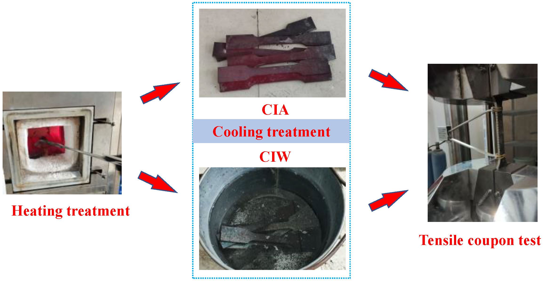
The material tests were conducted to clarify the residual mechanical properties of Q690 HSS after exposure to elevated temperature. The chemical composition of Q690 HSS studied in this research is listed in Table 1. The mechanical test specimens were cut from one Q690 HSS sheet. The dimensions of the test specimen were determined according to the requirements in GB/T 228.1-2010 [33], as shown in Figure 2. The test process in this study was the same as that in Ref. [20], as presented in Figure 3. Firstly, the MXQ1400-30 temperature-controlled electric furnace was used to heat the Q690 HSS specimen for simulating the fire load, where the exposure temperatures including 300/400/500/600/700/800/900 °C were considered. Then, two different cooling methods were applied, respectively, namely cooling in air (CIA) and cooling in water (CIW) [20,21,22,23]. For each cooling method and exposure temperature combination, three test specimens were prepared. The test specimen without heating and cooling treatment was also involved as the benchmark. Finally, the tensile coupon test was carried out after cooling treatment, where the loading rate was controlled to be 1 mm/min, within the required range of GB/T 228.1-2010 [33]. An extensometer was used to record the deformation of the test segment in the specimen. The load data was read from the testing system and the loading will be terminated when the fracture of the test specimen was observed.
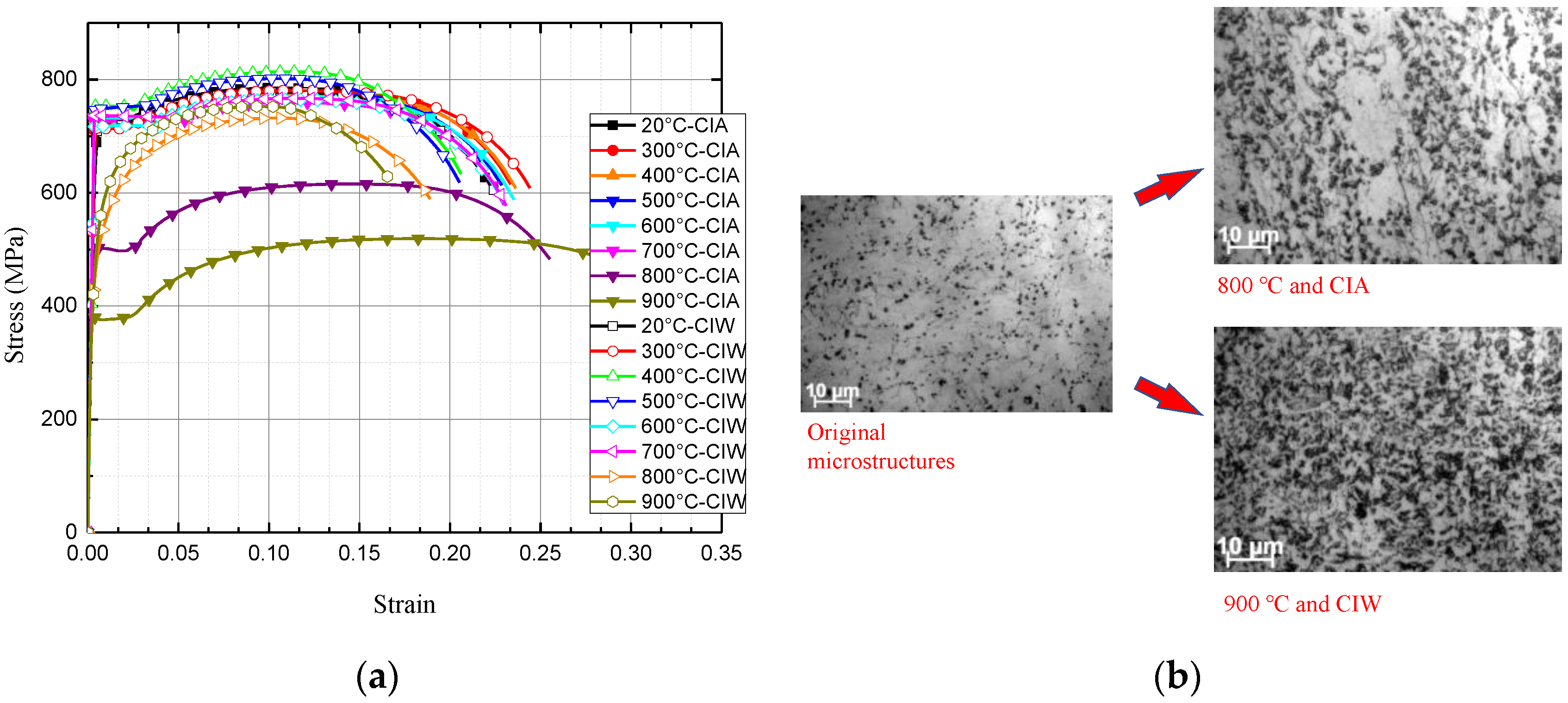
Based on the load-displacement data, the stress-strain curves of the test specimens were obtained, as shown in Figure 4a. Test results indicated that when the exposure temperature was lower than 700 °C, the residual stress-strain curves were almost identical to the ones without fire. When the exposure temperature was higher than 700 °C, the reductions in stress-strain properties of Q690 HSS were clearly seen. In that case, the effects of fire on the residual resistance of the Q690 HSS plate girder should be given attention. Specifically, when the exposure temperature ranged from 700 °C to 900 °C, the reduction in strength properties for CIW specimens was clearly lower than that of specimens with CIA, which was caused by the quenching effect. A similar phenomenon was also observed in Refs [21,34]. However, the current investigations on the post-fire mechanical properties of Q690 HSS mainly focused on the stress-strain properties. There has been limited research considering the microstructures of the Q690 HSS after exposure to elevated temperatures [20,35,36]. To reveal the reason for the differences in the stress-strain properties, it was meant to clarify the stress-strain properties. In this study, the microstructures of the Q690 HSS with different cooling methods and exposure temperatures were discussed. The microstructures of the test specimens were observed after the tensile coupon test for further analysis, as presented in shown in Figure 4b. For the Q690 HSS at room temperature (benchmark), there were ferrite (white area) and pearlite (black dot), where the area proportion of ferrite was obviously higher than that of pearlite. For Q690 HSS after 800 °C heating and CIA cooling, compared to the benchmark specimen, the area proportion of granular pearlite increased while the size of ferrite seemed to be larger. The above changes in microstructures led to a decrease in strength and an increase in ductility, which agreed with the tendency of stress-strain curves in Figure 4a. For Q690 HSS with 900 °C exposure temperature and CIW, cementite was widely dispersed in the range of ferrite, which brought beneficial and adverse effects to the strength and ductile properties, respectively. This characteristic in the microstructure might be the reason for the disappearance of the yield plateau, as seen in curves of 800 °C-CIW and 900 °C-CIW. For the Q690 HSS in this study, when exposure temperature was higher than 700 °C, exposure temperature was higher than the austenitizing temperature of Q690 HSS, where a clear transformation of the metallographic structure was observed. Differences in microstructures led to differences in mechanical properties. The austenitizing temperature of mild steel might be different from that of Q690 HSS, which might lead to different turning points.
Considering the test results above, in the following numerical analysis, the stress-strain properties of Q690 HSS with 25/700/800/900 °C exposure temperatures and CIW/CIA cooling methods would be introduced to study the residual resistance of the Q690 plate girder after a fire.

2.2. Finite Element (FE) Modeling

The finite element (FE) model of the Q690 HSS plate girder was established using ABAQUS software, as shown in Figure 5a. The S4R shell element was selected to simulate the steel plate in the Q690 HSS plate girder [5,6,7,37]. To simulate the welding, the “Tie” constraint was set to build a connection between the web (flange) and transverse stiffener. The true stress-strain relations of steel were calculated using averaged engineering stress-strain data (equations were introduced in Ref. [6]) in Section 2.1, later imported to ABAQUS. The true stress and strain equations are given in EN 1993-1-5:2006 [38]. Simply supported boundary condition was selected. The end sections of the plate girder model were coupled to the reference points. Then, the rotational and translational degrees of freedom of the reference points were restrained to simulate the simply supported boundary condition. The details about rotational and translational degrees of freedom of the reference points were introduced in Ref. [8]. Some lateral supports were introduced in the flange to avoid lateral–torsional buckling, which was used to simulate the constrained effect from beams and floor on the plate girder. It is worth noting that the initial imperfection was considered by introducing the first buckling mode obtained from the elastic buckling analysis, where the peak value of the initial imperfection was determined to be 1/100 of web height (hw), as recommended in section 9 of the AASHTO Bridge Welding Code [39]. The above peak value of the initial imperfection was also recommended in Refs. [3,40,41]. The convergence study was performed based on a typical model to determine the proper size of the element mesh. The results are shown in Figure 5b, where the error is (Vu,iVu,2)/Vu,2, in which Vu,i and Vu,2 denote the ultimate resistance of the plate girder whose element size is i and 2 mm, respectively. To balance the accuracy and calculation consumption, the element size was determined to be 20 mm, which meant the error would be below 2%. The accuracy of the above numerical modeling method had been validated by the experimental results of mild steel plate girders [7,8] and stainless steel plate girders [6] comprehensively. It is worth noting that the post-fire stress-strain properties of the Q690 HSS were similar to those of mild steel and stainless steel, such as the yield plateau, strain-hardening effect and so on. Hence, it is believed that the numerical modeling method validated by the experimental results on the mild steel and stainless-steel plate girders could be used to predict the resistant properties of the Q690 HSS plate girder after fire effectively. It is worth noting that the experimental and numerical investigations in this study were focused on the post-fire-resistant properties of the Q690 HSS plate girder, considering the effects of exposure temperature and cooling method.

2.3. Parametric Study

Based on the modeling technics introduced in Section 2.2, a parametric study was conducted involving 210 FE models. The material properties of Q690 HSS under different exposure temperature and cooling methods were identical to the test results reported in Section 2.1, where the reduction factors for the stress properties of steels have been listed in Table S1 in the Supplementary Materials. For all the models, web thickness is tw = 5 mm, and the flange width (bf) and thickness (tf) are 200 mm and 20 mm, respectively. The key parameters include the height-to-thickness ratio of web hw/tw (100/150/200/250/300), aspect ratio of web a/hw (0.5/0.75/1/1.25/1.5/2), exposure temperature (20/700/800/900 °C) and cooling method (CIA and CIW), where a is the spacing of transverse stiffeners, which are the applicable ranges of input parameters of the predictive model. Based on the experimental results introduced in Section 2.1, the effects of exposure temperature and cooling method on the post-fire mechanical properties of the Q690 HSS were ignorable, when the exposure temperature was lower than 700 °C. Hence, there was almost no difference in the resistant properties of the Q690 HSS plate girder after exposure to an elevated temperature below 700 °C. Therefore, the exposure temperatures below 700 °C were not included in the parameter study. The span of the place girder (L) could be calculated by L = 2a + 320 mm. The effects of tw on the resistant properties of plate girder are reflected in the hw/tw, which is recommended by many researchers [6,7,8,40,42]. Basically, the flanges of plate girder provide the bending moment resistance rather than the shear resistance, so the effects of the bf and tf on the shear-resistant properties of the plate girder are relatively small. Hence, the tw, bf and tf are not varied in this study. The geometry details of each model are introduced in Table S2 in the Supplementary Materials.
For all the FE models in this study, the flange plastic hinge mode was observed, which is the expected failure mode in the design code [43]. In this study, the ultimate resistance Vu corresponding to the peak point of the resistance curve and the effective service resistance Ve corresponding to the L/400 midspan displacement were selected to quantify the resistant properties of Q690 HSS plate girders with different cooling methods and exposure temperatures. Based on the requirement in GB 50017-2017 [44] for the deflection limit of the plate girder with different bearing functions and loading conditions, the deflection limit L/400 was selected. The Vu and Ve values of each model with different dimensions, exposure temperature and cooling methods are listed in Table S3–S5 in the Supplementary Materials.
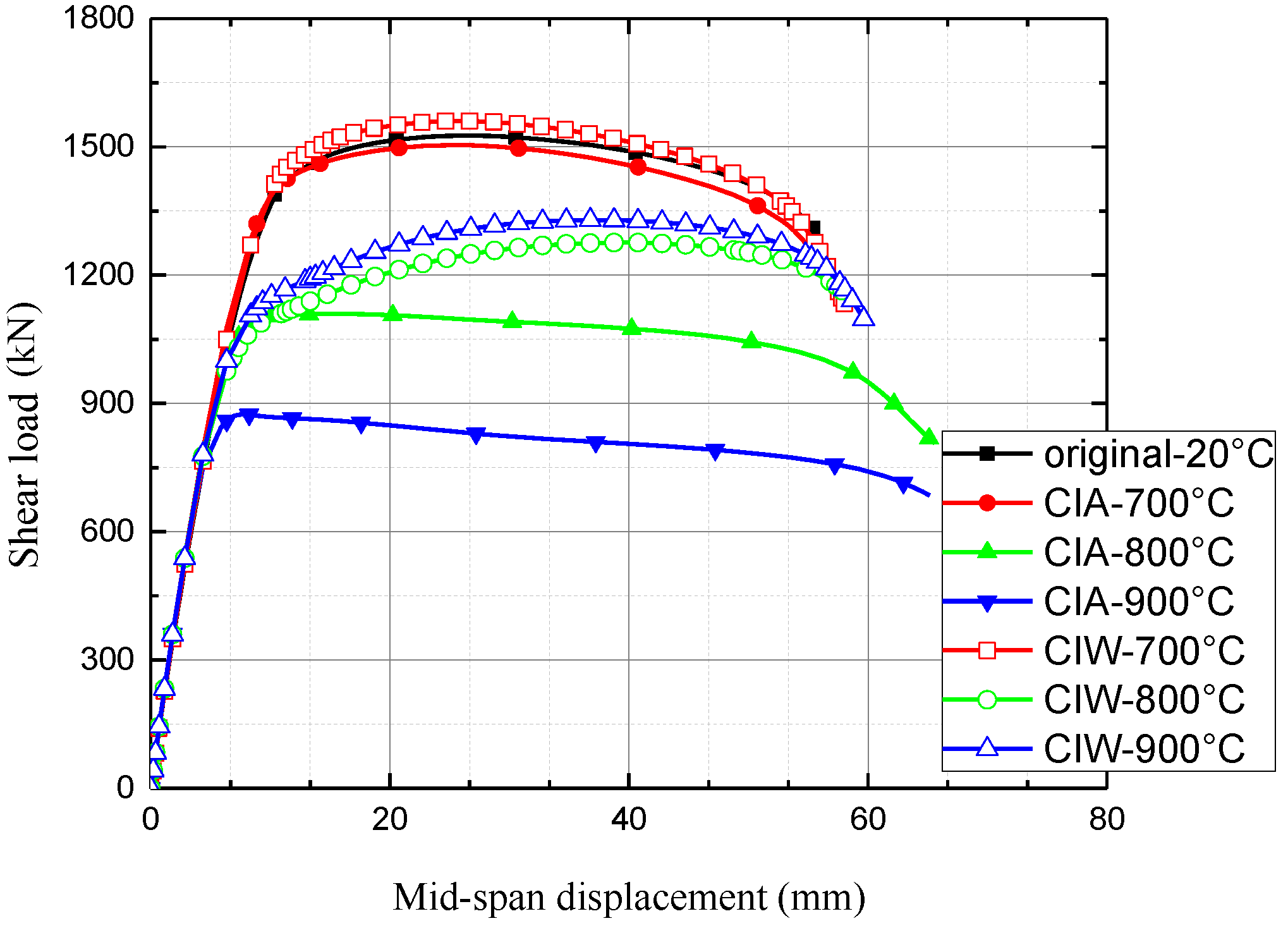
As for the load-midspan displacement curves, the typical model P-1-250 (which meant a/hw = 1 and hw/tw = 250) is selected to clarify the effects of exposure temperature and cooling method, as shown in Figure 6. When the CIA is applied, with increments in the exposure temperature, the resistant performance of Q690 HSS plate girders decreases, gradually. When the exposure temperature is 700 °C, the resistance curves are similar to that of the Q690 HSS plate girder at 20 °C. When the exposure temperatures are 800 and 900 °C, the resistant performance is clearly poorer than that of the Q690 HSS plate girder with 20 °C, along with the change in the nonlinear tendency of curves. For the curve of the Q690 HSS plate girder at 20 °C, when the elastic segment is over, the noteworthy strengthening segment is observed. However, when the exposure temperatures are 800 and 900 °C, there is barely any such strengthening segment in the resistance curves of Q690 HSS plate girder hw/tw with CIA. When the elastic segment is over, the peak point is reached rapidly. When the CIW is performed, the resistance curve of the Q690 HSS plate girder exposed to 700 °C is similar to that of the Q690 HSS plate girder at 20 °C. When the exposure temperature increases from 700 °C to 800 °C or 900 °C, the resistance of the Q690 HSS plate girder decreases correspondingly. It should be noticed that the resistance of the Q690 HSS plate girder with exposure temperature of 900 °C and CIW is better than that of the Q690 HSS plate girder with exposure temperature of 800 °C and CIW. The above increment in resistant performance is caused by the quenching effects of the stress-strain properties mentioned in Section 2.1. Compared with Q690 HSS plate girders with CIA, the Q690 HSS plate girders with CIW always have higher resistance.
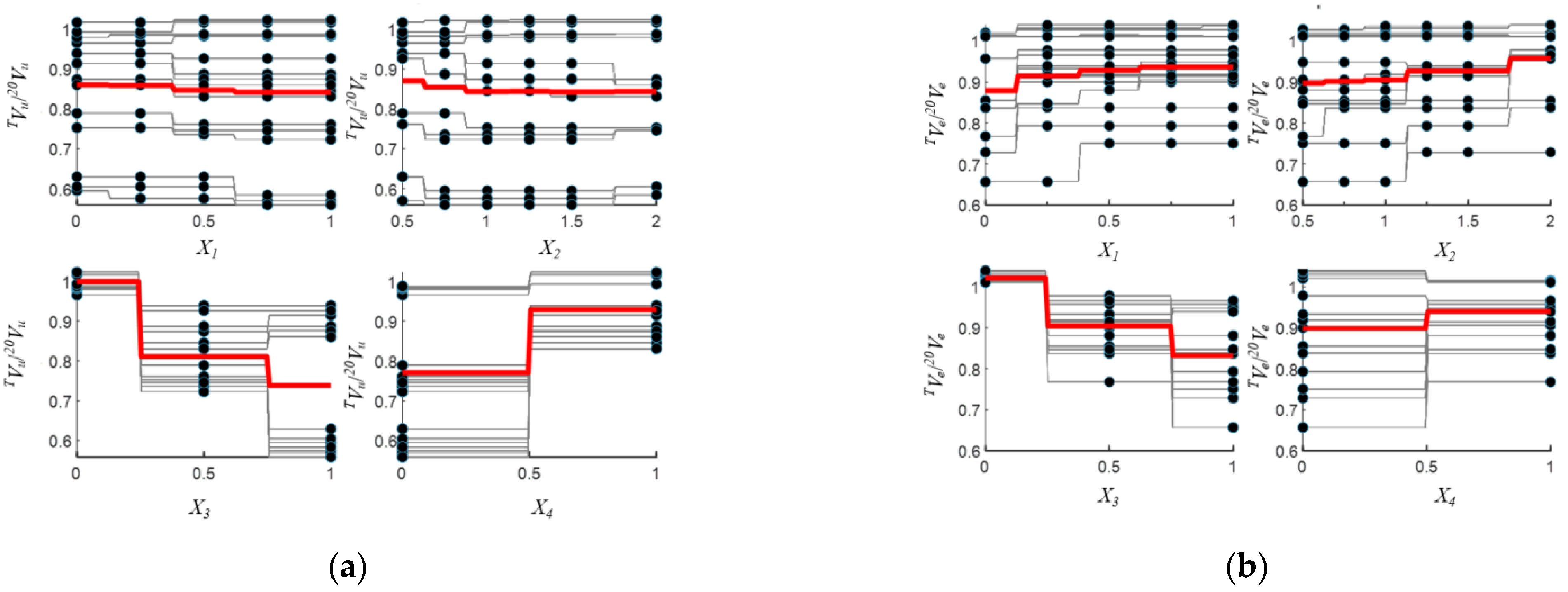
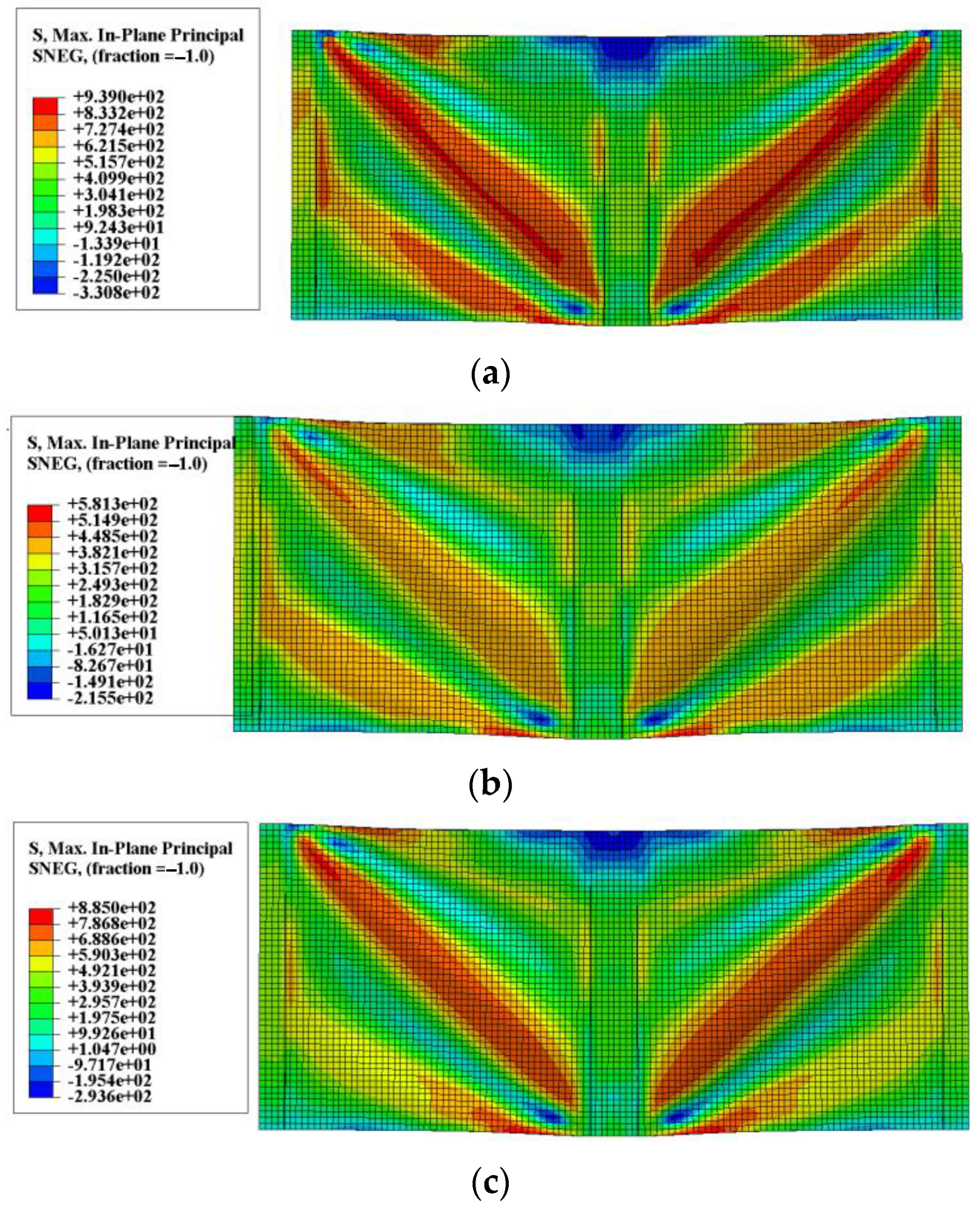
Generally, the effect of fire on the resistance of the plate girder could be quantified by the reduction factor, which is a great concern. Therefore, in this study, the effect of the key parameters on the post-fire resistance reduction factors for the ultimate resistance and effective service resistance (TVu/20Vu ratio and TVe/20Ve ratio) are studied, where TVu and TVe are the resistance after exposure to elevated temperature T, while 20Vu and 20Ve are the resistances under room temperature (20 °C). The correlation analysis is proposed by individual conditional expectation (ICE), which can be used to visualize or quantify the impact of every input variable on the output variable [45]. It shows how the output changes when one of the four input variables changes, while the other three variables remain unchanged. Each line represents one occasion of the impact on the TVu/20Vu or TVe/20Ve ratio of each Xi, and the red line is expected to reflect the average trend, where X1, X2, X3 and X4 represent the hw/tw ratio, a/hw ratio, exposure temperature and cooling method (0 denotes CIA while 1 denotes CIW), respectively. Figure 7 shows that both the TVu/20Vu ratio and the TVe/20Ve ratio are influenced by the four parameters. As can be seen, Figure 7a shows a trend towards a gradual decrease in the TVu/20Vu ratio with higher exposure temperature (X3). Although the cooling method (X4) has an obviously positive effect on TVu/20Vu ratio, which means the CIW method has a more beneficial effect than the CIA method. Additionally, the influence of hw/tw (X1) and a/hw (X2) on the TVu/20Vu ratio is complex, and almost no overall conclusion could be made. As for the TVe/20Ve ratio, Figure 7b proves that exposure temperature (X3) is the most significant factor with a negative effect, and the positive effect is seen between hw/tw (X1) and the TVe/20Ve ratio, as well as the a/hw (X2) and TVe/20Ve ratios. The impact of the cooling method (X4) on the TVe/20Ve ratio seems to be complicated, but overall, the reduction factor is higher for those using CIW, rather than CIA. The stress distributions and failure modes corresponding to the ultimate resistance of the plate girder model with different cooling methods and exposure temperatures are shown in Figure 8, where a/hw = 1 and hw/tw = 200. Local buckling is observed in the web while the plastic hinges occurred in the flange. Effects of the cooling method and exposure temperature on the failure mode are relatively small. However, the tension field of the web is changed after fire exposure.

2.4. Prediction of Resistance Reduction through Linear Regression

Regression analysis is a commonly-used method to model the simple relationship between the independent variables and dependent variables. Linear regression analysis researches the relationship by building a linear equation [46] and one of the most popular ways is the ordinary least squares (OLS). OLS regression fits a straight line, which satisfies the demand of minimizing the squared vertical distance from all observations to the regression line on the scatter plot [47]. As concluded in Section 2.3, the TVu/20Vu ratio and TVe/20Ve ratio are both highly influenced by the hw/tw ratio, a/hw ratio, exposure temperature and cooling method. Therefore, the equations for the simple linear regression are obtained below. Considering that the numerical analysis was focused on the variable scope in Section 2.3, the input parameters of the predictive model should be controlled within the above applicable ranges.
T V u / 20 V u = α 1 X 1 + α 2 X 2 + α 3 X 3 + α 4 X 4 + ε 1
T V e / 20 V e = β 1 X 1 + β 2 X 2 + β 3 X 3 + β 4 X 4 + ε 2
where TVu/20Vu ratio and TVe/20Ve ratio are the dependent variables, Xi represents the independent variables after pre-processing (the process of generation and normalization is illustrated in Section 3.1), αi (i = 1,2,3,4) and βi (j = 1,2,3,4) are the regression coefficients and εk (k = 1,2) is an error to account for the difference between predicted data and the true data. It is worth noting that the reduction factor is investigated in this manuscript, where the ultimate shear resistance of the Q690 plate girder without exposure to elevated temperature is considered to be the benchmark. Therefore, when the design standard could be used to predict the ultimate shear resistance of Q690 plate girder without exposure to elevated temperature accurately, the predictive model in this manuscript could be used to predict the ultimate shear resistance of Q690 plate girder after exposure to elevated temperature, which quantifies the reduction factor.
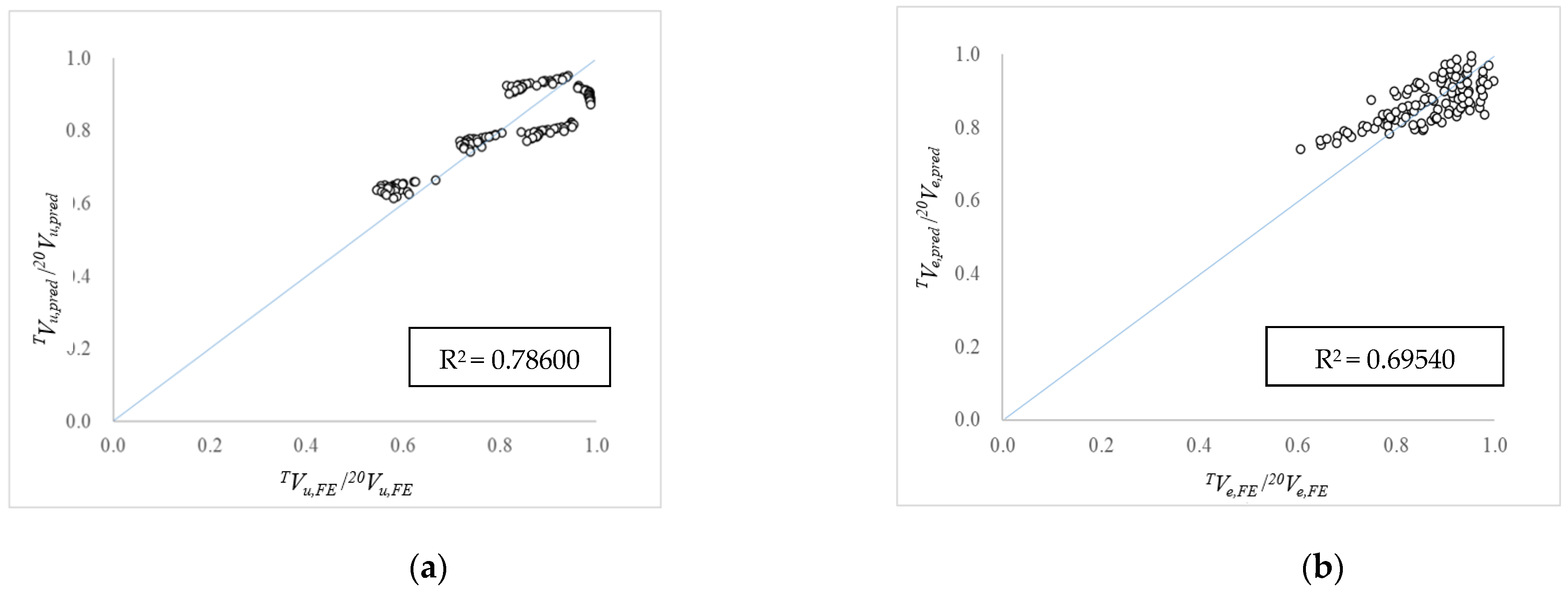
The results of the OLS regression analysis are presented in Figure 9 and the analysis of variance (ANOVA) is shown Table 2. Generally speaking, a model that maximizes the coefficient of determination (R2) is considered to be more accurate [46], so R2 serves as a vital statistical metric for comparison among all the methods in this study. R2 indicates the statistical relationships between the true value and the predicted value, and the formula is shown in Equation (3).
R 2 = 1 i = 1 n ( y i y ^ i ) 2 i = 1 n ( y i y ¯ ) 2
where, y ^ i and yi are the ith true and predicted values, respectively; y represents mean value of yi.
The R2 values of the linear regression model for the TVu/20Vu ratio and TVe/20Ve ratio are 0.7860 and 0.6954, respectively. The R2 values are not high enough for accurate prediction but it could be concluded that the considered parameters have a reasonable contribution to explaining the behavior of TVu/20Vu ratio and TVe/20Ve ratio, at least for this linear model. In Table 2, the statistical P-value for each parameter (independent variable) is listed, which could be used to measure whether the parameter is statistically significant to the dependent variable. Variables with a p-value lower than 0.1 (marked with “*”) are effective, and variables with a p-value lower than 0.01(marked with “***”) could be regarded as highly significant parameter [48]. Specifically, for the TVu/20Vu ratio, hw/tw and a/hw are effective, and the exposure temperature and cooling method are highly significant. For TVe/20Ve, all the parameters are highly significant. According to the coefficients (Coef), all independent variables have negative effects on TVu/20Vu ratio except the cooling method, while all have positive effects on TVe/20Ve ratio except exposure temperature. However, linear regression has some limitations in prediction accuracy. Thus, for a better prediction, the machine learning methods are introduced and applied in the following sections.

3. Machine Learning Methodology

3.1. Overall Introduction

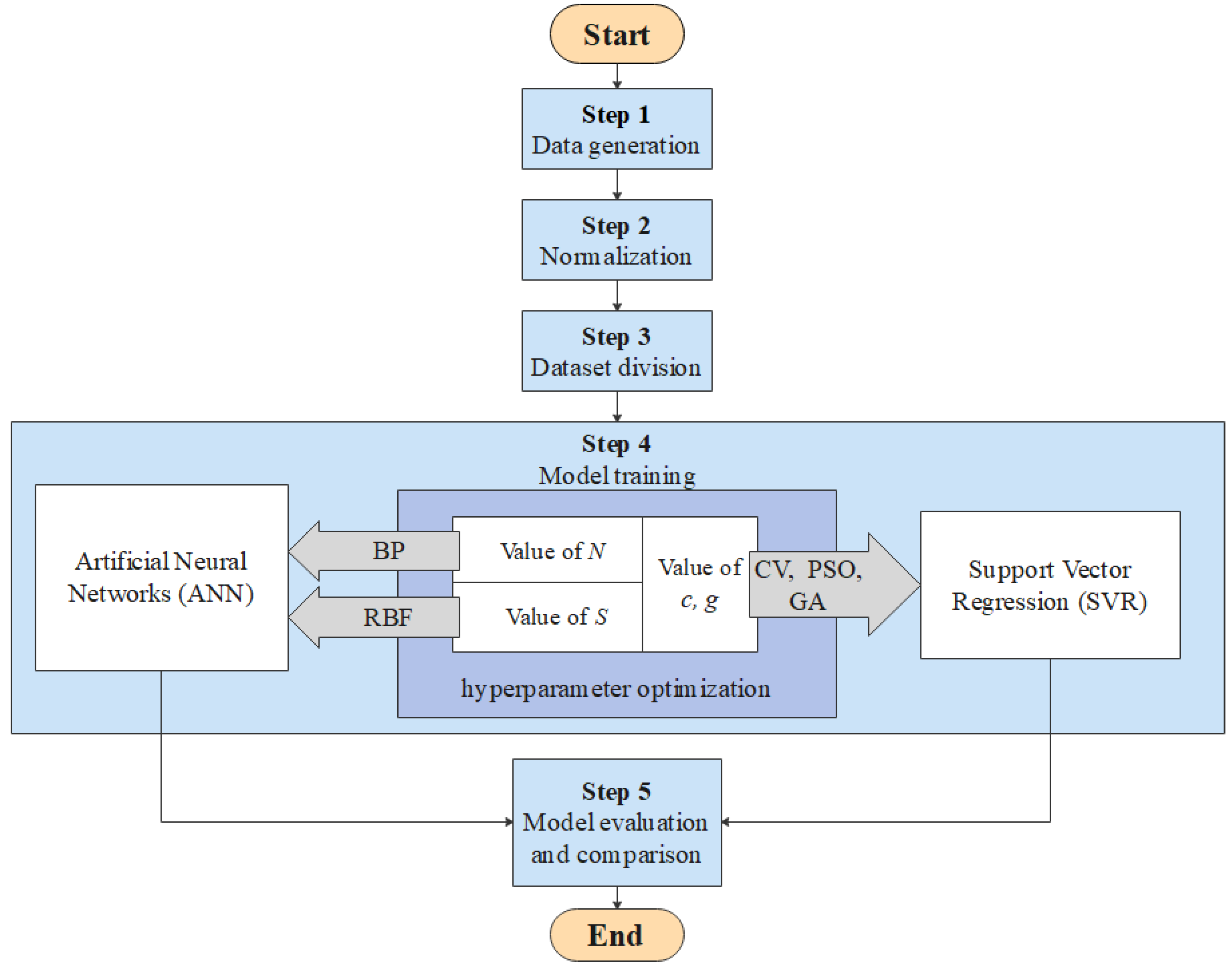
The general process of ML algorithms based on ANN and SVR for prediction is illustrated as follows, as shown in Figure 10.
Step 1 (Data generation): All qualitative variables are converted into quantitative variables. In this study, cooling in air (CIA) and cooling in water (CIW) in cooling method are indicated by 0 and 1, respectively.
Step 2 (Normalization): To eliminate the effect of scale, all the data must be normalized to improve the efficiency so that the range of processed data is within [0, 1]. The normalization formula is shown in Equation (4). [49]:
X i = x i m i n ( x i ) m a x ( x i ) m i n ( x i )
where Xi is the normalized data, min(xi) is the minimum of the un-normalized value, and max(xi) is the maximum of the un-normalized value.
Step 3 (Dataset division): To avoid overfitting, these data are randomly divided into two parts [50], with 5/6 and 1/6 of the data for training and testing the model, respectively. The training set is used for training and hyperparameter optimization, and the test set is used to evaluate the prediction accuracy of this model.
Step 4 (Model training): With the software of MATLAB R2021a, ANN and SVR algorithms are utilized in model training, and the hyperparameter optimization is carried out. Each objective hyperparameter is adjusted while keeping all others fixed.
Step 5 (Model evaluation and comparison): Other than R2, the mean square error (mse) [51] is also a widely used statistical metric to evaluate the prediction accuracy of ML, which measures the difference between the predicted values and the true values, as shown in Equation (5).
mse = i = 1 n ( y i y ^ i ) 2 n
where, y ^ i and yi are the ith true and predicted values, respectively, and n is the number of total data. By presenting R2 and mse values, the prediction accuracy of different methods can be compared.

3.2. Artificial Neural Network (ANN)

Both feedforward neural networks trained with the Levenberg–Marquardt backpropagation algorithm (ANN_BP) [52,53] and radial basis function neural network (ANN_RBF) [54] are popular neural networks with high predictive performance in recent studies. Their basic structures are similar, generally composed of the input layer, hidden layer and output layer [55]. Although the most difference is in the hidden layer, where ANN_RBF uses the RBF kernel as a transfer function in it [56], while ANN_BP uses the Sigmoid function [52].

3.2.1. ANN_BP

In the feedforward neural network, backpropagation solves problems related to complex networks and nonlinear functions. Figure 11 shows the basic principle of ANN_BP. The training process consists of two steps, namely, feed forward and backpropagation, where the ANN_BP model could be optimized by constantly adjusting the weight of neurons (w) and bias function (β) based on the error between calculated values and actual values [57] when the structure is basically fixed. The bias metrics in ANN_BP play a similar role as ε in OLS regression.
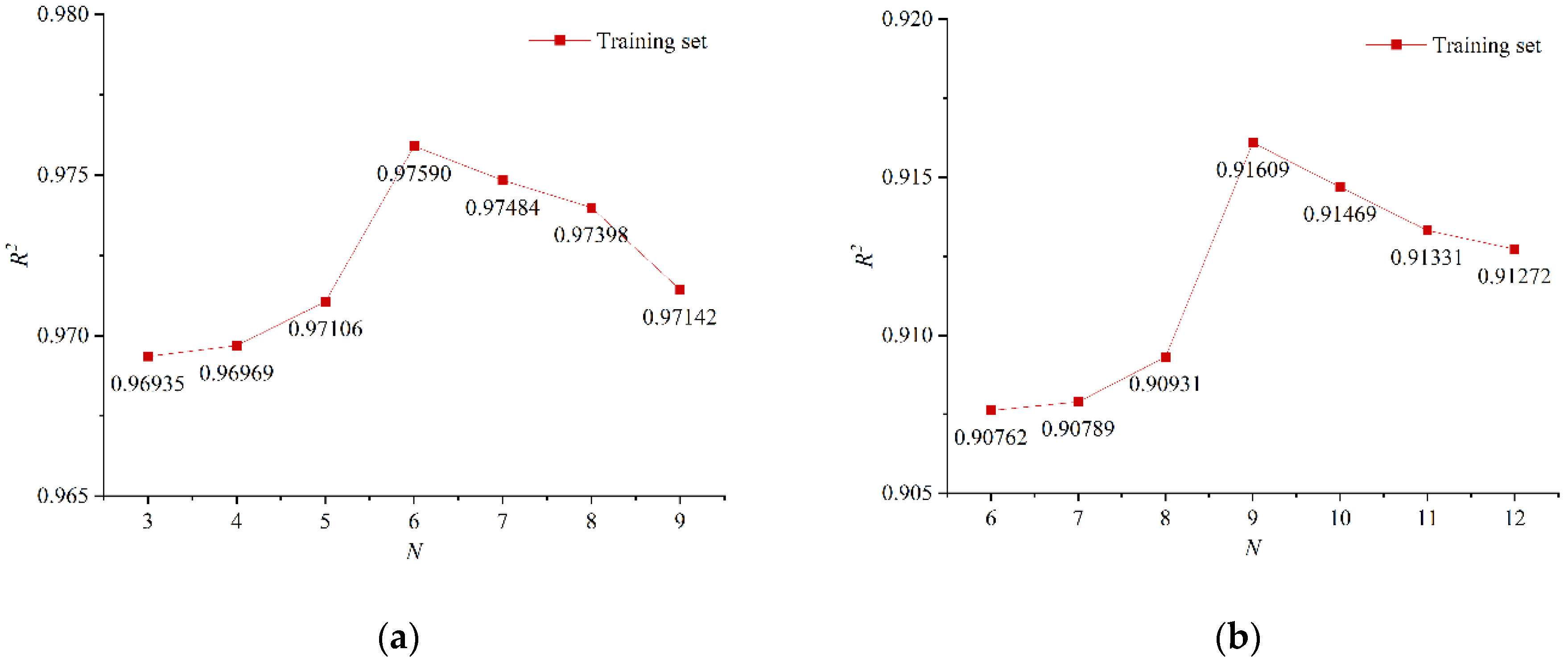
In most studies, the critical hyperparameters in the ANN_BP algorithm are the number of layers and the number of hidden neurons. Other hyperparameters are defined as follows: choose the Sigmoid function as the activation function, since all the data fall in [0, 1] after normalization, and the Sigmoid function ranges from 0 to 1 [58]. According to Li et al. [59], previous studies adopted either 1 or 2 hidden layers. Considering the computational efficiency, this paper chose one hidden layer first. The optimalization of the number of neurons (N) is a trial-and-error process. In order to eliminate the random error of dataset division and find the appropriate N, many trials are used to obtain the average statistical metric of each training set. In this study, ten trials are adopted. The influence of N (3~9) on prediction accuracy for TVu/20Vu ratio is presented in Figure 12a, which shows an upward and then downward trend. The results from sensitivity analysis indicate that the best performance network for TVu/20Vu ratio is with 6 neurons, where the average R2 value of the training set is 0.97590. After hyperparameter optimalization, the test set is used to assess the prediction accuracy [60], and the average R2 value of the test set is 0.97216. The influence of N (6~12) on prediction accuracy for the TVe20Ve ratio is presented in Figure 12b. It shows when N equals 9, the average R2 of the training set reaches the maximum value of 0.91609, where that of the test set is 0.91891.

3.2.2. ANN_RBF

ANN_RBF has the advantage of nonlinearity analysis when solving prediction problems, and the spread of each neuron (S) is a key hyperparameter [55], related to the Gaussian basis function in the hidden layers [57]. The larger the S is, the smoother the curve-fitting will be, but the approximation error will be larger. The smaller the S is, the less smooth the approximation process of ANN_RBF will be, and the poor performance even leads to over-fitting phenomenon [55]. Therefore, the hyperparameter optimalization of S value is required. Similarly, average R2 values are calculated using the results of ten randomized trials for choosing the best S value.
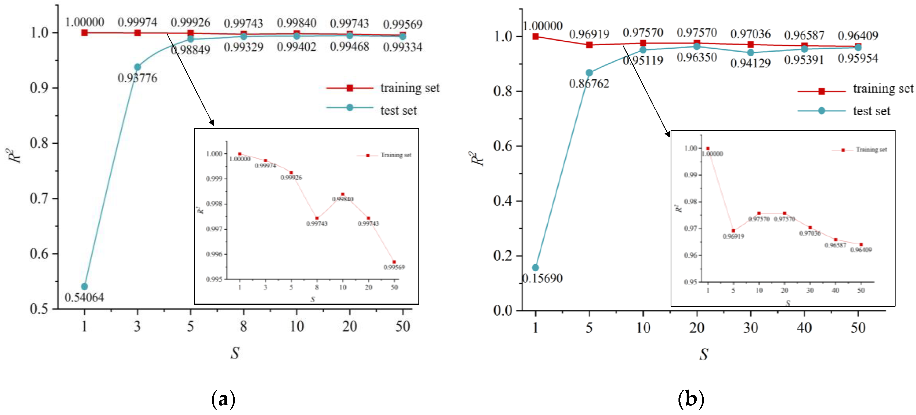
When building neural networks of the small-sample set, over-fitting phenomenon could be caused [61], which can be seen in Figure 13. When S is set as 1, the average R2 values of training set are both infinitely close to or equal to 1 for TVu/20Vu radio and TVe/20Ve ratio, while those of test set showing poor prediction performance, with 0.54064 and 0.15690, respectively. Therefore, following the approach adopted by Ref. [55], the parameter S is optimized by considering both training sets and test sets in case of overfitting. In Figure 13a, S = 1~50, the blue line rises faster with the fall of the red line, which indicates that a larger S has influence more on the prediction accuracy of test set (the blue line) than that of training set (the red line), for TVu/20Vu ratio. When S equals to 10, the average R2 value of training set is 0.99840, where the red line rises slightly and then keeps dropping, and R2 value of test set increases at a high level of 0.99402, showing the predicted and true data are quite well matched of both training and test set. The similar regular can be seen in Figure 13b for TVe/20Ve ratio, within the studied range of S (1~50), and the best choice of S is 20. The results of R2 values for the two parts of training and test are 0.97570 and 0.96350, respectively.

3.3. Support Vector Regression (SVR)

The regression and prediction accuracy of the SVR model is highly affected by the hyperparameter settings. Specifically, penalty hyperparameter c, and the key hyperparameter g of the RBF kernel function are the most significant [50]. The optimalization of c should avoid excessive learning and incomplete searching phenomenon [62]. Hyperparameter g is about the strength of the interaction between different support vectors, which affects the prediction efficiency and accuracy [63]. As predictive results of SVR are sensitive to the hyperparameter tuning, many common algorithms are used as hyperparameter optimization methods including cross-validation (CV) [64], particle swarm optimization (PSO) [65] and genetic algorithm (GA) [66]. Therefore, these three methods are all adopted in this study.

3.3.1. SVR+CV

To avoid overfitting, the k-fold cross-validation of the dataset is needed to evaluate the model performance during the process of training [64], and 5-fold is used in this study. The iterative process is repeated until the algorithm satisfies the termination condition, namely, the error convergence rate [67], which is the difference between two adjacent predicted values. In this study, it is set to be less than 10−4 [68]. The result of hyperparameter optimalization for TVu/20Vu ratio shows that the best c is 1.00000 and the best g is 0.17678. Similarly, the best c and g values for TVe/20Ve ratio are 0.70711 and 0.25000, respectively. Finally, the average R2 values of the test set for TVu/20Vu ratio and TVe/20Ve ratio, are 0.98613 and 0.91172, respectively.

3.3.2. SVR+PSO

The particle swarm optimization algorithm (PSO) is inspired by the behaviors of animals, which uses the updated particle swarm to find the best global and local positions [69]. Here, each particle represents a possible solution for the algorithm. PSO shows good performance in solving SVR optimization problems [65], and it is utilized in this part.
In this study, with a particle swarm size of 20 [70] and a maximum of 200 iterations [71], proper conditions can be preliminarily set through a 5-fold cross-validation method. The inertia factor w(p) is 0.1, whose function is to prevent quick convergence [71]. The learning factors (c1 = 1.5 [69] and c2 = 1.7) are considered as two accelerations adjusting the relative velocities when finding the best positions [63]. This paper uses the LIBSVM (Library for support vector machines) format for hyperparameter optimization in the SVR+PSO algorithm [72], where the error convergence rate is less than 10−4 [68]. Results show that for TVu/20Vu ratio, the best c is 100 and the best g is 0.50312 while the best c is 19.53590 and the best g is 0.92395 for TVe/20Ve ratio. Using these optimal hyperparameters, the results of average R2 values of each test set can be obtained, with 0.99445 and 0.94714 for TVu/20Vu ratio and TVe/20Ve ratio, respectively.

3.3.3. SVR+GA

GA is used to automatically determine the optimal or approximate optimal hyperparameters in the SVR model [66]. The advantage of GA is its powerful global optimization function, which guarantees the prediction accuracy and application range of the SVR model.
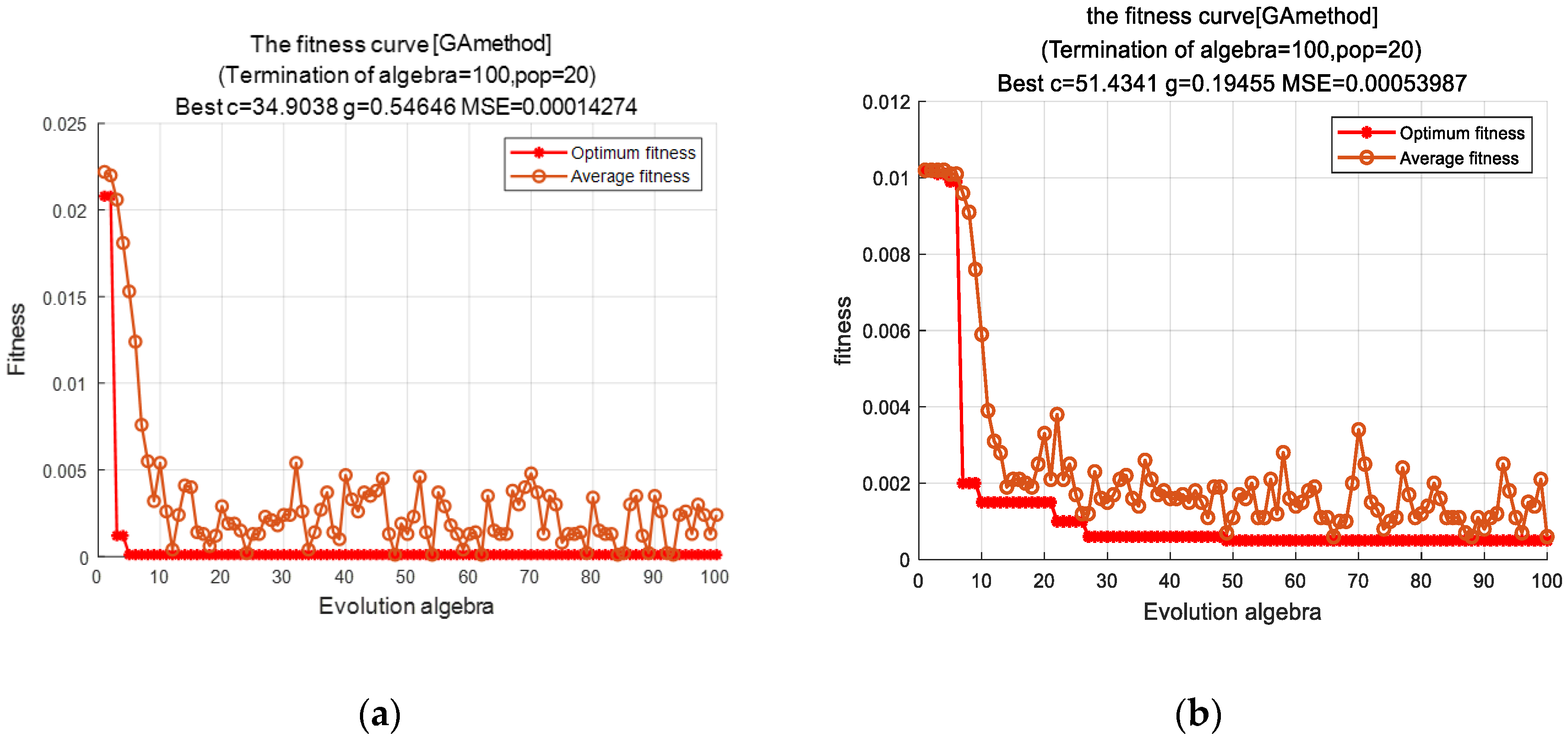
The optimization process with GA is defined with a population of 20 individuals in 100 iterations, for 5-fold cross-validation. ggap is the proportion of superior individuals selected from the parent generation. In this paper, the length of the individual ggap is 0.9, which means the proportion of individuals replaced by the next generation is 10%. The LIBSVM format is a significant step, which is utilized to find appropriate hyperparameters directly [72]. The SVR+GA algorithm is terminated when the rate of error convergence is less than 10−4 [68]. The curves of fitness function for TVu/20Vu ratio are shown in Figure 14a, where the optimization procedure converges after 4 iterations, showing best c is 34.90380 and best g is 0.54646. The same method can be used to find the suitable hyperparameters for TVe/20Ve ratio in Figure 14b, which shows the best c of 51.43410 and the best g of 0.19455 after 27 iterations. Using the optimal hyperparameters of c and g with the stable condition, the average R2 values of test set for TVu/20Vu ratio and TVe/20Ve ratio are 0.99406 and 0.99472, respectively. It is observed that, both the R2 values of SVR+GA are close to 1, which preliminarily indicates that the SVR model could provide accurate predictions for the objective functions after the process of hyperparameter tuning with GA.

4. Predicted Results

4.1. Prediction of Ultimate Resistance (TVu/20Vu Ratio)

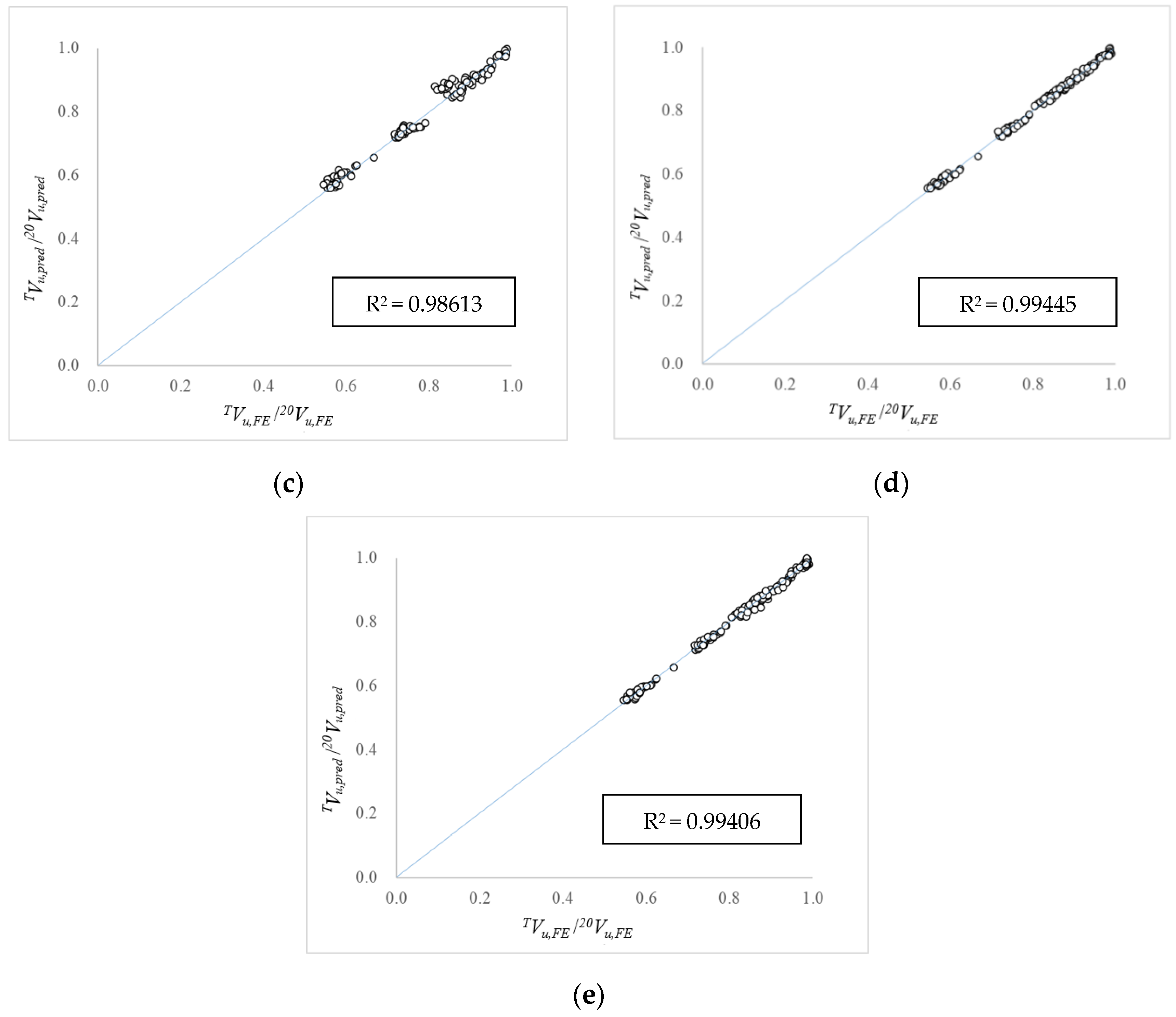
After optimalization of hyperparameters, the structures of ML are confirmed, and the prediction accuracy is calculated using a test set [60]. Figure 15 presents the TVu,pred/20Vu,predTVu,FE/20Vu,FE scatter plots for ANN_BP, ANN_RBF, SVR+CV, SVR+PSO and SVR+GA, respectively. In addition, Table 3 lists the average R2 and mse values as the regular statistical error indicators. It is visible that a majority of the points fall on the diagonal line of these five plots, indicating that the true values (Vu,FE) and predicted values (Vu,pred) fit well. The best agreement is seen in ANN_RBF, SVR+PSO and SVR+GA, where the averaged R2 values are 0.99402, 0.99445 and 0.99406, respectively. Additionally, their mse values are 0.00018, 0.00021 and 0.00015, respectively, lower than that of the two models. It could be concluded that SVR and ANN models after hyperparameter optimization can reach higher levels of predictive accuracy than the OLS model, especially for ANN_RBF, SVR+PSO and SVR+GA.

4.2. Prediction of Effective Service Resistance (TVe/20Ve)

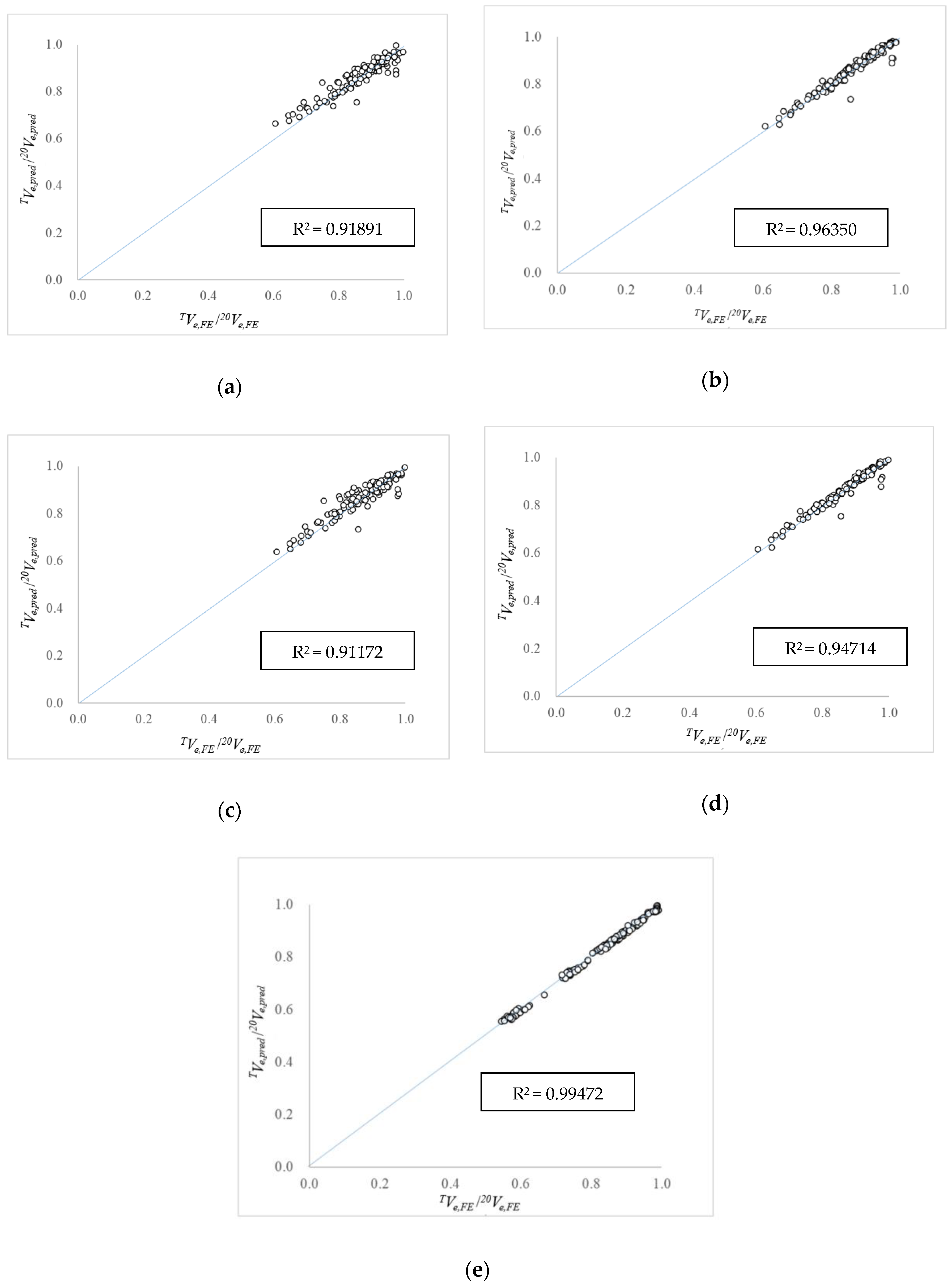
Figure 16 the TVe,pred/20Ve,predTVe,FE/20Ve,FE scatter plots for ANN_BP, ANN_RBF, SVR+CV, SVR+PSO and SVR+GA, respectively. It also presents R2 values of each test set in these five algorithms, which can be seen that only a few predicted values differ slightly from the true values, and the other predicted values are very close to true values. The specific R2 and mse values of each test set with different algorithms are calculated and compared for determining the accuracy, and the results are shown in Table 4. It could be concluded that the algorithm combined with SVR and GA has a better prediction effect for TVe/20Ve ratio, where R2 value is 0.99472 and mse value is 0.00013.

5. Discussions and Future Works

Comparing the predicted results in Table 2,Table 3,Table 4, it could be concluded that ML algorithms represented by ANN and SVR can obtain better forecasting performance than the traditional method of OLS regression. Apparently, OLS regression lacks the learning process to eliminate interference values and errors, while both ANN and SVR have the ability of nonlinear processing, which ensures that sufficient information of input variables and output variables could be fully utilized.
Basically, all the predictive results by ML are within a reasonable range, since the R2 values vary between 0.91891 and 0.99472 while mse values vary between 0.00013 and 0.00261. The predictive accuracy could be compared with that of other similar research. For example, the R2 value of SVR is 0.9470, when evaluating the compressive strength of the concrete samples [50]. Concurrently, the R2 value of ANN is 0.82 when predicting the strength of different soils [73]. As for the accuracy of ANN, mse values for moment and rotation prediction of tested connections are 0.63 and 0.0021, respectively [74]. Therefore, it could be concluded that the predictive accuracy of the ML models in this paper is satisfying.
In terms of the comparisons between the two methods of ANN, ANN_RBF achieves higher precision than ANN_BP, for it uses the RBF kernel as a transfer function [57], which is the best of all kernel functions [75]. Within all the models of SVR, SVR+PSO seems to be the most efficient and accurate for the hyperparameter optimization of the TVu/20Vu ratio prediction, while SVR+GA exhibits the best of the TVe/20Ve ratio prediction. Basically, SVR+GA performs the highest accuracy in predicting both TVu/20Vu and TVe/20Ve ratio. Although both ANN_RBF and SVR+GA use the RBF kernel function and optimize the core hyperparameters, the prediction accuracy of SVR+GA is higher than that of ANN_RBF for TVu/20Vu ratio and TVe/20Ve ratio, since SVR has the characteristics of strong generalization ability with small samples [76], which is the case in this study. Therefore, when carrying out a similar prediction, the SVR+GA algorithm is expected to provide a more practical guarantee in terms of prediction accuracy.
As for the correlation analysis, the results of ICE can be linked with the conclusions in OLS regression, where the influence of each independent variable on the dependent variable shows the same direction. In OLS regression, the influence of four parameters on the dependent variable is considered simultaneously and one scatter plot is drawn. However, with ICE, the influence of one parameter on the dependent variable is considered separately and the corresponding scatter plot is drawn as four plots. In practice, both methods could be used to predict the general relationships between dependent variables and independent variables, but the detailed trends shown in ICE seem to be clearer than those in OLS regression, and ICE has a better ability to show the potential complexity of the correlations.
For future studies, the numerical studies could be further improved by considering the creep effects. Additionally, to enhance the generalization ability of machine learning approaches, increasing the quantity of data could be an efficient measure. In addition, the process of hyperparameter tuning could be optimized so that the evaluation process significantly improves in accuracy. Furthermore, machine learning methods should be used in solving other problems similar to the case of this study, especially for the capacity prediction under complex circumstances. Finally, it should be noticed that the results of Q690 plate girder after fire in this study are based on the following limitation: hw/tw between 100 and 300, a/hw ratio within 0.5~2, exposure temperature 700~900 °C and cooling method should be CIA or CIW.

6. Conclusions

Mechanical properties of Q690 HSS performed significant effects on the resistance of plate girders’ developing post-buckling capacity. When the plate girder did not collapse after a fire its residual resistant capacity should be evaluated. The exposure temperature and cooling method performed noteworthy effects on the mechanical properties of Q690 HSS, which also influenced the resistance of the plate girder. Considering that there were many influencing variables, it is very difficult to determine the residual resistance of the Q690 HSS plate girder effectively after the fire through the traditional predictive method. Therefore, the machine learning method was innovatively used in this study. Post-fire resistance of Q690 HSS plate girders was investigated through material tests, FE analysis and parametric study. Additionally, the prediction of the reduction factor of post-fire resistance with machine learning methods shows better performance than that with traditional OLS regression, which could be conveniently used in the evaluation of the residual resistance of the Q690 HSS plate girder after fire. The main conclusions of this research include the following:
  • The exposure temperature is the most significant parameter for the reduction factor by imposing a negative effect on the ultimate resistance and effective service resistance of Q690 HSS plate girders while cooling in water (CIW) is a more beneficial cooling method than cooling in the air (CIA) in terms of the residual resistance. Basically, the small impact of hw/tw ratio and a/hw ratio on the resistance reduction is seen.
  • The R2 values of the OLS regression method for TVu/20Vu ratio and TVe/20Ve ratio are 0.7860 and 0.6954, respectively. The accuracy of fitting and calculating the statistical metric is not high enough for predictions.
  • The results show that effective algorithms (i.e., PSO and GA) can be used to automatically optimize the core hyperparameters, which may have higher efficiency than the trial-and-error process relying on human experience.
  • Specifically, SVR+PSO seems to be the most accurate algorithm when predicting TVu/20Vu ratio, where R2 value of the test set is 0.99445 and mse value is 0.00021. SVR+GA exhibits the best prediction of TVe/20Ve ratio with an R2 value of 0.99472 and mse value of 0.00013. Considering the accuracy in prediction, the SVR+GA algorithm provides the best performance for both TVu/20Vu ratio and TVe/20Ve ratio.

Supplementary Materials

The following supporting information can be downloaded at: https://www.mdpi.com/article/10.3390/buildings12091481/s1, Table S1: Reduction factors for the stress properties of steel, Table S2: Geometrical dimensions of numerical model, Table S3: Numerical analysis results: 20 °C, Table S4: Numerical analysis results: 700 °C and with CIA/ CIW, Table S5: Numerical analysis results: 800 °C and with CIA/CIW.

Author Contributions

Conceptualization, G.L. and N.W.; data curation, J.L. and X.X.; funding acquisition, G.L. and N.W.; investigation, J.L. and X.X.; methodology, N.W. and X.X.; project administration, G.L. and N.W.; software, Y.T.; supervision, X.X.; validation, Y.T.; visualization, Y.T.; writing—original draft, J.L.; writing—review & editing, N.W. All authors have read and agreed to the published version of the manuscript.

Funding

This study is financially supported by the National Natural Science Foundation of China (grant No. 52108115).

Data Availability Statement

Not applicable.

Conflicts of Interest

The authors declare no conflict of interest.

References

  1. Yoo, C.H.; Lee, S.C. Mechanics of Web Panel Postbuckling Behavior in Shear. J. Struct. Eng. 2006, 132, 1580–1589. [Google Scholar] [CrossRef]
  2. Kim, Y.D.; White, D.W. Transverse Stiffener Requirements to Develop Shear-Buckling and Postbuckling Resistance of Steel I-Girders. J. Struct. Eng. 2014, 140, 04013098. [Google Scholar] [CrossRef]
  3. Hassanein, M. Finite element investigation of shear failure of lean duplex stainless steel plate girders. Thin-Walled Struct. 2011, 49, 964–973. [Google Scholar] [CrossRef]
  4. Alinia, M.; Gheitasi, A.; Shakiba, M. Postbuckling and ultimate state of stresses in steel plate girders. Thin-Walled Struct. 2011, 49, 455–464. [Google Scholar] [CrossRef]
  5. Choi, Y.S.; Kim, D.; Lee, S.C. Ultimate shear behavior of web panels of HSB800 plate girders. Constr. Build. Mater. 2015, 101, 828–837. [Google Scholar] [CrossRef]
  6. Xue, X.Y.; Zhou, X.; Shi, Y.; Xiang, Y. Ultimate shear resistance of S600E high-strength stainless steel plate girders. J. Constr. Steel Res. 2021, 179, 106535. [Google Scholar] [CrossRef]
  7. Xiao, Y.; Xue, X.Y.; Sun, F.F.; Li, G.Q. Intermediate transverse stiffener requirements of high-strength steel plate girders considering postbuckling capacity. Eng. Struct. 2019, 196, 109289. [Google Scholar] [CrossRef]
  8. Xiao, Y.; Xue, X.Y.; Sun, F.F.; Li, G.Q. Postbuckling shear capacity of high-strength steel plate girders. J. Constr. Steel Res. 2018, 150, 475–490. [Google Scholar] [CrossRef]
  9. Azizinamini, A.; Hash, J.B.; Yakel, A.J.; Farimani, R. Shear Capacity of Hybrid Plate Girders. J. Bridg. Eng. 2007, 12, 535–543. [Google Scholar] [CrossRef]
  10. Hua, J.; Xue, X.; Huang, Q.; Shi, Y.; Deng, W. Post-fire performance of high-strength steel plate girders developing post-buckling capacity. J. Build. Eng. 2022, 52, 104442. [Google Scholar] [CrossRef]
  11. Shi, Y.; Luo, Z.; Zhou, X.; Xue, X.; Xiang, Y. Post-fire performance of bonding interface in explosion-welded stainless-clad bimetallic steel. J. Constr. Steel Res. 2022, 193, 107285. [Google Scholar] [CrossRef]
  12. Hua, J.; Wang, F.; Xue, X. Study on fatigue properties of post-fire bimetallic steel bar with different cooling methods. Structures 2022, 40, 633–645. [Google Scholar] [CrossRef]
  13. Hua, J.; Yang, Z.; Wang, F.; Xue, X.; Wang, N.; Huang, L. Relation between the Metallographic Structure and Mechanical Properties of a Bimetallic Steel Bar after Fire. J. Mater. Civ. Eng. 2022, 34, 04022193. [Google Scholar] [CrossRef]
  14. Naser, M.; Kodur, V. A probabilistic assessment for classification of bridges against fire hazard. Fire Saf. J. 2015, 76, 65–73. [Google Scholar] [CrossRef]
  15. Hua, J.; Wang, F.; Yang, Z.; Xue, X.; Huang, L.; Chen, Z. Low-cycle fatigue properties of bimetallic steel bars after exposure to elevated temperature. J. Constr. Steel Res. 2021, 187, 106959. [Google Scholar] [CrossRef]
  16. Shi, Y.; Luo, Z.; Zhou, X.; Xue, X.; Li, J. Post-fire mechanical properties of titanium–clad bimetallic steel in different cooling approaches. J. Constr. Steel Res. 2022, 191, 107169. [Google Scholar] [CrossRef]
  17. Kodur, V.; Naser, M. Importance factor for design of bridges against fire hazard. Eng. Struct. 2013, 54, 207–220. [Google Scholar] [CrossRef]
  18. Naser, M. Deriving temperature-dependent material models for structural steel through artificial intelligence. Constr. Build. Mater. 2018, 191, 56–68. [Google Scholar] [CrossRef]
  19. Wang, W.; Zhou, H.; Xu, L. Creep buckling of high strength Q460 steel columns at elevated temperatures. J. Constr. Steel Res. 2019, 157, 414–425. [Google Scholar] [CrossRef]
  20. Zhou, X.; Xue, X.; Shi, Y.; Xu, J. Post-fire mechanical properties of Q620 high-strength steel with different cooling methods. J. Constr. Steel Res. 2021, 180, 106608. [Google Scholar] [CrossRef]
  21. Wang, W.; Liu, T.; Liu, J. Experimental study on post-fire mechanical properties of high strength Q460 steel. J. Constr. Steel Res. 2015, 114, 100–109. [Google Scholar] [CrossRef]
  22. Li, G.; Lü, H.; Zhang, C. Experimental research on post-fire mechanical properties of Q690 steel. Jianzhu Jiegou Xuebao/J. Build. Struct. 2017, 38, 109–116. [Google Scholar] [CrossRef]
  23. Qiang, X.; Bijlaard, F.S.; Kolstein, H. Post-fire mechanical properties of high strength structural steels S460 and S690. Eng. Struct. 2012, 35, 1–10. [Google Scholar] [CrossRef]
  24. Thai, H.-T. Machine learning for structural engineering: A state-of-the-art review. Structures 2022, 38, 448–491. [Google Scholar] [CrossRef]
  25. Sun, H.; Burton, H.V.; Huang, H. Machine learning applications for building structural design and performance assessment: State-of-the-art review. J. Build. Eng. 2020, 33, 101816. [Google Scholar] [CrossRef]
  26. Salehi, H.; Burgueño, R. Emerging artificial intelligence methods in structural engineering. Eng. Struct. 2018, 171, 170–189. [Google Scholar] [CrossRef]
  27. Zarringol, M.; Thai, H.-T.; Naser, M. Application of machine learning models for designing CFCFST columns. J. Constr. Steel Res. 2021, 185, 106856. [Google Scholar] [CrossRef]
  28. Hozjan, T.; Turk, G.; Srpčič, S. Fire analysis of steel frames with the use of artificial neural networks. J. Constr. Steel Res. 2007, 63, 1396–1403. [Google Scholar] [CrossRef]
  29. Almasabha, G.; Alshboul, O.; Shehadeh, A.; Almuflih, A.S. Machine Learning Algorithm for Shear Strength Prediction of Short Links for Steel Buildings. Buildings 2022, 12, 775. [Google Scholar] [CrossRef]
  30. Dulce-Chamorro, E.; Martinez-De-Pison, F.J. An advanced methodology to enhance energy efficiency in a hospital cooling-water system. J. Build. Eng. 2021, 43, 102839. [Google Scholar] [CrossRef]
  31. Deng, Z.; Chen, Q. Artificial neural network models using thermal sensations and occupants’ behavior for predicting thermal comfort. Energy Build. 2018, 174, 587–602. [Google Scholar] [CrossRef]
  32. Deng, F.; He, Y.; Zhou, S.; Yu, Y.; Cheng, H.; Wu, X. Compressive strength prediction of recycled concrete based on deep learning. Constr. Build. Mater. 2018, 175, 562–569. [Google Scholar] [CrossRef]
  33. GB/T 228-2010; Metallic Materials—Tensile Testing—Part 1: Method of Test at Room Temperature. China Standard Press: Beijing, China, 2010.
  34. Song, L.-X.; Li, G.-Q. Processing and cooling effects on post-fire mechanical properties of high strength structural steels. Fire Saf. J. 2021, 122, 103346. [Google Scholar] [CrossRef]
  35. Hua, J.; Wang, F.; Xue, X.; Ding, Z.; Sun, Y.; Xiao, L. Ultra-low cycle fatigue performance of Q690 high-strength steel after exposure to elevated temperatures. J. Build. Eng. 2022, 57, 104832. [Google Scholar] [CrossRef]
  36. Hua, J.; Yang, Z.; Zhou, F.; Hai, L.; Wang, N.; Wang, F. Effects of exposure temperature on low–cycle fatigue properties of Q690 high–strength steel. J. Constr. Steel Res. 2022, 190, 107159. [Google Scholar] [CrossRef]
  37. Saliba, N.; Real, E.; Gardner, L. Shear design recommendations for stainless steel plate girders. Eng. Struct. 2014, 59, 220–228. [Google Scholar] [CrossRef]
  38. CEN. Eurocode 3: Design of Steel Structures, Part 1–5: Plated Structural Elements; European Committee for Standardisation: Brussels, Belgium, 2006. [Google Scholar]
  39. AASHTO; AWS. Bridge Welding Code, ANSI/AASHTO/AWS D1.5M/D1.5:2002; American Association of State Highway and Transportation Officials, Inc.: Washington, DC, USA; American Welding Society: Miami, FL, USA, 2002. [Google Scholar]
  40. Hassanein, M. Imperfection analysis of austenitic stainless steel plate girders failing by shear. Eng. Struct. 2010, 32, 704–713. [Google Scholar] [CrossRef]
  41. Ghadami, A.; Broujerdian, V. Shear behavior of steel plate girders considering variations in geometrical properties. J. Constr. Steel Res. 2018, 153, 567–577. [Google Scholar] [CrossRef]
  42. Sinur, F.; Beg, D. Moment–shear interaction of stiffened plate girders—Tests and numerical model verification. J. Constr. Steel Res. 2013, 85, 116–129. [Google Scholar] [CrossRef]
  43. EN 1993-1-5; Eurocode 3: Design of Steel Strcture-Part 1.5: Plated Structural Elements. European Committee for Standarlization: Brussels, Belgium, 2010.
  44. GB 50017-2007; Standard for Design of Steel Structures. China Architecture & Building Press: Beijing, China, 2017.
  45. Goldstein, A.; Kapelner, A.; Bleich, J.; Pitkin, E. Peeking Inside the Black Box: Visualizing Statistical Learning with Plots of Individual Conditional Expectation. J. Comput. Graph. Stat. 2015, 24, 44–65. [Google Scholar] [CrossRef] [Green Version]
  46. Ji, S.; Lee, B.; Yi, M.Y. Building life-span prediction for life cycle assessment and life cycle cost using machine learning: A big data approach. Build. Environ. 2021, 205, 108267. [Google Scholar] [CrossRef]
  47. Rustam, F.; Reshi, A.A.; Mehmood, A.; Ullah, S.; On, B.-W.; Aslam, W.; Choi, G.S. COVID-19 Future Forecasting Using Supervised Machine Learning Models. IEEE Access 2020, 8, 101489–101499. [Google Scholar] [CrossRef]
  48. Aziminezhad, M.; Mahdikhani, M.; Memarpour, M.M. RSM-based modeling and optimization of self-consolidating mortar to predict acceptable ranges of rheological properties. Constr. Build. Mater. 2018, 189, 1200–1213. [Google Scholar] [CrossRef]
  49. Zhang, F.; Bales, C.; Fleyeh, H. From time series to image analysis: A transfer learning approach for night setback identification of district heating substations. J. Build. Eng. 2021, 43, 102537. [Google Scholar] [CrossRef]
  50. Huang, J.; Sun, Y.; Zhang, J. Reduction of computational error by optimizing SVR kernel coefficients to simulate concrete compressive strength through the use of a human learning optimization algorithm. Eng. Comput. 2022, 38, 3151–3168. [Google Scholar] [CrossRef]
  51. Sanhudo, L.; Rodrigues, J.; Filho, V. Multivariate time series clustering and forecasting for building energy analysis: Application to weather data quality control. J. Build. Eng. 2020, 35, 101996. [Google Scholar] [CrossRef]
  52. Al-Shamiri, A.K.; Kim, J.H.; Yuan, T.-F.; Yoon, Y.S. Modeling the compressive strength of high-strength concrete: An extreme learning approach. Constr. Build. Mater. 2019, 208, 204–219. [Google Scholar] [CrossRef]
  53. Amoosoltani, E.; Ameli, A.; Jabari, F.; Asadi, S. Employing a hybrid GA-ANN method for simulating fracture toughness of RCC mixture containing waste materials. Constr. Build. Mater. 2020, 272, 121928. [Google Scholar] [CrossRef]
  54. Yilmaz, I.; Kaynar, O. Multiple regression, ANN (RBF, MLP) and ANFIS models for prediction of swell potential of clayey soils. Expert Syst. Appl. 2011, 38, 5958–5966. [Google Scholar] [CrossRef]
  55. Kang, F.; Li, J.; Zhao, S.; Wang, Y. Structural health monitoring of concrete dams using long-term air temperature for thermal effect simulation. Eng. Struct. 2018, 180, 642–653. [Google Scholar] [CrossRef]
  56. Gujar, R.; Vakharia, V. Prediction and validation of alternative fillers used in micro surfacing mix-design using machine learning techniques. Constr. Build. Mater. 2019, 207, 519–527. [Google Scholar] [CrossRef]
  57. Bakeer, A.; Magdy, G.; Chub, A.; Bevrani, H. A sophisticated modeling approach for photovoltaic systems in load frequency control. Int. J. Electr. Power Energy Syst. 2022, 134, 107330. [Google Scholar] [CrossRef]
  58. Degtyarev, V.V. Neural networks for predicting shear strength of CFS channels with slotted webs. J. Constr. Steel Res. 2020, 177, 106443. [Google Scholar] [CrossRef]
  59. Li, S.; Liew, J.R.; Xiong, M.-X. Prediction of fire resistance of concrete encased steel composite columns using artificial neural network. Eng. Struct. 2021, 245, 112877. [Google Scholar] [CrossRef]
  60. Ferreira, F.P.V.; Shamass, R.; Limbachiya, V.; Tsavdaridis, K.D.; Martins, C.H. Lateral–torsional buckling resistance prediction model for steel cellular beams generated by Artificial Neural Networks (ANN). Thin-Walled Struct. 2021, 170, 108592. [Google Scholar] [CrossRef]
  61. Yigit, S. A machine-learning-based method for thermal design optimization of residential buildings in highly urbanized areas of Turkey. J. Build. Eng. 2021, 38, 102225. [Google Scholar] [CrossRef]
  62. Han, B.; Bian, X. A hybrid PSO-SVM-based model for determination of oil recovery factor in the low-permeability reservoir. Petroleum 2018, 4, 43–49. [Google Scholar] [CrossRef]
  63. Ni, L.; Jiang, J.; Pan, Y. Leak location of pipelines based on transient model and PSO-SVM. J. Loss Prev. Process Ind. 2013, 26, 1085–1093. [Google Scholar] [CrossRef]
  64. Vakharia, V.; Gujar, R. Prediction of compressive strength and portland cement composition using cross-validation and feature ranking techniques. Constr. Build. Mater. 2019, 225, 292–301. [Google Scholar] [CrossRef]
  65. Zhou, X.; Zi, X.; Liang, L.; Fan, Z.; Yan, J.; Pan, D. Forecasting performance comparison of two hybrid machine learning models for cooling load of a large-scale commercial building. J. Build. Eng. 2018, 21, 64–73. [Google Scholar] [CrossRef]
  66. Pirmohammad, S.; Marzdashti, S.E. Crashworthiness optimization of combined straight-tapered tubes using genetic algorithm and neural networks. Thin-Walled Struct. 2018, 127, 318–332. [Google Scholar] [CrossRef]
  67. Ben Chaabene, W.; Flah, M.; Nehdi, M.L. Machine learning prediction of mechanical properties of concrete: Critical review. Constr. Build. Mater. 2020, 260, 119889. [Google Scholar] [CrossRef]
  68. Jiang, W.; Xie, Y.; Li, W.; Wu, J.; Long, G. Prediction of the splitting tensile strength of the bonding interface by combining the support vector machine with the particle swarm optimization algorithm. Eng. Struct. 2020, 230, 111696. [Google Scholar] [CrossRef]
  69. Kookalani, S.; Cheng, B.; Xiang, S. Shape optimization of GFRP elastic gridshells by the weighted Lagrange ε-twin support vector machine and multi-objective particle swarm optimization algorithm considering structural weight. Structures 2021, 33, 2066–2084. [Google Scholar] [CrossRef]
  70. Truong, V.-H.; Kim, S.-E. A robust method for optimization of semi-rigid steel frames subject to seismic loading. J. Constr. Steel Res. 2018, 145, 184–195. [Google Scholar] [CrossRef]
  71. Khatibinia, M.; Jalaipour, M.; Gharehbaghi, S. Shape optimization of U-shaped steel dampers subjected to cyclic loading using an efficient hybrid approach. Eng. Struct. 2019, 197, 108874. [Google Scholar] [CrossRef]
  72. Chang, C.; Lin, C. LIBSVM: A Library for Support Vector Machines. ACM Trans. Intell. Syst. Technol. 2013, 2, 27. [Google Scholar] [CrossRef]
  73. Eyo, E.; Abbey, S. Machine learning regression and classification algorithms utilised for strength prediction of OPC/by-product materials improved soils. Constr. Build. Mater. 2021, 284, 122817. [Google Scholar] [CrossRef]
  74. Shah, S.; Sulong, N.R.; El-Shafie, A. New approach for developing soft computational prediction models for moment and rotation of boltless steel connections. Thin-Walled Struct. 2018, 133, 206–215. [Google Scholar] [CrossRef]
  75. Jueyendah, S.; Lezgy-Nazargah, M.; Eskandari-Naddaf, H.; Emamian, S. Predicting the mechanical properties of cement mortar using the support vector machine approach. Constr. Build. Mater. 2021, 291, 123396. [Google Scholar] [CrossRef]
  76. Yang, C.; Liu, J.; Zeng, Y.; Xie, G. Prediction of components degradation using support vector regression with optimized parameters. Energy Procedia 2017, 127, 284–290. [Google Scholar] [CrossRef]
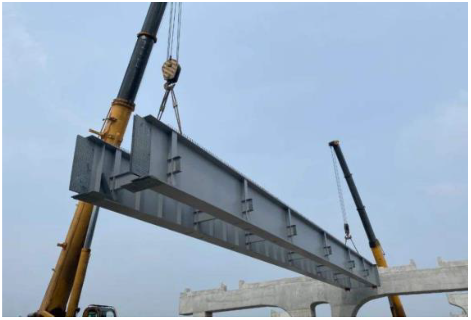
Figure 1. Steel plate girder in long-span structures.
Buildings 12 01481 g001
Figure 2. Dimensions of tensile coupon test specimen.
Buildings 12 01481 g002
Figure 3. Process of the material test (CIA: cooling in air; CIW: cooling in water).
Buildings 12 01481 g003
Figure 4. Results of the material test. (a) strain-stress curve; (b) microstructures.
Buildings 12 01481 g004
Figure 5. Numerical analysis. (a) FE model; (b) convergence study.
Buildings 12 01481 g005
Figure 6. Shear load-midspan displacement curves of P-1-250 with different exposure temperatures and cooling methods.
Buildings 12 01481 g006
Figure 7. Individual conditional expectation plots. (a) Results for TVu/20Vu ratio; (b) Results for TVe/20Ve ratio.
Buildings 12 01481 g007
Figure 8. Failure modes of numerical models: (a) 20 °C and without cooling treatment; (b) 900 °C and CIA; (c) 900 °C and CIW.
Buildings 12 01481 g008
Figure 9. Prediction of resistance reduction through linear regression. (a) TVu,pred/20Vu,predTVu,FE/20Vu,FE scatter plot; (b) TVe,pred/20Ve,predTVe,FE/20Ve,FE scatter plot.
Buildings 12 01481 g009
Figure 10. Flow chart of the machine learning methodology.
Buildings 12 01481 g010
Figure 11. Technological structure of ANN_BP.
Buildings 12 01481 g011
Figure 12. Influences of the number of neurons (N) on R2 on the training set. (a) TVu/20Vu ratio; (b) TVe/20Ve ratio.
Buildings 12 01481 g012
Figure 13. Influences of spread (S) on R2 of training set and test set. (a) TVu/20Vu ratio; (b) TVe/20Ve ratio.
Buildings 12 01481 g013
Figure 14. The fitness curve of GA method. (a) Results for TVu/20Vu ratio; (b) Results for TVe/20Ve ratio.
Buildings 12 01481 g014
Figure 15. Training and test results of machine learning methodology for TVu/20Vu ratio. (a) TVu,pred/20Vu,predTVu,FE/20Vu,FE scatter plot of ANN_BP; (b) TVu,pred/20Vu,predTVu,FE/20Vu,FE scatter plot of ANN_RBF; (c) TVu,pred/20Vu,predTVu,FE/20Vu,FE scatter plot of SVR+CV; (d) TVu,pred/20Vu,predTVu,FE/20Vu,FE scatter plot of SVR+PSO; (e) TVu,pred/20Vu,predTVu,FE/20Vu,FE scatter plot of SVR+GA.
Buildings 12 01481 g015aBuildings 12 01481 g015b
Figure 16. Training and test results of machine learning methodology for TVe/20Ve. (a) TVe,pred/20Ve,predTVe,FE/20Ve,FE scatter plot of ANN_BP; (b) TVe,pred/20Ve,predTVe,FE/20Ve,FE scatter plot of ANN_RBF; (c) TVe,pred/20Ve,predTVe,FE/20Ve,FE scatter plot of SVR+CV; (d) TVe,pred/20Ve,predTVe,FE/20Ve,FE scatter plot of SVR+PSO; (e) TVe,pred/20Ve,predTVe,FE/20Ve,FE scatter plot of SVR+GA.
Buildings 12 01481 g016
Table 1. Q690 HSS chemical composition.
ElementSiMnCBCrMoTiNiPSNb
wt.%0.151.570.070.0010.010.020.090.010.0100.0020.001
Table 2. ANOVA response for the linear regression model.
Independent VariablesDependent Variables
TVu/20Vu RatioTVe/20Ve Ratio
Coefp-ValueCoefp-Value
X1: hw/tw−0.02460.098 *0.0639<0.001 ***
X2: a/hw−0.01830.085 *0.048<0.001 ***
X3: exposure temperature T−0.2583<0.001 ***−0.1857<0.001 ***
X4: cooling method0.1582<0.001 ***0.0414<0.001 ***
R20.786000.69540
Note: *** Highly significant parameter (p-value < 0.01), * Effective parameter (p-value < 0.1).
Table 3. The statistical performance comparison of test sets for TVu/20Vu ratio.
ANN_BPANN_RBFSVR+CVSVR+PSOSVR+GA
R20.972160.994020.986130.994450.99406
mse0.002610.000180.004400.000210.00015
Table 4. The statistical performance comparison of test results for TVe/20Ve.
ANN_BPANN_RBFSVR+CVSVR+PSOSVR+GA
R20.918910.963500.911720.947140.99472
mse0.001300.000940.000950.000600.00013
Publisher’s Note: MDPI stays neutral with regard to jurisdictional claims in published maps and institutional affiliations.