Abstract
Using ANN algorithms to address optimization problems has substantially benefited recent research. This study assessed the heating load (HL) of residential buildings’ heating, ventilating, and air conditioning (HVAC) systems. Multi-layer perceptron (MLP) neural network is utilized in association with the MVO (multi-verse optimizer), VSA (vortex search algorithm), and SOSA (self-organizing self-adaptive) algorithms to solve the computational challenges compounded by the model’s complexity. In a dataset that includes independent factors like overall height and glazing area, orientation, wall area, compactness, and the distribution of glazing area, HL is a goal factor. It was revealed that metaheuristic ensembles based on the MVOMLP and VSAMLP metaheuristics had a solid ability to recognize non-linear relationships between these variables. In terms of performance, the MVO-MLP model was considered superior to the VSA-MLP and SOSA-MLP models.
1. Introduction
The heating, ventilation, and air conditioning (HVAC) systems of a freshly constructed building regulate indoor air quality [1]. On the other hand, the rising trend of individuals living in energy-efficient buildings necessitates a thorough comprehension of the entire thermal loads necessary to choose appropriate HVAC systems. Several mathematical and analytic techniques [2,3,4] have optimized HVAC systems. According to a recent study, machine learning techniques (i.e., inverse modeling) can be used to predict and evaluate the buildings’ energy performance [5]. Due to developments in programming sciences and computation, various innovative approaches have been created over the past several years [6,7,8]. The main goal of these simulations is to make simulations of actual events more practical [8,9,10]. Using a range of methods (e.g., numerical [11,12], experimental [13,14], empirical [15,16]), scientists have been able to select the most suitable technique for the unsolved problem. Several more conventional processes could be supplanted by machine learning, which has shown promising outcomes. Using various machine-learning programs, it is feasible to solve intricate problems with high accuracy.
The artificial neural network (ANN) [17,18] is a powerful processor capable of simulating a variety of scientific objectives and tasks [19,20,21,22,23,24]. Due to its neural processors and several layers, the multi-layer perceptron (MLP) [25] is a characteristic form of ANN. The utilization of these processors in simulations involving energy has been effective [26,27,28]. Using an MLP, researchers can study the relationship between a dependent parameter and other independent factors. Each dependent parameter is assigned a weight in the neurons of the MLP, which are its processors. The resultant value will then be used to activate a function by combining it with a bias term. The subsequent development of neurons uses this strategy to have a unique mathematically forward progress [29].
Consequently, the MLP has become a “feed-forward instrument” [30]. Analytical approaches were congruent with Ren et al.’s hypothesized ANN results heat loss prediction [31,32,33]. This model surpasses all others in calculating the strain in a concrete beam’s tie section, as Mohammadhassani et al. [34]. Sadeghi et al. [35] utilized an MLP to predict a residential structure’s cooling and heating demands. A sensitivity analysis also indicated the ideal network response. Sholahudin and Han [36] employed the Taguchi method to develop a simplified dynamic ANN to accurately predict heat loss (HL) in an HVAC system. Several prior studies [37,38,39] have proved the efficacy of ANNs in energy modeling. In addressing energy-related issues, fuzzy networks [40], random forests, and support vector machines have all been useful [41,42,43].
In energy analysis, metaheuristic scholars have been increasingly interested in HVAC systems and energy analysis [44,45,46,47,48,49]. Martin et al. [50] calibrated the HVAC subsystem component via a metaheuristic and sensitivity analysis. Bamdad Masouleh [51] implemented ant colony optimization to optimize energy. Moreover, several benchmarks revealed that the proposed models excelled in traditional methods. Numerous research studies have demonstrated that machine learning models can benefit from various techniques [52,53,54,55]. As part of their research, Zhou et al. [56] investigated how to best estimate the HL and CL by ANN, utilizing ABC and PSO applied to an ANN [57]. The PSO outperformed the other algorithm by approximately 22 to 24 percent, demonstrating that both approaches are effective. Bui et al. [58] used a firefly technique based on electromagnetism to optimize the ANN for calculating energy use. Researchers discovered that hybrid approaches were more exact than a conventional ANN technique. In this sense, Moayedi et al. [59] assessed the performance of grasshopper optimization algorithm (GOA) and grey wolf optimization (GWO) optimizers in conjunction with an ANN, for estimating the heating load of green residential construction [60]. As a result of these tactics, the prediction error dropped from 2.9859 to 2.4460 and 2.2898, respectively.
Metaheuristic approaches have developed to overcome common computing restrictions, including local minima [61,62,63,64,65,66,67,68,69,70]. Employing these methods to find the intelligent models’ training would result in very accurate predicting models for various goals [71,72]. Because there are so many optimization methods, comparative research on the next generation of metaheuristics is necessary.
Environmentally and economically, finding a realistic model for thermal load modeling could be advantageous. The main goal of this article is to forecast the heating and cooling load via metaheuristic algorithms and check whether these algorithms can predict the heating and cooling load precisely. Metaheuristic optimizers, such as the multi-verse optimizer (MVO), self-organizing and self-adaptive (SOSA), and vortex search algorithm (VSA), are being evaluated to discover whether they can aid in estimating the HL. Also, these three methods are compared, and the best one is presented at the end of the task.
2. Established Database
The connection between these influencing factors and parameters must be investigated to estimate a parameter. Hence, the supplied data must be accurate. A total of 768 thermal load scenarios are employed to train, test, and validate the models in this work. The data was initially developed by Tsanas and Xifara, who analyzed the heating load and cooling load of various residential buildings [73]. Due to their work, a valuable dataset was compiled and made accessible for download at https://archive.ics.uci.edu/ml/datasets/Energy+efficiency (accessed on 15 July 2022). Overall height (OH), roof area (RA), glazing area (GA), wall area (WA), relative compactness (RC), orientation (OR), surface area (SA), and glazing area distribution (GAD) are independent factors identified to affect the HL output parameters. A box plot of the heating load and input components is displayed in Figure 1.
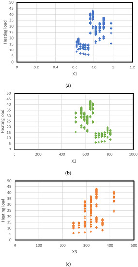
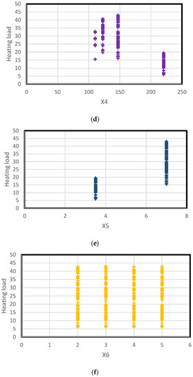
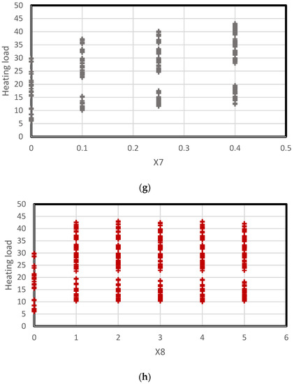
Figure 1.
Box plot of used dataset variations with the heating load. (a) Relative compactness (RC), (b) surface area, (c) wall area, (d) roof area, (e) overall height, (f) orientation, (g) glazing area, (h) glazing area distribution, with the heating load.
3. Methodology
This research examines an ANN with three novel optimizers, MVO, SOSA, and VSA, to test their investigation of how they affect the limits of a typical neural network. These algorithms seek better hyperparameters than those proposed by more conventional learning methods (backpropagation and Levenberg–Marquardt).
3.1. Multilayer Perceptron
Multilayer perceptrons, a type of neural network, have recently been demonstrated to be a viable alternative to conventional statistical methods [74]. Hornik et al. (1989) [75] demonstrated that the MLP could simulate any smooth and measurable function. Despite other methods, the MLP method does not consider data processing. This method can model and teach complex nonlinear functions to generalize correctly using previously unexplored new data. These properties make it a possible alternative to statistical and numerical modeling techniques. The multilayer perceptron has several atmospheric scientific uses, as will be demonstrated.
Figure 2 depicts the predefined connection between the main inputs and output(s) vectors for the multilayer perceptron, a network of fundamentally interconnected neurons or nodes. Each network node’s output signals and weights are derived from a primary activation function or nonlinear transfer. The MLP can only model linear functions if the transfer function is linear. The node’s output can serve as an input for other network-connected nodes for each network-connected node. In light of this, the multilayer perceptron is a feed-forward neural network. There are a variety of structural configurations for multilayer perceptrons, but they all contain layers of neurons. The input layer serves as a conduit for data transfer from the input layer to other network layers. A multilayer perceptron’s input and output vectors can be expressed as single vectors (Figure 2). An MLP structure consists of multiple hidden layers and one output layer. Multilayer perceptron refers to a network in which each node is interconnected in the layers above and below with every other node.
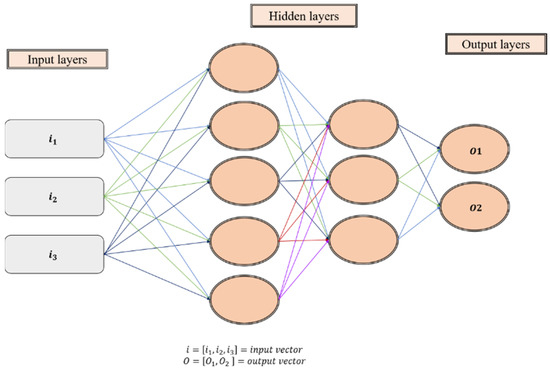
Figure 2.
A two hidden layers multilayer perceptron.
As proven, multilayer perceptrons can estimate any computable function between two sets of input and output vectors by selecting a fine collection of linking weights and transfer functions [75]. A multilayer perceptron is capable of learning new abilities by training. You will require input and output vector-based training data to learn a new algorithm. A multilayer perceptron decides on the network’s weights until the required input-output mapping is reached. It can only acquire knowledge in the presence of an observer. When training an MLP, it is possible that its output for a given input vector may not match the anticipated output. The difference between the actual and desired outputs characterizes error signals. Adjusting the direct networks depending on this error signal during training can help lower the total error of the MLP. A multilayer perceptron can be trained in various methods with several different algorithms. Once trained with adequate training data, the multilayer perceptron can generalize to new, unknown inputs.
3.2. Multi-Verse Optimizer (MVO)
The multi-verse optimizer [76] is known as a growing metaheuristic algorithm that tries to mimic the laws of a multi-verse theory. It is a relatively recent development. Parallel universe theories, including the presence of black, white, and wormholes, were the primary source of inspiration for the design of this optimizer. A population-based stochastic method is employed to determine the global optimum for optimization problems [77]. To update the answers using this method, the probability of wormhole existence (WEP) and the rate of travel (TDR) must first be computed. These parameters determine the frequency and magnitude of solution changes during the optimization process and are formulated as:
The total iterations’ number is T, corresponding to the minimum, b to the maximum, and t to the current iteration.
p indicates the exploitation accuracy. P is the most essential TDR measure. The emphasis on exploitation increases as the value of this choice rises.
The following equation can be used to update the solution positions when WEP and TDR have been calculated:
where is set to be the jth element from the best predefined individual, WEP, TDR are coefficients, lbi and ubi are the lower and upper bounds of the jth element,;; are randomly generated numbers drawn from the interval of [0, 1], represents the jth parameter in ith individual, and . does the roulette wheel selection mechanism to pick the jth element of a solution.
This equation can be used to compute a new solution position and compare it to the most recent best-in-class participant in the WEP. If, a random number in the interval [0, 1], is less than 0.5, then an optimal solution value for the jth dimension requires a solution. By increasing WEP during optimization, MVO increases the use of the most proper solution so far.
3.3. Self-Organizing and Self-Adaptive (SOSA)
Self-organization (SO) parallels the biologically inspired notions of emergence and swarm intelligence very closely. Frequently, in this technique, SO and emergence are conflated. De and Holvoet (2005) [78] examine the phrase’s origins and the difference between the two conceptions. This is known as SO:
SO is an adaptive and dynamic computational process through which systems retain their structure independently of external stimuli [78,79]. However, SO can also refer to the emergence-causing process [80,81]. In addition, ref. [82] differentiates between the terms called strong SO schemes with no explicit central internal or external control and weak SO systems with some central internal control. SO and emergent systems are separate concepts, although they share one characteristic: the absence of direct exterior control. Although the external effect on self-organized systems is studied more thoroughly in directed SO, less attention has been paid to it in the context of unguided SO [83]. In this text, external effect is characterized as either specific or non-specific, with specific influence suggesting straight control on the functional structure or temporal, spatial, or other non-specific impacts indicating that the system determines its response to an external stimulus. Consequently, Prokopenko (2009) [83] defines SO guidance as the potential limiting of the domain or extent of functions/structures, or selecting a subset of the multiple alternatives that the dynamics might take.
According to ref. [78], the main distinction between SO and emergence is that individual entities are informed of the systems planned by global behavior in the former scenario. Consequently, self-organization may be considered a weak kind of emergence. Utilizing feedback loops is a common and straightforward method for achieving SO. Components of the system monitor the state, interpret it according to the expected behavior, and initiate the required actions. This method is also employed by “single entity systems.” This notion is referred to as self-adaptation [84,85]. Self-adaptation happens when a decentralized system composed of several entities adapts to external changes. Self-adaptation within the context of software is set as follows: SA software modifies its behavior in response to modifications within its operating environment. The operating environment refers to everything the software system may see, including human input, sensors and external hardware devices, and programmed instrumentation [86].
3.4. Vortex Search Algorithm (VSA)
Ölmez and Doğan [87] initially developed the vortex pattern generated by the vertical flow of stirred fluids to design the VSA algorithm. As with countless other methods, the algorithm seeks to balance exploratory and exploitative actions. The VSA uses an adaptive step-size-adjustment method to determine the optimal response. Consequently, exploratory behavior is accounted for in the early phases of the VSA, resulting in a better global search capability. In the following, the optimal response is achieved by employing an exploitative strategy around the suggested replies [88].
The vortex is depicted by stacked circles, assuming a set in two dimensions. Given U and L as the current space’s boundaries, Equation (4) produces the starting point . of the outer circle:
Then, several neighbor solutions Ct(s) are generated at random. This production makes use of a Gaussian distribution technique.
where t is the number of cycles and z represents the total number of potential solutions. Let x and Σ be the vector and covariance matrix of the random variable. The multivariate Gaussian distribution is denoted by Equation (6):
The main distribution will be spherical if the off-diagonal elements are uncorrelated and the co-variance matrix values have similar variances (circular for two-dimensional concerns). I, where I is a D × D identity matrix and is the distribution’s variance, Σ may be written as follows:
Using Equation (8), the initial standard deviation of the distribution is computed (). This parameter may correspond to . (which requires significant values) [89]:
As is well known, the essential concept of metaheuristic algorithms for enhancing the final result is to update the obtained answers. During the VSA selection phase, the current is replaced with the most promising alternative. This requires the proposed solution to exist inside the given space. This item is assessed using the Equation (9).
where rand is a random integer with uniform distribution.
The best answer discovered thus far is then applied to the second (or inner) circle’s center. After successively decreasing the effective radius of the current solution, a new group of solutions (C1(s)) is produced close to it. Repetitioning the same approach might yield a more viable answer [89]. Other researches have also described the VSA well [90,91].
4. Results and Discussion
This study analyzes the HL approximation capabilities of three unique neural network upgrades described in Section 1. The algorithms are synthesized using an MLP neural network to accomplish this objective. Each approach uses a unique search strategy to get the optimal computational weights for the MLP (and biases).
As is commonly known, the size and number of neurons contained inside a hidden layer define the MLP’s structure. Therefore, these parameters must initially be modified. Numerous studies have demonstrated that a single hidden layer is excellent at simulating complicated processes [92,93]. However, the hidden neurons’ optimal number was established by trial and error. Among the designs studied, 8 × 6 × 1 demonstrated the most promising performance (where the middling layer contained 1, 2, 3, …, 10 neurons). Figure 2 illustrates the used MLP.
4.1. Accuracy Indicators
Mean absolute error (MAE) as the first used statistical index and root mean square error (RMSE) as the second index was specified for assessing the potential errors in proposed structures. Equations (10) and (11) produce are used for RMSE and MAE. Additionally, Equation (12) defines the coefficient of determination (R2) required to compute the compatibility between the measured and predicted HLs:
and represent the measured and expected HLs, respectively, in these equations. In addition, U represents the number of recordings, whereas Sobserved is the average of the observed HLs.
4.2. Combining the MLP with Hybrid Optimizers
After combining hybrid algorithms with the MLP, three ensembles of MVO-MLP, SOSA-MLP, and SOSA-MLP are constructed. Each costume is supplied with training data to determine the relationship between associated parameters and heating load. One thousand repetitions are assessed for each model’s optimization behavior in order to carry out the optimization. The objective function is represented using the RMSE of each iteration’s findings. In swarm-based optimization algorithms, the population size is a critical variable. Ten distinct population sizes (50, 100, 150, 200, 250, 300, 350, 400, 450, and 500) are evaluated for each proposed model, and the population size results in the lowest MSE chosen as the optimal population size. The MSEs for all calculated iterations are shown in Figure 3. The populations with the lowest RMSE values (0.3540, 8.8064, and 0.2887, respectively) are 300, 4500, and 100 for MVO-MLP, SOSA-MLP, and VSA-MLP, respectively. The SOSA-MLP method, on the other hand, is less sensitive than the other two; the explanation for this may be found in the optimization approaches’ characteristics. Figure 4 also displays the RMSE values achieved for different levels of complexity over all rounds.
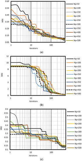
Figure 3.
Model iterations versus the variation of MSE; (a) MVO-MLP, (b) SOSA-MLP, (c) VSA-MLP.
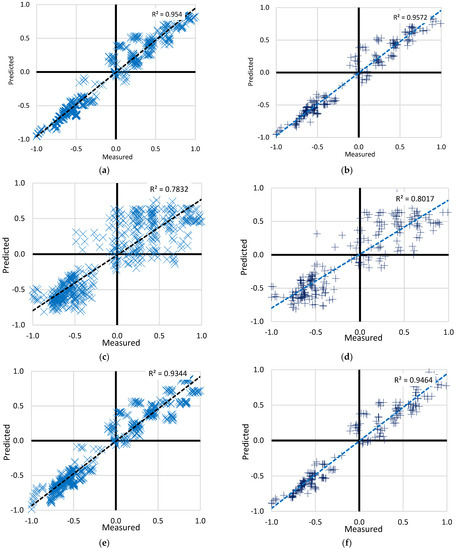
Figure 4.
The accuracy of the best-fit proposed model for the (a) MVO-MLP training dataset, (b) MVO-MLP testing dataset, (c) SOSA-MLP training dataset, (d) SOSA-MLP testing dataset, (e) VSA-MLP training dataset, and (f) VSA-MLP testing dataset.
The value of R2 for three methods of MVO, SOSA, and VSA is (0.977 and 0.978), (0.885 and 0.895), and (0.974 and 0.975) for testing and training phases, respectively. Also, in the case of RMSE, MVO, SOSA, and VSA have the value of (0.117 and 0.110), (0.255 and 0.239), and (0.124 and 0.112) in the training and testing phases, respectively. These results show that the lowest value of RMSE and the highest value of R2 are related to the MVO technique, indicating the best performance of MVO-MLP. According to R2 and RMSE values (Table 1, Table 2, Table 3 and Table 4), the second technique for predicting HL and CL is VSA-MLP, and the last is SOSA-MLP.

Table 1.
The network results for the MVO-MLP.
Table 2.
The network results for the SOSA-MLP.
Table 3.
The network results for the VSA-MLP.
Table 4.
Selection of the best fit structures among the most accurate items of each model.
According to Figure 3, the MVO method has a little more constrained convergence curve than the other methods. This shows that this approach decreases error rates when ANN parameters are altered. As a result, the algorithm’s findings are given to develop a prediction model. Referring to Figure 2, the output of the most recent neuron consists of seven parameters (one bias and six weights). This neuron is nourished by six layers of neurons, each responsible for nine parameters (one bias and eight weights). The network consists of 61 optimized variables with metaheuristic methods.
4.3. Prediction Results
In this section, the reliability of the applied models is assessed by considering both the outputs (i.e., the predicted HLs) to the target values (i.e., the measured HLs). Figure 5 illustrates the outcomes of the training phase by displaying the difference between each pair of output and HL goals. During this phase, the error rate for the MVO-MLP, SOSA-MLP, and VSA-MLP range between [−0.000034913 and 0.11776], [−0.011611 and 0.25559], and [−5.4249 × 10⁻⁵ and 0.12416], respectively. The preceding section indicates that the RMSE values are 0.3540, 8.8064, and 0.2887. In addition, the estimated MAEs of the three models (0.08499, 0.19662, and 0.088861) demonstrate a small degree of training error. Moreover, the computed R2 values indicate that greater than 93% of the objective and output HLs are consistent.
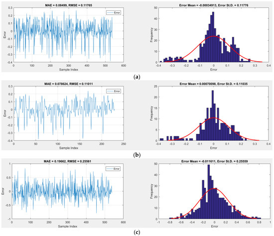
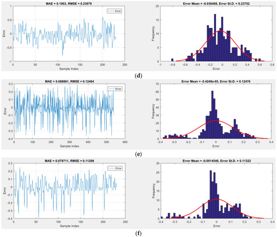
Figure 5.
The error analysis for the best-fit proposed model for the (a) MVO-MLP training dataset, (b) MVO-MLP testing dataset, (c) SOSA-MLP training dataset, (d) SOSA-MLP testing dataset, (e) VSA-MLP training dataset, and (f) VSA-MLP testing dataset.
4.4. Efficiency Comparison
The models with the lowest RMSE (or MAE) and the highest R2 are chosen as the most exact HL predictors, considering the learning and prediction stages. Table 4 displays the accuracy standards that must be satisfied to attain this objective. As demonstrated, the MLP constructed utilizing the MVO’s weights and biases provide the most accurate knowledge of the HL and predicting it. The VSA appears as the second possible optimizer after the MVO. This study’s MVO and VSA algorithms appear to outperform previously proposed models in the training and testing phases. For example, six different MLP network’s hybrids (for instance, based on other hybrid techniques, such as whale optimization algorithm (WOA) [94], ABC [95], PSO [96], the salp swarm algorithm (SSA) [97], wind-driven optimization (WDO) [98], the spotted hyena optimization (SHO) [99], the imperialist competitive algorithm (ICA) [100], GOA [101], the genetic algorithm (GA) [102], and GWO [103]) were utilized to estimate the HL by using the same dataset. This suggests that the objective of developing more effective HL assessment tools has been met.
4.5. Discussion
In several engineering applications, the superiority of intelligent computational techniques over conventional and even solid experimental methods is well acknowledged. In addition to appropriate accuracy, the simplicity of applying these models is a determining factor in their application. In energy-efficiency studies, for instance, forward modeling methodologies (low capabilities for inhabited buildings [104]) and prevalent simulation software may have limitations (low capabilities for occupied buildings [104]). (Different accuracy of simulation [105]). Consequently, like the models reported in this study, indirect evaluative models outperform destructive and expensive methods. This is emphasized further when an optimal strategy is created using metaheuristic methods [106]. In other words, these optimization techniques yield competent ensembles that function optimally.
Realistic applications for the offered approaches may be developed in terms of applicability. Here are two illustrations:
The developed technique can provide an accurate estimate of the needed heating thermal load for an upcoming construction project based on the size and features of the structure [26,107,108]. Engineers and property owners might benefit from the models when developing HVAC systems. Another early-stage support for reconstruction projects is modifying structural design and architecture based on input parameters. Consequently, it is also feasible to examine the effect of each input parameter separately to comprehend the thermal load behavior. Although the trend is not predictable nor regular, the MVO-MLP predicts it precisely. Consequently, this approach may yield approximations of real-world structures that are correct.
Even if there are several benefits to addressing an optimization problem, it is essential to commit the time necessary to discover a global solution. Consequently, achieving a balance between model time economy and precision may impact selecting the most efficient model. Nevertheless, according to the authors, lowering the complexity of the problem space and locating better solutions may be as simple as configuring the hyper-parameters of optimizers correctly and doing feature validity analysis. In contrast, the MVO model was the most precise; this requires establishing the optimal time and accuracy-based method. In projects in which time is not a factor, for instance, it makes sense to choose the most precise technique (regardless of how time-consuming), but in time-sensitive applications, a tolerance for accuracy may be considered in order to find a speedier solution. However, the models’ overall performance was comparable, and it should be emphasized that all versions would be adequate for real-world applications. Table 5 indicates the previous research focused on heating load prediction. Noting that the outcomes were less accurate, either using R2 or RMSE, as those were the hybrid techniques that we employed in the current study.
Table 5.
Studies focused on research on heating load prediction.
5. Conclusions
This study evaluates the MVO, SOSA, and VSA metaheuristic algorithms for analyzing and determining the HL. These methods served as the optimizer for a common neural predictive network simulation. The models predicted the HL based on a total of 768 design scenarios of the heating load. The following conclusions can be drawn from this work:
According to the sensitivity analysis, the MVA-MLP, SOSA-MLP, and VSA-MLP ensembles achieved optimal complexity at corresponding swarm sizes of 300, 500, and 250, respectively. The optimal MVO design required more calculation time than alternative MLP optimization algorithms. In terms of precision (MAEs of 0.08499, 0.19662, and 0.088861), all three ensembles profoundly understood the link between the HL and essential factors. During the testing phase, the measured value for the R2 was 0.978, 0.895, and 0.977 demonstrating that the developed models were successful and had minimal prediction error. The most powerful model was the MVO-MLP, followed by the VSA-MLP and the SOSA-MLP. The MVO-MLP methodology was presented for use in real-world situations, but potential ideas for future projects were also presented in light of the shortcomings of the research, such as data enhancement and future selection, optimizing building characteristics using the model, and comparing the model to improved time-saving methods.
Author Contributions
F.N.: methodology, software, data curation. N.T.: writing—original draft preparation, investigation, validation. M.A.S.: conceptualization, methodology. A.G.: writing—original draft preparation, resources, final draft preparation. M.L.N.: supervision, project administration, funding acquisition. All authors have read and agreed to the published version of the manuscript.
Funding
This research received no external funding.
Data Availability Statement
The data used in this study is freely available on http://archive.ics.uci.edu/ml/datasets/Energy+efficiency (accessed on 15 July 2022).
Conflicts of Interest
The authors declare no conflict of interest.
References
- McQuiston, F.C.; Parker, J.D.; Spitler, J.D. Heating, Ventilating, and Air Conditioning: Analysis and Design; John Wiley & Sons: Hoboken, NJ, USA, 2004. [Google Scholar]
- Ihara, T.; Gustavsen, A.; Jelle, B.P. Effect of facade components on energy efficiency in office buildings. Appl. Energy 2015, 158, 422–432. [Google Scholar] [CrossRef]
- Knight, D.; Roth, S.; Rosen, S.L. Using BIM in HVAC design. Ashrae J. 2010, 52, 24–29. [Google Scholar]
- Ikeda, S.; Ooka, R. Metaheuristic optimization methods for a comprehensive operating schedule of battery, thermal energy storage, and heat source in a building energy system. Appl. Energy 2015, 151, 192–205. [Google Scholar] [CrossRef]
- Sonmez, Y.; Guvenc, U.; Kahraman, H.T.; Yilmaz, C. A comperative study on novel machine learning algorithms for estimation of energy performance of residential buildings. In Proceedings of the 2015 3rd International Istanbul Smart Grid Congress and Fair (ICSG), Istanbul, Turkey, 29–30 April 2015; pp. 1–7. [Google Scholar]
- Lu, N.; Wang, H.; Wang, K.; Liu, Y. Maximum probabilistic and dynamic traffic load effects on short-to-medium span bridges. Comput. Model. Eng. Sci. 2021, 127, 345–360. [Google Scholar] [CrossRef]
- Chen, Y.; Lin, H.; Cao, R.; Zhang, C. Slope stability analysis considering different contributions of shear strength parameters. Int. J. Geomech. 2021, 21, 04020265. [Google Scholar] [CrossRef]
- Zhang, S.-W.; Shang, L.-Y.; Zhou, L.; Lv, Z.-B. Hydrate Deposition Model and Flow Assurance Technology in Gas-Dominant Pipeline Transportation Systems: A Review. Energy Fuels 2022, 36, 1747–1775. [Google Scholar] [CrossRef]
- Liu, E.; Li, D.; Li, W.; Liao, Y.; Qiao, W.; Liu, W.; Azimi, M. Erosion simulation and improvement scheme of separator blowdown system—A case study of Changning national shale gas demonstration area. J. Nat. Gas Sci. Eng. 2021, 88, 103856. [Google Scholar] [CrossRef]
- Peng, S.; Zhang, Y.; Zhao, W.; Liu, E. Analysis of the influence of rectifier blockage on the metering performance during shale gas extraction. Energy Fuels 2021, 35, 2134–2143. [Google Scholar] [CrossRef]
- Zhang, W.; Tang, Z. Numerical modeling of response of CFRP–Concrete interfaces subjected to fatigue loading. J. Compos. Constr. 2021, 25, 04021043. [Google Scholar] [CrossRef]
- Peng, S.; Chen, Q.; Liu, E. The role of computational fluid dynamics tools on investigation of pathogen transmission: Prevention and control. Sci. Total Environ. 2020, 746, 142090. [Google Scholar] [CrossRef]
- Wei, J.; Xie, Z.; Zhang, W.; Luo, X.; Yang, Y.; Chen, B. Experimental study on circular steel tube-confined reinforced UHPC columns under axial loading. Eng. Struct. 2021, 230, 111599. [Google Scholar] [CrossRef]
- Mou, B.; Bai, Y. Experimental investigation on shear behavior of steel beam-to-CFST column connections with irregular panel zone. Eng. Struct. 2018, 168, 487–504. [Google Scholar] [CrossRef]
- Xie, S.-J.; Lin, H.; Chen, Y.-F.; Wang, Y.-X. A new nonlinear empirical strength criterion for rocks under conventional triaxial compression. J. Cent. South Univ. 2021, 28, 1448–1458. [Google Scholar] [CrossRef]
- Ju, B.-K.; Yoo, S.-H.; Baek, C. Economies of Scale in City Gas Sector in Seoul, South Korea: Evidence from an Empirical Investigation. Sustainability 2022, 14, 5371. [Google Scholar] [CrossRef]
- Braspenning, P.J.; Thuijsman, F.; Weijters, A.J.M.M. Artificial Neural Networks: An Introduction to ANN Theory and Practice; Springer Science & Business Media: Berlin, Germany, 1995; Volume 931. [Google Scholar]
- Liu, F.; Zhang, G.; Lu, J. Multisource heterogeneous unsupervised domain adaptation via fuzzy relation neural networks. IEEE Trans. Fuzzy Syst. 2020, 29, 3308–3322. [Google Scholar] [CrossRef]
- Yahya, S.I.; Rezaei, A.; Aghel, B. Forecasting of water thermal conductivity enhancement by adding nano-sized alumina particles. J. Therm. Anal. Calorim. 2021, 145, 1791–1800. [Google Scholar] [CrossRef]
- Peng, S.; Chen, R.; Yu, B.; Xiang, M.; Lin, X.; Liu, E. Daily natural gas load forecasting based on the combination of long short term memory, local mean decomposition, and wavelet threshold denoising algorithm. J. Nat. Gas Sci. Eng. 2021, 95, 104175. [Google Scholar] [CrossRef]
- Seyedashraf, O.; Mehrabi, M.; Akhtari, A.A. Novel approach for dam break flow modeling using computational intelligence. J. Hydrol. 2018, 559, 1028–1038. [Google Scholar] [CrossRef]
- Zhao, Y.; Foong, L.K. Predicting Electrical Power Output of Combined Cycle Power Plants Using a Novel Artificial Neural Network Optimized by Electrostatic Discharge Algorithm. Measurement 2022, 198, 111405. [Google Scholar] [CrossRef]
- Khajehzadeh, M.; Taha, M.R.; Eslami, M. Multi-objective optimisation of retaining walls using hybrid adaptive gravitational search algorithm. Civ. Eng. Environ. Syst. 2014, 31, 229–242. [Google Scholar] [CrossRef]
- Eslami, M.; Neshat, M.; Khalid, S.A. A novel hybrid sine cosine algorithm and pattern search for optimal coordination of power system damping controllers. Sustainability 2022, 14, 541. [Google Scholar] [CrossRef]
- Pinkus, A. Approximation theory of the MLP model in neural networks. Acta Numer. 1999, 8, 143–195. [Google Scholar] [CrossRef]
- Gao, W.; Alsarraf, J.; Moayedi, H.; Shahsavar, A.; Nguyen, H. Comprehensive preference learning and feature validity for designing energy-efficient residential buildings using machine learning paradigms. Appl. Soft Comput. 2019, 84, 105748. [Google Scholar] [CrossRef]
- Ahmad, A.; Ghritlahre, H.K.; Chandrakar, P. Implementation of ANN technique for performance prediction of solar thermal systems: A Comprehensive Review. Trends Renew. Energy 2020, 6, 12–36. [Google Scholar] [CrossRef]
- Liu, T.; Tan, Z.; Xu, C.; Chen, H.; Li, Z. Study on deep reinforcement learning techniques for building energy consumption forecasting. Energy Build. 2020, 208, 109675. [Google Scholar] [CrossRef]
- Guo, Y.; Yang, Y.; Kong, Z.; He, J. Development of Similar Materials for Liquid-Solid Coupling and Its Application in Water Outburst and Mud Outburst Model Test of Deep Tunnel. Geofluids 2022, 2022, 8784398. [Google Scholar] [CrossRef]
- Hornik, K. Approximation capabilities of multilayer feedforward networks. Neural Netw. 1991, 4, 251–257. [Google Scholar] [CrossRef]
- Ren, Z.; Motlagh, O.; Chen, D. A correlation-based model for building ground-coupled heat loss calculation using Artificial Neural Network techniques. J. Build. Perform. Simul. 2020, 13, 48–58. [Google Scholar] [CrossRef]
- Wei, G.; Fan, X.; Xiong, Y.; Lv, C.; Li, S.; Lin, X. Highly disordered VO2 films: Appearance of electronic glass transition and potential for device-level overheat protection. Appl. Phys. Express 2022, 15, 043002. [Google Scholar] [CrossRef]
- Fan, X.; Wei, G.; Lin, X.; Wang, X.; Si, Z.; Zhang, X.; Shao, Q.; Mangin, S.; Fullerton, E.; Jiang, L. Reversible switching of interlayer exchange coupling through atomically thin VO2 via electronic state modulation. Matter 2020, 2, 1582–1593. [Google Scholar] [CrossRef]
- Mohammadhassani, M.; Nezamabadi-pour, H.; Suhatril, M.; Shariati, M. Identification of a suitable ANN architecture in predicting strain in tie section of concrete deep beams. Struct. Eng. Mech. 2013, 46, 853–868. [Google Scholar] [CrossRef]
- Sadeghi, A.; Younes Sinaki, R.; Young, W.A.; Weckman, G.R. An Intelligent Model to Predict Energy Performances of Residential Buildings Based on Deep Neural Networks. Energies 2020, 13, 571. [Google Scholar] [CrossRef]
- Sholahudin, S.; Han, H. Simplified dynamic neural network model to predict heating load of a building using Taguchi method. Energy 2016, 115, 1672–1678. [Google Scholar] [CrossRef]
- Ryu, J.-A.; Chang, S. Data Driven Heating Energy Load Forecast Modeling Enhanced by Nonlinear Autoregressive Exogenous Neural Networks. Int. J. Struct. Civ. Eng. Res. 2019, 8, 246–252. [Google Scholar] [CrossRef]
- Khalil, A.J.; Barhoom, A.M.; Abu-Nasser, B.S.; Musleh, M.M.; Abu-Naser, S.S. Energy efficiency prediction using artificial neural network. Int. J. Acad. Pedagog. Res. 2019, 3, 1–7. [Google Scholar]
- Almutairi, K.; Algarni, S.; Alqahtani, T.; Moayedi, H.; Mosavi, A. A TLBO-Tuned Neural Processor for Predicting Heating Load in Residential Buildings. Sustainability 2022, 14, 5924. [Google Scholar] [CrossRef]
- Cao, B.; Zhao, J.; Liu, X.; Arabas, J.; Tanveer, M.; Singh, A.K.; Lv, Z. Multiobjective evolution of the explainable fuzzy rough neural network with gene expression programming. IEEE Trans. Fuzzy Syst. 2022. [Google Scholar] [CrossRef]
- Adedeji, P.A.; Akinlabi, S.; Madushele, N.; Olatunji, O.O. Hybrid adaptive neuro-fuzzy inference system (ANFIS) for a multi-campus university energy consumption forecast. Int. J. Ambient Energy 2022, 43, 1685–1694. [Google Scholar] [CrossRef]
- Ahmad, T.; Chen, H. Nonlinear autoregressive and random forest approaches to forecasting electricity load for utility energy management systems. Sustain. Cities Soc. 2019, 45, 460–473. [Google Scholar] [CrossRef]
- Namlı, E.; Erdal, H.; Erdal, H.I. Artificial intelligence-based prediction models for energy performance of residential buildings. In Recycling and Reuse Approaches for Better Sustainability; Springer: Berlin/Heidelberg, Germany, 2019; pp. 141–149. [Google Scholar]
- Yepes, V.; Martí, J.V.; García, J. Black hole algorithm for sustainable design of counterfort retaining walls. Sustainability 2020, 12, 2767. [Google Scholar] [CrossRef]
- Jamal, A.; Tauhidur Rahman, M.; Al-Ahmadi, H.M.; Ullah, I.; Zahid, M. Intelligent intersection control for delay optimization: Using meta-heuristic search algorithms. Sustainability 2020, 12, 1896. [Google Scholar] [CrossRef]
- Jitkongchuen, D.; Pacharawongsakda, E. Prediction Heating and cooling loads of building using evolutionary grey wolf algorithms. In Proceedings of the 2019 Joint International Conference on Digital Arts, Media and Technology with ECTI Northern Section Conference on Electrical, Electronics, Computer and Telecommunications Engineering (ECTI DAMT-NCON), Nan, Thailand, 30 January–2 February 2019; pp. 93–97. [Google Scholar]
- Ghahramani, A.; Karvigh, S.A.; Becerik-Gerber, B. HVAC system energy optimization using an adaptive hybrid metaheuristic. Energy Build. 2017, 152, 149–161. [Google Scholar] [CrossRef] [Green Version]
- Foong, L.K.; Zhao, Y.; Bai, C.; Xu, C. Efficient metaheuristic-retrofitted techniques for concrete slump simulation. Smart Struct. Syst. Int. J. 2021, 27, 745–759. [Google Scholar]
- Eslami, M.; Shareef, H.; Mohamed, A. Optimization and coordination of damping controls for optimal oscillations damping in multi-machine power system. Int. Rev. Electr. Eng. 2011, 6, 1984–1993. [Google Scholar]
- Martin, G.L.; Monfet, D.; Nouanegue, H.F.; Lavigne, K.; Sansregret, S. Energy calibration of HVAC sub-system model using sensitivity analysis and meta-heuristic optimization. Energy Build. 2019, 202, 109382. [Google Scholar] [CrossRef]
- Bamdad Masouleh, K. Building Energy Optimisation Using Machine Learning and Metaheuristic Algorithms. Ph.D. Thesis, Queensland University of Technology, Brisbane City, QLD, Australia, 2018. [Google Scholar]
- Moayedi, H.; Mu’azu, M.A.; Foong, L.K. Novel swarm-based approach for predicting the cooling load of residential buildings based on social behavior of elephant herds. Energy Build. 2020, 206, 109579. [Google Scholar] [CrossRef]
- Moayedi, H.; Mosavi, A. Electrical power prediction through a combination of multilayer perceptron with water cycle ant lion and satin bowerbird searching optimizers. Sustainability 2021, 13, 2336. [Google Scholar] [CrossRef]
- Yang, F.; Moayedi, H.; Mosavi, A. Predicting the degree of dissolved oxygen using three types of multi-layer perceptron-based artificial neural networks. Sustainability 2021, 13, 9898. [Google Scholar] [CrossRef]
- Zhao, Y.; Wang, Z. Subset simulation with adaptable intermediate failure probability for robust reliability analysis: An unsupervised learning-based approach. Struct. Multidiscip. Optim. 2022, 65, 172. [Google Scholar] [CrossRef]
- Zhou, G.; Moayedi, H.; Bahiraei, M.; Lyu, Z. Employing artificial bee colony and particle swarm techniques for optimizing a neural network in prediction of heating and cooling loads of residential buildings. J. Clean. Prod. 2020, 254, 120082. [Google Scholar] [CrossRef]
- Nguyen, H.; Moayedi, H.; Jusoh, W.A.W.; Sharifi, A. Proposing a novel predictive technique using M5Rules-PSO model estimating cooling load in energy-efficient building system. Eng. Comput. 2020, 36, 857–866. [Google Scholar] [CrossRef]
- Bui, D.-K.; Nguyen, T.N.; Ngo, T.D.; Nguyen-Xuan, H. An artificial neural network (ANN) expert system enhanced with the electromagnetism-based firefly algorithm (EFA) for predicting the energy consumption in buildings. Energy 2020, 190, 116370. [Google Scholar] [CrossRef]
- Moayedi, H.; Nguyen, H.; Kok Foong, L. Nonlinear evolutionary swarm intelligence of grasshopper optimization algorithm and gray wolf optimization for weight adjustment of neural network. Eng. Comput. 2021, 37, 1265–1275. [Google Scholar] [CrossRef]
- Moayedi, H.; Bui, D.T.; Dounis, A.; Lyu, Z.; Foong, L.K. Predicting heating load in energy-efficient buildings through machine learning techniques. Appl. Sci. 2019, 9, 4338. [Google Scholar] [CrossRef] [Green Version]
- Moayedi, H.; Mehrabi, M.; Bui, D.T.; Pradhan, B.; Foong, L.K. Fuzzy-metaheuristic ensembles for spatial assessment of forest fire susceptibility. J. Environ. Manag. 2020, 260, 109867. [Google Scholar] [CrossRef] [PubMed]
- Zhao, Y.; Hu, H.; Song, C.; Wang, Z. Predicting compressive strength of manufactured-sand concrete using conventional and metaheuristic-tuned artificial neural network. Measurement 2022, 194, 110993. [Google Scholar] [CrossRef]
- Zhao, Y.; Yan, Q.; Yang, Z. A Novel Artificial Bee Colony Algorithm for Structural Damage Detection. Adv. Civ. Eng. 2020, 2020, 3743089. [Google Scholar] [CrossRef]
- Khajehzadeh, M.; Taha, M.R.; Eslami, M. A new hybrid firefly algorithm for foundation optimization. Natl. Acad. Sci. Lett. 2013, 36, 279–288. [Google Scholar] [CrossRef]
- Zhao, Y.H.; Joseph, A.; Zhang, Z.W. Deterministic Snap-Through Buckling and Energy Trapping in Axially-Loaded Notched Strips for Compliant Building Blocks. Smart Mater. Struct. 2020, 29, 02LT03. [Google Scholar] [CrossRef]
- Khajehzadeh, M.; Keawsawasvong, S.; Nehdi, M.L. Effective hybrid soft computing approach for optimum design of shallow foundations. Sustainability 2022, 14, 1847. [Google Scholar] [CrossRef]
- Khajehzadeh, M.; Taha, M.R.; Eslami, M. Multi-objective optimization of foundation using global-local gravitational search algorithm. Struct. Eng. Mech. 2014, 50, 257–273. [Google Scholar] [CrossRef]
- Zhao, Y.; Hu, H.; Bai, L. Fragility Analyses of Bridge Structures Using the Logarithmic Piecewise Function-Based Probabilistic Seismic Demand Model. Sustainability 2021, 13, 7814. [Google Scholar] [CrossRef]
- Eslami, M.; Shareef, H.; Mohamed, A.; Khajehzadeh, M. Damping controller design for power system oscillations using hybrid GA-SQP. Int. Rev. Electr. Eng. 2011, 6, 888–896. [Google Scholar]
- Khajehzadeh, M.; Taha, M.R.; Keawsawasvong, S.; Mirzaei, H.; Jebeli, M. An effective artificial intelligence approach for slope stability evaluation. IEEE Access 2022, 10, 5660–5671. [Google Scholar] [CrossRef]
- Mehrabi, M.; Moayedi, H. Landslide susceptibility mapping using artificial neural network tuned by metaheuristic algorithms. Environ. Earth Sci. 2021, 80, 804. [Google Scholar] [CrossRef]
- Zhao, Y.; Moayedi, H.; Bahiraei, M.; Kok Foong, L. Employing TLBO and SCE for optimal prediction of the compressive strength of concrete. Smart Struct. Syst. 2020, 26, 753–763. [Google Scholar] [CrossRef]
- Tsanas, A.; Xifara, A. Accurate quantitative estimation of energy performance of residential buildings using statistical machine learning tools. Energy Build. 2012, 49, 560–567. [Google Scholar] [CrossRef]
- Robert, J.S. Pattern Recognition: Statistical, Structural and Neural Approaches; Wiley India Pvt. Limited: Noida, India, 1992; ISBN 8126513705. [Google Scholar]
- Hornik, K.; Stinchcombe, M.; White, H. Multilayer feedforward networks are universal approximators. Neural Netw. 1989, 2, 359–366. [Google Scholar] [CrossRef]
- Mirjalili, S.; Mirjalili, S.M.; Hatamlou, A. Multi-verse optimizer: A nature-inspired algorithm for global optimization. Neural Comput. Appl. 2016, 27, 495–513. [Google Scholar] [CrossRef]
- Zhao, Y.; Zhong, X.; Foong, L.K. Predicting the splitting tensile strength of concrete using an equilibrium optimization model. Steel Compos. Struct. Int. J. 2021, 39, 81–93. [Google Scholar]
- Wolf, T.D.; Holvoet, T. Emergence versus self-organisation: Different concepts but promising when combined. In Proceedings of the International Workshop on Engineering Self-Organising Applications; ESOA: Berlin/Heidelberg, Germany, 2005; pp. 1–15. [Google Scholar]
- Wang, J.; Tian, J.; Zhang, X.; Yang, B.; Liu, S.; Yin, L.; Zheng, W. Control of Time Delay Force Feedback Teleoperation System With Finite Time Convergence. Front. Neurorobot. 2022, 16, 877069. [Google Scholar] [CrossRef] [PubMed]
- Goldstein, J. Emergence as a construct: History and issues. Emergence 1999, 1, 49–72. [Google Scholar] [CrossRef]
- Noël, V.; Zambonelli, F. Methodological guidelines for engineering self-organization and emergence. In Software Engineering for Collective Autonomic Systems; Springer: Berlin/Heidelberg, Germany, 2015; pp. 355–378. [Google Scholar]
- Serugendo, G.D.M.; Gleizes, M.-P.; Karageorgos, A. Self-organization in multi-agent systems. Knowl. Eng. Rev. 2005, 20, 165–189. [Google Scholar] [CrossRef]
- Prokopenko, M. Guided Self-Organization; Taylor & Francis: London, UK, 2009. [Google Scholar]
- Brun, Y.; Marzo Serugendo, G.D.; Gacek, C.; Giese, H.; Kienle, H.; Litoiu, M.; Müller, H.; Pezzè, M.; Shaw, M. Engineering self-adaptive systems through feedback loops. In Software Engineering for Self-Adaptive Systems; Springer: Berlin/Heidelberg, Germany, 2009; pp. 48–70. [Google Scholar]
- Lemos, R.d.; Giese, H.; Müller, H.A.; Shaw, M.; Andersson, J.; Litoiu, M.; Schmerl, B.; Tamura, G.; Villegas, N.M.; Vogel, T. Software engineering for self-adaptive systems: A second research roadmap. In Software Engineering for Self-Adaptive Systems II; Springer: Berlin/Heidelberg, Germany, 2013; pp. 1–32. [Google Scholar]
- Oreizy, P.; Gorlick, M.M.; Taylor, R.N.; Heimhigner, D.; Johnson, G.; Medvidovic, N.; Quilici, A.; Rosenblum, D.S.; Wolf, A.L. An architecture-based approach to self-adaptive software. IEEE Intell. Syst. Appl. 1999, 14, 54–62. [Google Scholar] [CrossRef]
- Doğan, B.; Ölmez, T. A new metaheuristic for numerical function optimization: Vortex Search algorithm. Inf. Sci. 2015, 293, 125–145. [Google Scholar] [CrossRef]
- Doğan, B.; Ölmez, T. Vortex search algorithm for the analog active filter component selection problem. AEU-Int. J. Electron. Commun. 2015, 69, 1243–1253. [Google Scholar] [CrossRef]
- Dogan, B.; Ölmez, T. Modified off-lattice AB model for protein folding problem using the vortex search algorithm. Int. J. Mach. Learn. Comput. 2015, 5, 329. [Google Scholar] [CrossRef]
- Altintasi, C.; Aydin, O.; Taplamacioglu, M.C.; Salor, O. Power system harmonic and interharmonic estimation using Vortex Search Algorithm. Electr. Power Syst. Res. 2020, 182, 106187. [Google Scholar] [CrossRef]
- Qyyum, M.A.; Yasin, M.; Nawaz, A.; He, T.; Ali, W.; Haider, J.; Qadeer, K.; Nizami, A.-S.; Moustakas, K.; Lee, M. Single-solution-based vortex search strategy for optimal design of offshore and onshore natural gas liquefaction processes. Energies 2020, 13, 1732. [Google Scholar] [CrossRef]
- Nguyen, H.; Mehrabi, M.; Kalantar, B.; Moayedi, H.; Abdullahi, M.a.M. Potential of hybrid evolutionary approaches for assessment of geo-hazard landslide susceptibility mapping. Geomat. Nat. Hazards Risk 2019, 10, 1667–1693. [Google Scholar] [CrossRef]
- Mehrabi, M. Landslide susceptibility zonation using statistical and machine learning approaches in Northern Lecco, Italy. Nat. Hazards 2022, 111, 901–937. [Google Scholar] [CrossRef]
- Mirjalili, S.; Lewis, A. The whale optimization algorithm. Adv. Eng. Softw. 2016, 95, 51–67. [Google Scholar] [CrossRef]
- Karaboga, D. An Idea Based on Honey Bee Swarm for Numerical Optimization; Technical Report-tr06; Erciyes University, Engineering Faculty, Computer: Kayseri, Turkey, 2005. [Google Scholar]
- Kennedy, J.; Eberhart, R. Particle swarm optimization. In Proceedings of the ICNN’5-International Conference on Neural Networks, Perth, Australia, 27 November 1995; pp. 1942–1948. [Google Scholar]
- Mirjalili, S.; Gandomi, A.H.; Mirjalili, S.Z.; Saremi, S.; Faris, H.; Mirjalili, S.M. Salp Swarm Algorithm: A bio-inspired optimizer for engineering design problems. Adv. Eng. Softw. 2017, 114, 163–191. [Google Scholar] [CrossRef]
- Bayraktar, Z.; Komurcu, M.; Werner, D.H. Wind Driven Optimization (WDO): A novel nature-inspired optimization algorithm and its application to electromagnetics. In Proceedings of the 2010 IEEE Antennas and Propagation Society International Symposium, Toronto, ON, Canada, 11–17 July 2010; pp. 1–4. [Google Scholar]
- Dhiman, G.; Kumar, V. Multi-objective spotted hyena optimizer: A multi-objective optimization algorithm for engineering problems. Knowl.-Based Syst. 2018, 150, 175–197. [Google Scholar] [CrossRef]
- Atashpaz-Gargari, E.; Lucas, C. Imperialist competitive algorithm: An algorithm for optimization inspired by imperialistic competition. In Proceedings of the 2007 IEEE Congress on Evolutionary Computation, Singapore, 25–28 September 2007; pp. 4661–4667. [Google Scholar]
- Saremi, S.; Mirjalili, S.; Lewis, A. Grasshopper optimisation algorithm: Theory and application. Adv. Eng. Softw. 2017, 105, 30–47. [Google Scholar] [CrossRef]
- Holland, J.H. Genetic algorithms. Sci. Am. 1992, 267, 66–73. [Google Scholar] [CrossRef]
- Mirjalili, S.; Mirjalili, S.M.; Lewis, A. Grey wolf optimizer. Adv. Eng. Softw. 2014, 69, 46–61. [Google Scholar] [CrossRef]
- Park, J.; Lee, S.J.; Kim, K.H.; Kwon, K.W.; Jeong, J.-W. Estimating thermal performance and energy saving potential of residential buildings using utility bills. Energy Build. 2016, 110, 23–30. [Google Scholar] [CrossRef]
- Yezioro, A.; Dong, B.; Leite, F. An applied artificial intelligence approach towards assessing building performance simulation tools. Energy Build. 2008, 40, 612–620. [Google Scholar] [CrossRef]
- Gong, X.; Wang, L.; Mou, Y.; Wang, H.; Wei, X.; Zheng, W.; Yin, L. Improved Four-channel PBTDPA control strategy using force feedback bilateral teleoperation system. Int. J. Control Autom. Syst. 2022, 20, 1002–1017. [Google Scholar] [CrossRef]
- Bui, X.-N.; Moayedi, H.; Rashid, A.S.A. Developing a predictive method based on optimized M5Rules–GA predicting heating load of an energy-efficient building system. Eng. Comput. 2020, 36, 931–940. [Google Scholar] [CrossRef]
- Fang, J.; Kong, G.; Yang, Q. Group Performance of Energy Piles under Cyclic and Variable Thermal Loading. J. Geotech. Geoenviron. Eng. 2022, 148, 04022060. [Google Scholar] [CrossRef]
- Tien Bui, D.; Moayedi, H.; Anastasios, D.; Kok Foong, L. Predicting heating and cooling loads in energy-efficient buildings using two hybrid intelligent models. Appl. Sci. 2019, 9, 3543. [Google Scholar] [CrossRef] [Green Version]
Publisher’s Note: MDPI stays neutral with regard to jurisdictional claims in published maps and institutional affiliations. |
© 2022 by the authors. Licensee MDPI, Basel, Switzerland. This article is an open access article distributed under the terms and conditions of the Creative Commons Attribution (CC BY) license (https://creativecommons.org/licenses/by/4.0/).