1. Introduction
Asset management is the method by which facility managers plan and care for built infrastructure and facilities. Both public and private entities are responsible for managing asset portfolios over their life cycles. This is a challenging task, especially for large agencies such as universities, hospitals, supply-chain companies, and municipalities. Ultimately, all organizations with built infrastructure portfolios face the same asset management problem [
1], with America’s infrastructure rated a D+ [
2].
Whether accounted for in facility conditions or dollars, deferred maintenance is growing in attention because it has been growing in deferment in the US since the 1930s [
3]. For example, the United States Department of Defense (DoD) was authorized
$26.7 billion in fiscal year 2020 to construct, repair, alter, maintain, and modernize its 585,000 facilities and associated infrastructure [
4]. Despite this considerable funding that results from the DoD’s annual budget of 1.2% of these assets’ replacement values [
5], there remains an estimated
$116 billion maintenance project backlog [
6]. The DoD manages one of the largest global facility portfolios, but unfortunately the DoD is not an anomaly when it comes to foregone maintenance [
3]. Globally, there is a backlog of facility and infrastructure maintenance, and DoD asset management policy has created one of the largest and most uniform international facility databases to date.
Asset management requires the creation of a comprehensive infrastructure inventory, which makes prioritizing essential repairs and replacement projects, in addition to planning a long-term capital budget, efficient for policymakers and asset owners [
7]. Since the condition of assets is not static, plans must be routinely updated to ensure asset strategies and management decisions are in sync with degradation. Current degradation models suggest that infrastructure assets age with time or experience age-based obsolescence [
8], but several distinct factors cause degradation. Degradation directly results from exogenous influences acting on infrastructure or assets, and roofing systems are among the most exposed built assets. Research shows that heat aging, roof traffic, roof slope, and annual maintenance [
9] are significant degradation factors in addition to extreme weather events [
10], such as hail damage or heat stress from high-temperature extremes and solar radiance [
11].
Additionally, time appears to influence roof service life [
12]. While the correlation between roofing types and specific degradation factors is being drawn, the research gap is still quite broad when trying to use these factors to predict roofing degradation. For this reason, life-cycle analysis is typically the most impactful justification to support roofing research and project decisions [
13]. However, when an analysis of five types of service-life software was conducted, the variation of predictions for the service life of three different roof systems (built-up, thermoplastic or single-ply, and vegetated) within these models was extreme [
14]. The tension between using broad life-cycle predictions and factor-specific degradation models leads current research to employ data gathered by asset management databases.
Asset management methodologies have been in place for decades for several infrastructure domains, including roads and pavements, railroads, bridges, and distribution pipelines [
15]. Over the past ten years, industry leaders have also begun to use Enterprise Asset Management (EAM) systems to collect and standardize asset condition data across their diverse portfolio of facility assets, such as roofs [
8]. Two of these systems are the BUILDER Sustainment Management System (SMS) [
15] and BELCAM [
16]. While the software differs somewhat technically, both concept models start with population trends and adjust those trends using observed condition inspection data. This approach results in shaping or scaling population expectations instead of a tailored prediction for assets with a similar inspection history. Decision makers use these systems’ data to predict asset degradation and expected service life, enabling prioritized maintenance, repair, and renovation actions to reduce asset life-cycle costs and achieve organizational objectives.
This data-driven approach to asset management has been increasing in popularity, and it is also growing in use as a management tool as the amount of data collected for facilities and infrastructure continues to grow. Converting these existing data sets into prediction models to forecast future asset conditions requires quantity, quality, and management decision threshold hurdles to be overcome. In contrast to early Gompertz, Richard, or Morgan–Mercer–Flodin models [
17], current models use statistical methods such as the Weibull probability distribution function [
18] to fit a continuous function to asset data and make condition predictions as a function of age, or the Discrete Markov process [
19] to predict the probability of a component being in a particular condition state at a particular time step. These approaches focus on population life-cycle expectations to make future probabilistic life-cycle predictions of individual assets. The standard industry practice of viewing assets in terms of service-life ranges or life cycles [
9] results in large prediction ranges, thus labeling the performance of individual assets from year to year a stochastic phenomenon [
14].
A holistic data-driven approach could instead be applied to predict asset-specific conditions throughout its life instead of just focusing on an end-of-life expectation for the population overall. The BUILDER SMS assessment process discussed above records the condition of individual assets in quantitative form as a Condition Index (CI) score [
20], enabling asset performance to be tracked over time. This quantitative indexing of asset conditions equips decision makers to manage asset portfolios in a prioritized fashion [
21]. This same method of indexing asset-specific conditions over time can be coupled with other attribute data in the asset management database to develop a precise, data-driven stepwise method by extracting groups of assets with similar performance behaviors at times of inspection and using the characteristics of those groups to make future condition predictions. Leveraging this comprehensive data set as a tool to improve both short- and long-term prediction models enables better management decisions and reduces the risk of premature asset failures and financially crippling expenses [
22].
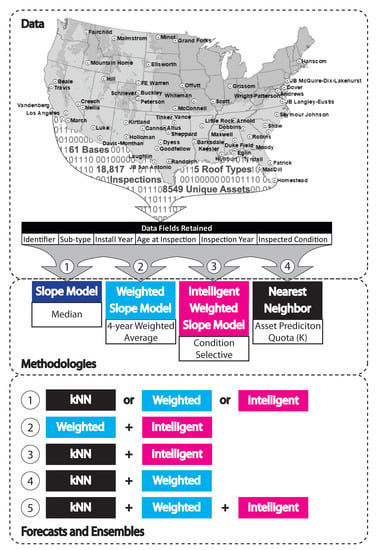
Despite the significant contributions of the aforementioned studies and SMS, current asset prediction methods still only produce broad life-cycle expectations from population data or failure probabilities instead of asset-specific condition expectations. Industry tends to view asset condition prediction from an end-of-life perspective, which is meant to inform replacement planning. However, this leaves large gaps in understanding an asset’s performance over its lifespan, which translates to poor maintenance and repair management planning. For this reason, research into different predictive model types and their strengths and weaknesses is imperative to provide managers skillful predictions at all points along the asset life cycle. Data-driven forecasts can be developed to fill this gap. Four new model types will be discussed and compared as ways to convert asset data into degradation predictions using (1) Slope, (2) Weighted Slope, (3) Condition-Intelligent Weighted Slope, and (4) Nearest Neighbor approaches. The methods for creating each of the model types will be explained, and the prediction strengths of each type will be discussed along with insights on how to employ them singularly or as ensemble tools for making management decisions.
As an illustration of each model approach’s efficacy, this research uses Air Force roof data from 61 unique US locations. Both model prediction values and BUILDER SMS prediction values [
23] are compared with observation data to quantify degradation prediction improvements for each model. Roofing systems were selected over other assets because the average expected life cycle is 20–30 years, as opposed to other building systems, which have an expected life cycle that is typically 2–3 times longer [
13]. Selecting assets with a shorter life cycle requires a smaller temporal data range for calibration and validation. Given that BUILDER data has only been collected for 11 years, results for longer-lived assets would be speculative. Stated alternatively, the sheer number of facilities operated by the United States Air Force (USAF) means that the number of roofs tracked across various segments of their life cycle will provide a statistically significant sample with which to perform this analysis.
2. Data and Case Study
BUILDER SMS inspection data were gathered from 61 unique, contiguous USAF installations and used in this analysis to provide a representative sample of variations in manufacturer, climate, maintenance, and other conditions present across the enterprise. The data include time-based Condition Index (CI) records for assets installed between 1985 and July 2020. Roof system data was selected for this case study because roofing subtypes have a range of service-life expectancies between 20 and 50 years, which helps prove this research’s applicability to assets of differing service-life expectancies. Roofing (B30) data were collected utilizing BUILDER SMS reports titled AF QC 06, which give a comprehensive catalog of assets down to the system sub-type level [
24]. At the system sub-type level, an individual asset has multiple unique inspections over its service life. These inspection values are used to filter the data for quality purposes before employing the data.
2.1. Data Quality
SMS data quality and quantity must first be assessed to create a tailored model. While the USAF employs standardized maintenance plans, routine inspections, and uniform condition metrics, data quality and consistency vary across locations based on the subjectivity of technician ratings of the assets and projects that improve an asset’s condition. This is why stringent pre-processing and filtering of the data was employed. Additionally, data quantity increases with the number of locations included in the study and as inspections occur over time. The USAF data provide a unique opportunity to maximize both the quantity and uniform quality of asset data simultaneously.
2.1.1. Filtering Hierarchy
The data were filtered to remove all roof subtypes other than Built-Up Roofing (BUR), Modified Bitumen Roofing (MOD), Single-Ply (SP), Shingle (SH), and Standing Seam Metal (SSM) roof-types. The roofing service life of these five roofing types are known to be different, so they were selected for comparison. All other roofing types were not analyzed in this study.
2.1.2. Cleaning Hierarchy
The data cleaning process employed is listed below and quantified in
Table 1.
Remove repaired assets: If the Observed Condition Index (OCI) of the asset improved from one inspection to the next (OCI2–OCI1 ≥ +1), this asset was removed. Note: Component Section Condition Index (CSCI) was used, but for simplified communication, these values are referred to as “CI” in this paper.
Remove replaced assets: If the original construction date changed from one rating period to the next, this asset was removed.
If an asset had less than a perfect score (100 = CI) at age zero, this asset was removed because assets not in perfect condition when installed contain install defects.
If an asset had a score of zero (0 = CI), the asset was removed.
Component Specifics
The data fields retained for analysis of the assets were Unique Asset Identifier, System Sub-Type, Asset Install/Construction Year, Asset Age at time of Inspection, Year of Inspection, and Condition at Inspection.
Roofs: 870 Built-Up Roofing (BUR), 461 Modified Bitumen Roofing (MOD), 525 Single-Ply (SP), 476 Shingle (SH), and 1179 Standing Seam Metal (SSM) roof-types were selected as the components for comparison. The roofing service life of these five roofing types are known to be different, so they were analyzed separately. All other roofing types were not analyzed in this study.
2.2. Development of New Variables/Data Explained
Initial analysis of the data revealed that minor post-processing was required to utilize the data for model building purposes. These data processing steps are described below.
2.2.1. Calculating Age
The temporal scale provided was converted from a relative date to an absolute asset age, allowing assets of the same age with different installation dates to be compared.
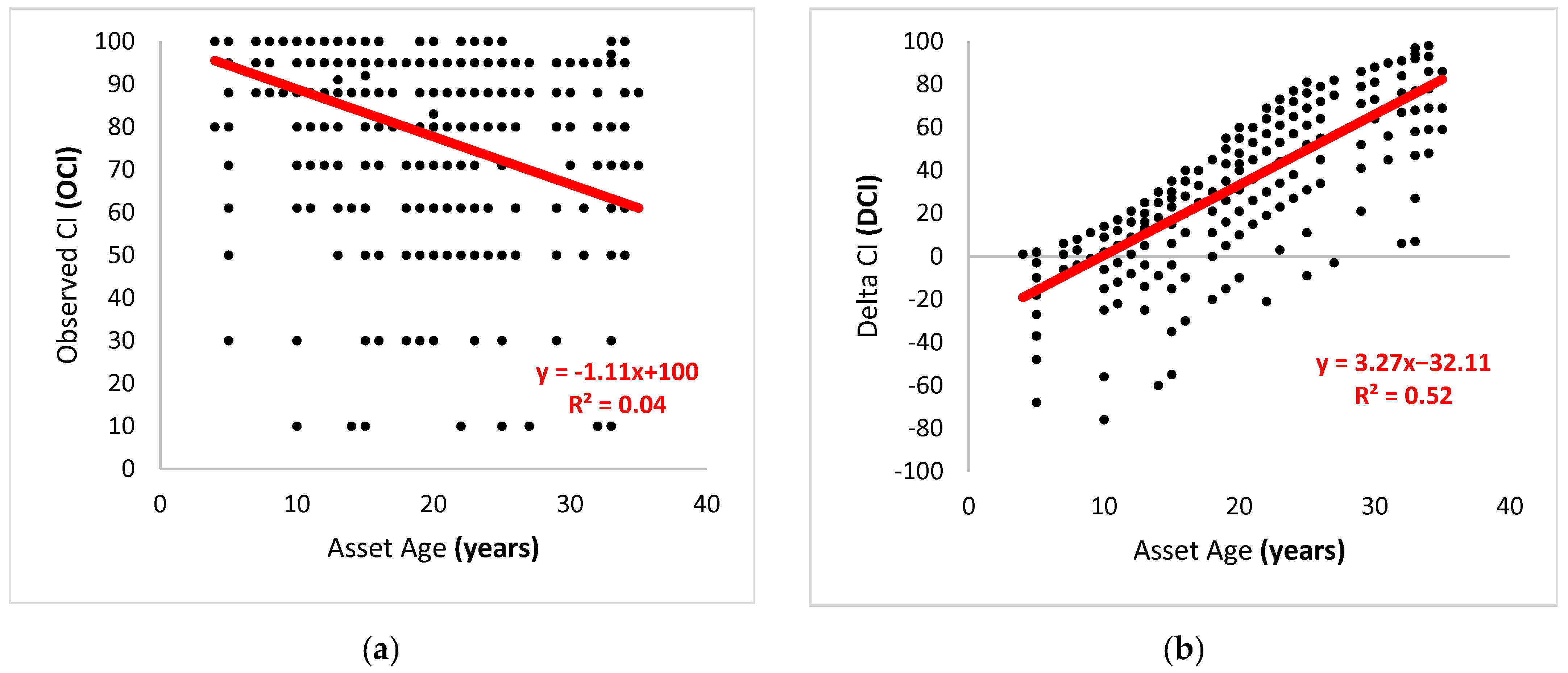
2.2.2. Delta Condition versus Condition
Raw data from BUILDER was captured in OCI, while BUILDER predictions were assigned an Expected CI (ECI). The calculation for BUILDER SMS ECI values was an output of the age-dependent Weibull function it employed. When looking at the correlation between age and OCI (
Figure 1a), the R
2 value was very low, suggesting that they were not inherently related. However, an analysis of the residuals or Delta Condition Index (DCI), calculated by subtracting Expected CI (ECI) from the Observed CI (OCI), revealed a strong relationship in the data. Although the signal was strong, plotting the age versus DCI (
Figure 1b) showed that the data range was widely spread across the possible outcomes. The increase in the R
2 values between the two figures is noticeable, although the spread, or range, of the data remains at around 100 CI points in both figures.
2.3. Limitations
The filtering process ultimately reduced data quantity, while maximizing data quality remained the same. Only 11% of the original data were retained. This is likely because as assets age, they are more likely to have a repair, replacement, or maintenance action, which ultimately removed those assets from inclusion in the analysis. The quantity trade-off is one that should increase confidence in the results of this research. However, as the number of data subsets that were used increased, each subset’s size decreased.
For this reason, more data is always more powerful and will produce different results. While this research’s methods are applicable to multiple data samples, the results and discussion are applicable to this specific sample only. Another limitation of the data is that USAF BUILDER guidance requires each asset be inspected at least once every five years, although more frequent inspections are encouraged. Inspection intervals, inspector, and other intangible factors vary across the assets. Additionally, while older assets are required to have more inspections, many assets have annual or semi-annual inspections performed for warranty purposes. The frequency of inspections ultimately results in differing data resolution between assets. While this research aimed to synthesize these differences by increasing data quantity, these differences were not studied in depth.
3. Materials and Methods
An iterative, data-driven methodology resulted in the production of four asset degradation prediction models. The following methodology will explain the models that build from the most simplistic to the most rigorous. There are several reasons to develop multiple models instead of relying on a singular model. First, researchers should seek to create the least complicated tool that provides the level of service necessary to make the decisions they want. In this case, predictions need to be accurate throughout the asset’s life cycle to make better maintenance and repair decisions. Secondly, the iterative approach creates models that could be useful for other data and assets. Even if a particular model is not useful in this study, alternative conditions could prove the model more useful. Finally, the creation of more than one model allows for trade-offs and ensembles, which often provide better results than a single model can achieve on its own. Ultimately, more than one model can be coupled to provide the best results. The iterative methodology presented below provides a robust use of the data to satisfy both short and long-term decision needs.
There are several commonalities between the model types, such as initial search space and stepwise computation. Search space constraints limit the initial data that the model explores to obtain input variables before applying mathematical computation, and it can be categorized by age (x) or condition (y). Model types are developed using different initial search spaces and mathematical treatment of the data once selected as input variables (
Table 2). Stepwise computation is used to convert discrete condition and age outcomes into a complete model by selectively interpolating data based on groups of similar assets. This process is different from fitting a continuous function to a data set because the focus of stepwise computation is incrementally slope-based, which results in the data and model being much closer aligned. All model iterations employ stepwise computation and analysis of the case study data. The model overview in
Table 2 shows the search space, input variable, and general description of the mathematical operation(s) applied to convert the input data into a prediction value.
3.1. Slope Model (SM)
Methods: The first-generation model is the Slope Model (SM). The prediction at any age (x) is the median value of all asset inspections (OCI) at that discrete time step.
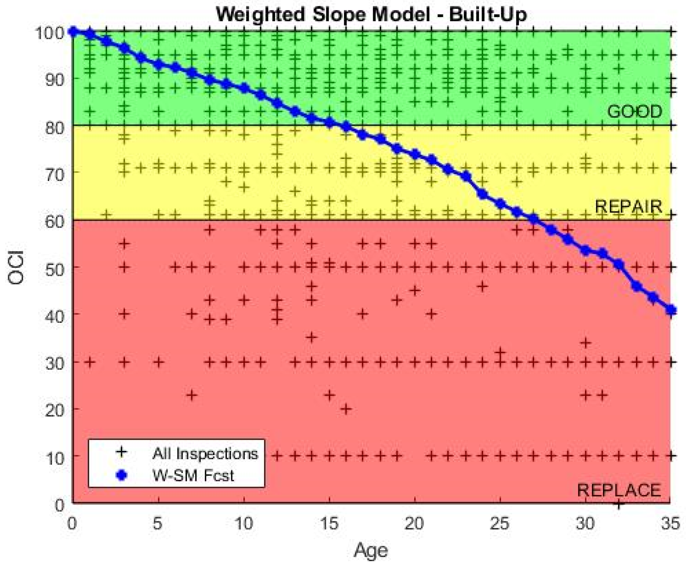
3.2. Weighted-Slope Model (W-SM)
Methods: The second-generation model is the Weighted-Slope Model (W-SM) shown in
Figure 2, which focuses on individual asset performance over a four-year period instead of performance at a single discrete age. The W-SM uses a four-year, forward-looking search of the data set to calculate a weighted average ECI for a single target asset at age (
) to predict the next year’s (
) condition, as shown in Equations (1) and (2).
where:
= the Expected Condition Index (ECI) produced by the model for the next year;
= the Observed Condition Index (OCI) of the asset in question at its last inspection;
= the total number of years past the current inspection;
= the out-year index between zero and ;
= the proximity weighted value assigned to each out-year, where the weight assigned is greater than or equal to zero and decreases as the out-year increases, and all weight values sum to one; and
= the average change in condition of assets from each out-year.
The model is a proximal weighted average of the collective assets’ condition averages at years past the observed condition of the asset in question. For example, if , which is used in the research, the search space is 4 years past the inspection of an asset at . Weight values are , , , and respectively, for out-years 1, 2, 3, and 4. Thus, any asset at age = t is expected to degrade in condition at the same rate, or slope, as the model at age = t.
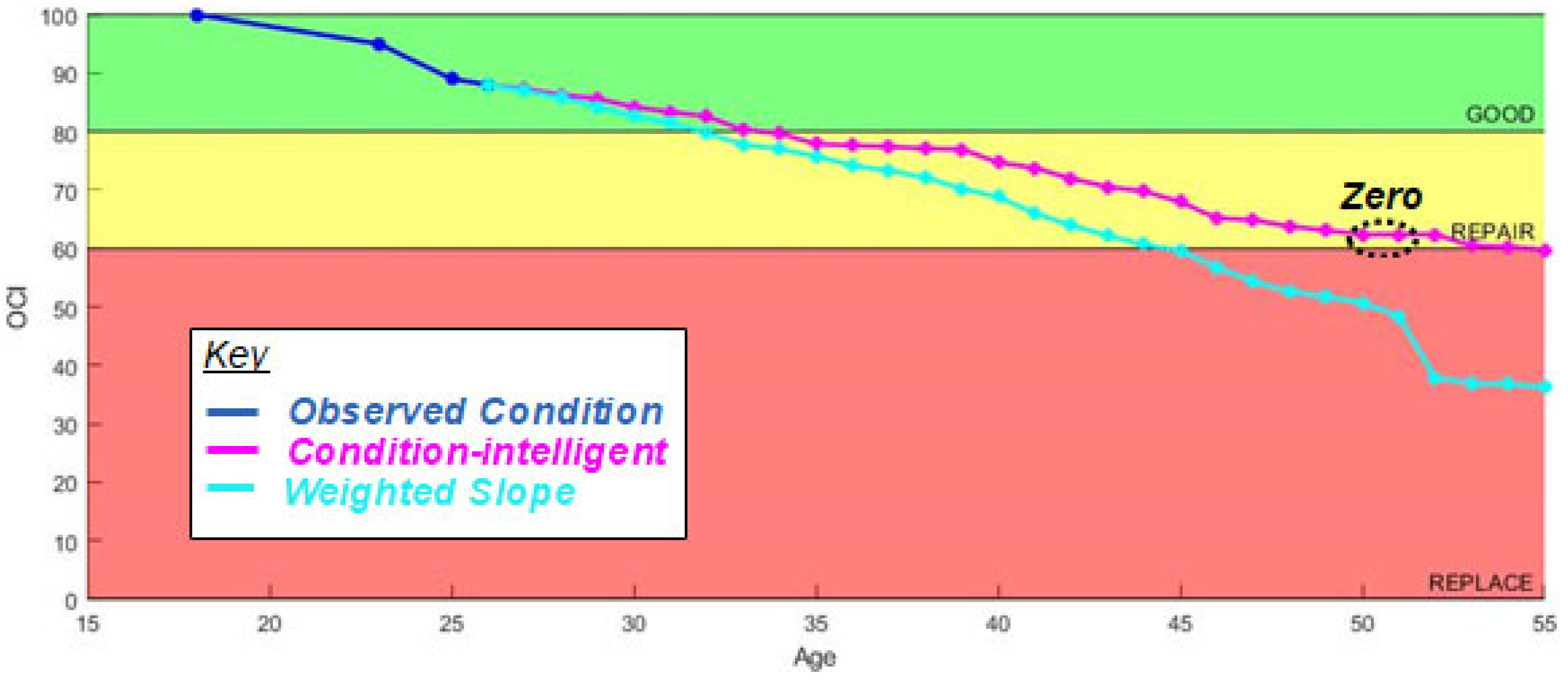
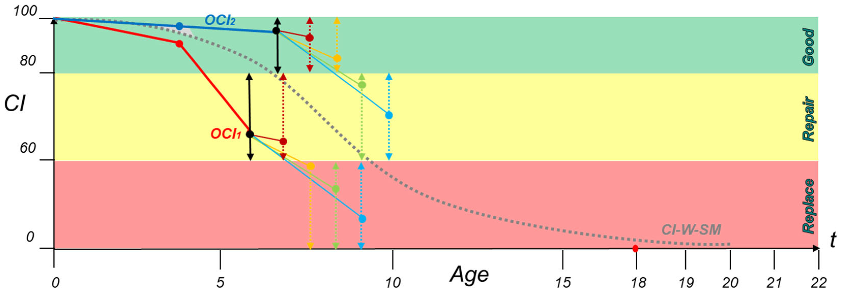
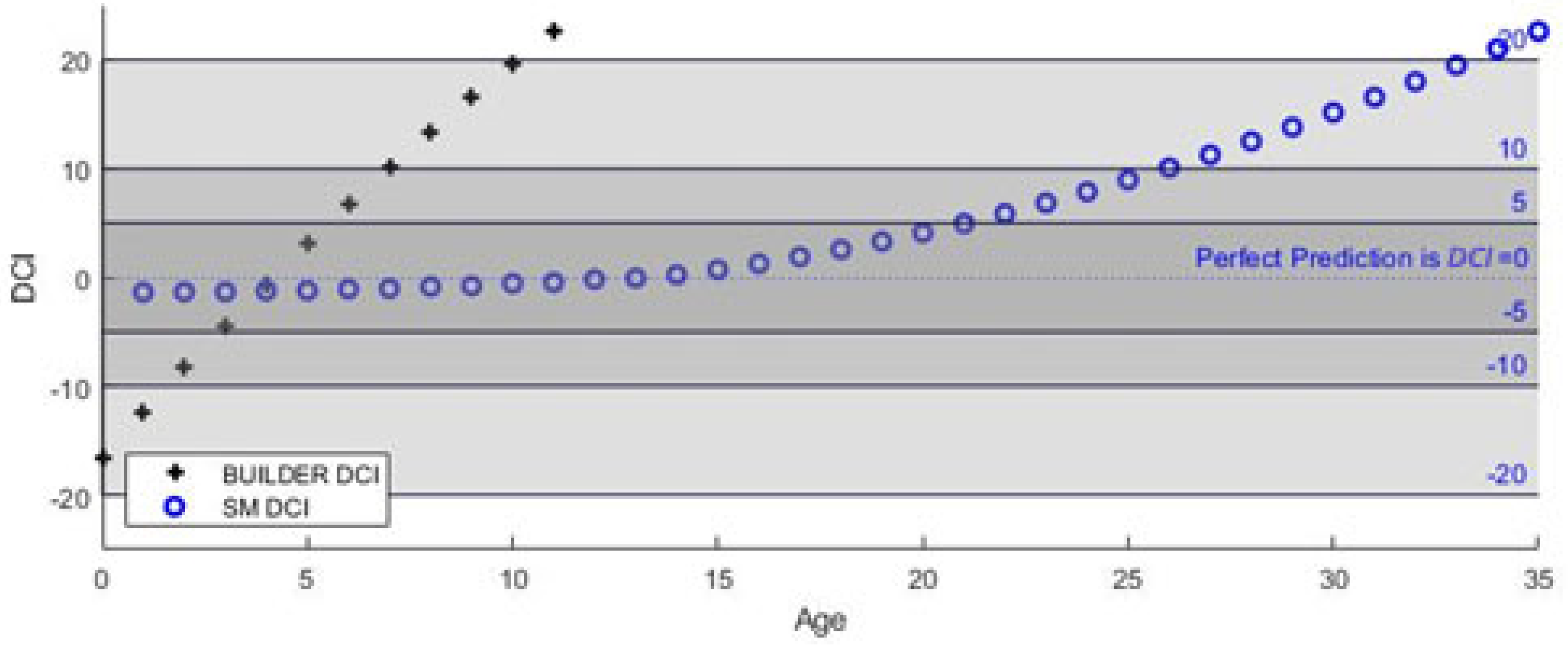
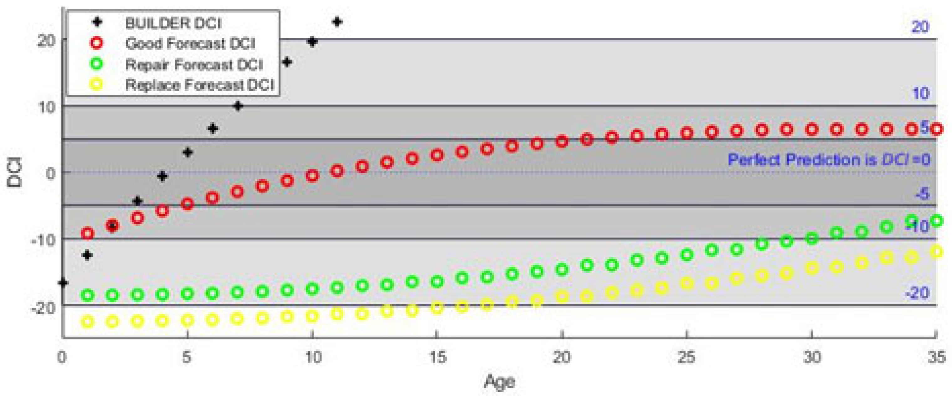
3.3. Condition-Intelligent Weighted-Slope Model (CI-W-SM)
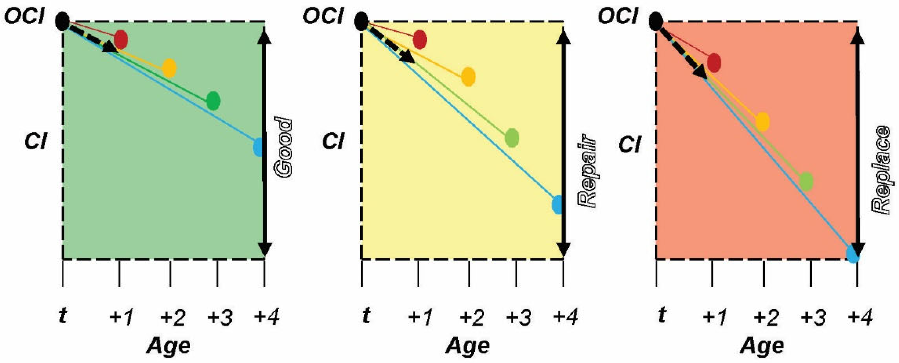
Methods: The third-generation model is the Condition-Intelligent Weighted-Slope Model (CI-W-SM), which adds condition thresholds to the W-SM and constrains asset selection to a condition performance category. This fine-tunes the model focus on assets with similar performance paths to make better predictions. This improvement allows the model to filter out assets performing better or worse than the asset in question, thus producing a more accurate degradation prediction as long as sufficient data are available. Within BUILDER SMS, performance categories of Good (100-81 Green), Repair (80-61 Amber), and Replace (60-0 Red) are used as general guides for managers. Here, BUILDER’s categories are used to subset the data before calculating an expected condition value. Decision makers should set these performance category thresholds to target their maintenance, repair, and replacement actions appropriately.
The CI-W-SM uses the same four-year proximity search of the data set to calculate a weighted average ECI (y) for an asset at age (x) to predict the next year’s condition, as shown in Equation (3).
where:
= the current condition of all asset at each timestep;
= the Expected Condition Index (ECI) produced by the model for the next year;
= the Observed Condition Index (OCI) of the asset in question at its last inspection;
= the number of years past the current inspection;
= the age of the asset(s);
= the weighted value assigned to each out-year;
= the average condition of Good category assets from each out-year;
= the average condition of Repair category assets from each out-year;
= the average condition of Replace category assets from each out-year.
As shown in
Figure 3 and
Figure 4, each of the bins has its own weighted-slope values for each age index. Finally, when predicting the target asset’s forecast value, the model first checks the last inspected OCI (
) before using the corresponding bin(s) to make a 1-year prediction. Additionally, when bootstrapping consecutive predictions past 1 year, the model adjusts the bins it uses for prediction to match the condition of the asset in question. Thus, when the CI-W-SM model makes a prediction that crosses the Good/Repair condition boundary of 81–80 CI, it stops using data in the “Good” bin and uses data from the “Repair” bin to run the next year’s prediction calculations.
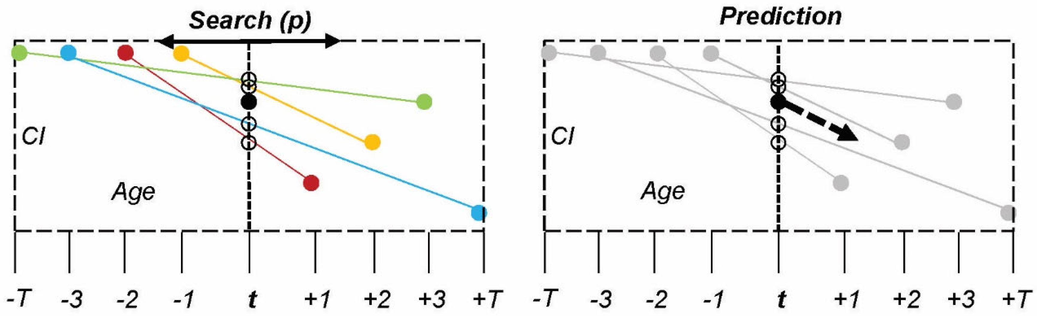
3.4. Nearest Neighbor Model (KNN)
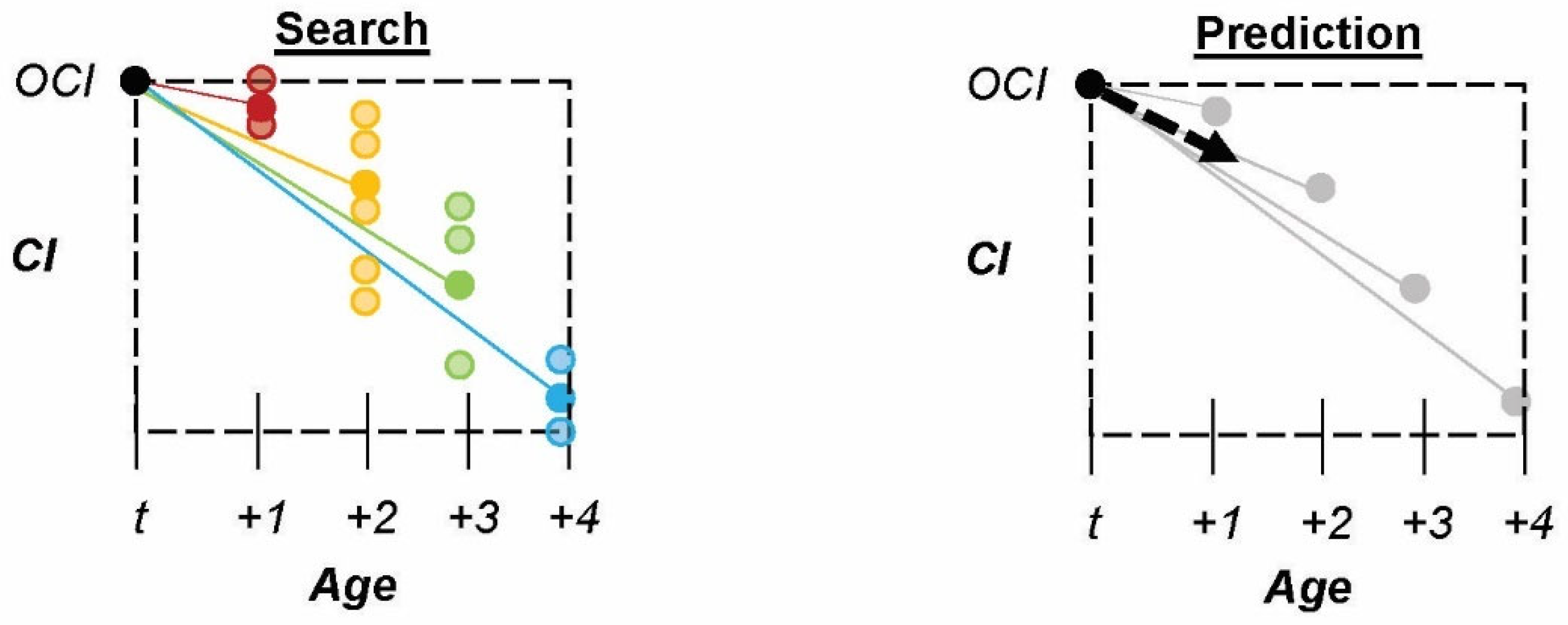
Methods: The fourth model uses a Nearest Neighbor (KNN) approach. This model differs from the others as it employs a radiating search space for neighboring assets starting at the target asset age (
), as shown in
Figure 5 and Equation (4). The search radiates outward by
year increments until it fills a minimum asset quota (
). Once
is satisfied, each asset’s condition slope is calculated; this slope represents the change in condition between the time at which the asset is retained, and its next assessment. The average of the
condition slopes is averaged to make a
prediction for the asset in question. The radiating search is unnecessary if the number of assets with condition assessments at age (
) is greater than or equal to
.
Furthermore, in this case, all assets with condition assessments are used to make a prediction so as not to limit the model’s data unnecessarily. This model assigns equal weight to all assets included in the search quota so that assets further away from the target asset in age are not penalized for their age difference. Note: This model’s outcomes vary based on the size set for minimum asset quota (
) because this directly changes the minimum size of the sample required to make predictions. A K value of 6 is used in this paper because it achieves satisfactory results when validated against known inspection data.
where:
= the Expected Condition Index (ECI) produced by the model for the next year;
= the first inspection condition (OCI) of each asset filling the quota ();
= the second inspection condition (OCI) of each asset filling the quota ();
= the number of years past the current inspection;
= the age of the asset in question;
= the number of years before ;
= the minimum number of assets in the quota;
= each asset in the quota.
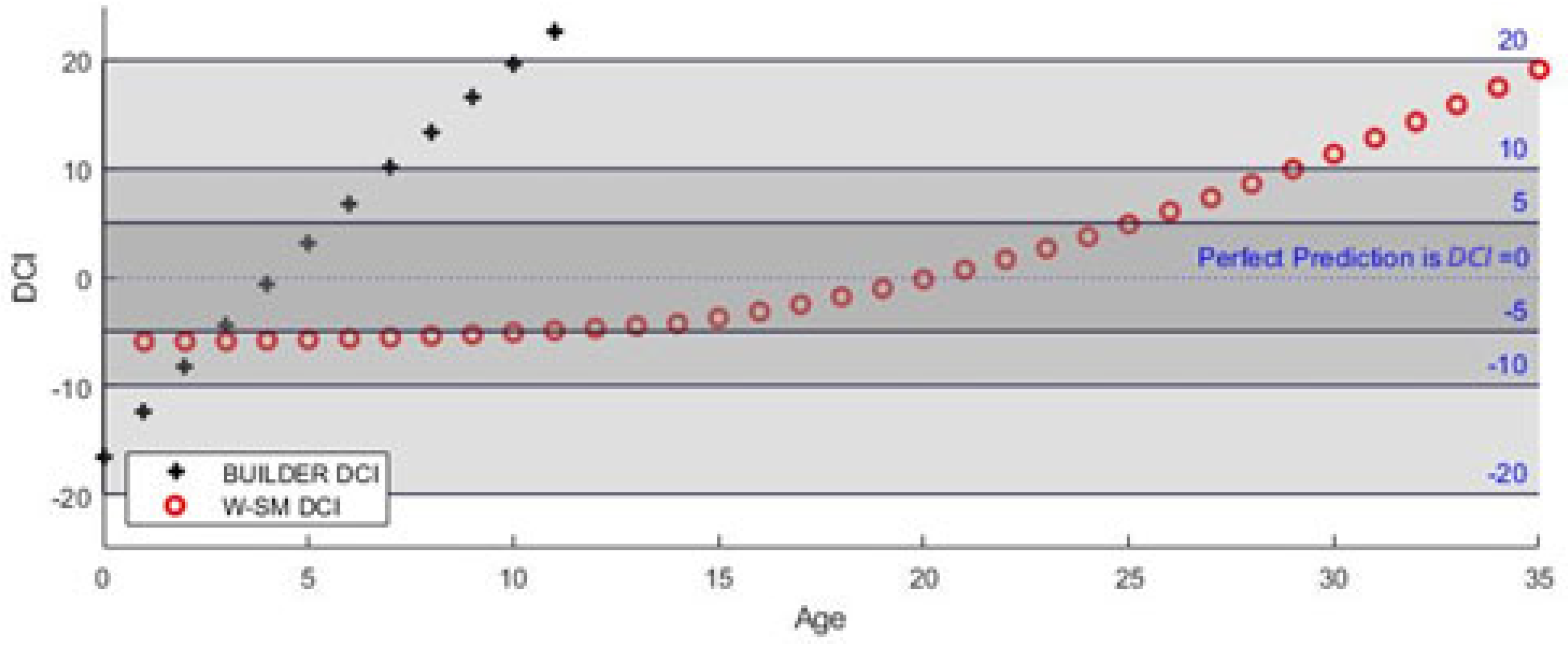
3.5. Model Validation
A framework was developed to compete the models using DCI as the validation metric. Simply put, DCI is the difference between the observed and forecast values. In this framework, a “win” is categorized by the model with the lowest DCI for an individual age within the service life so that the quantity of possible wins between the models is equal to the service life predicted by the W-SM. The individual results for the five researched roof system types were reported as well as a collective performance value for each model. The model value showed the overall win percentage for the model across all roof types.
4. Results
The four models are discussed individually in this section. Then, model validation is addressed collectively at the end of this section to show how the models compared to BUILDER SMS and to each other.
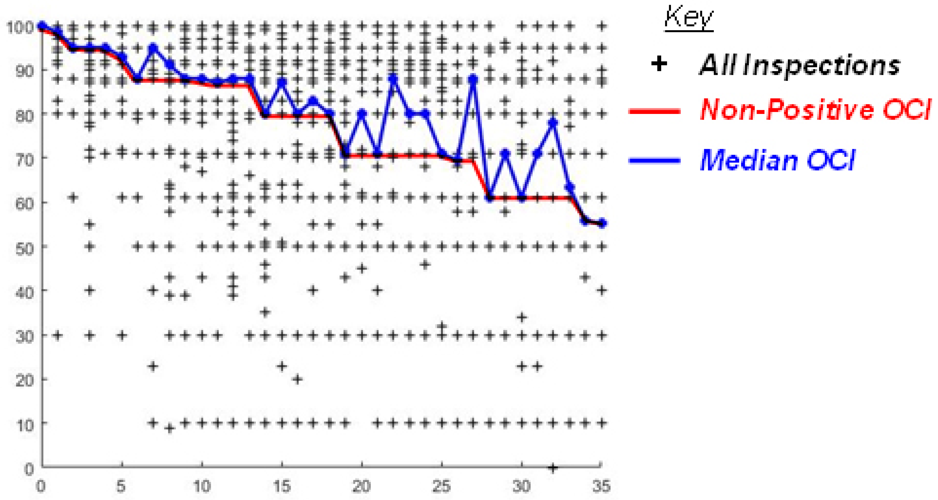
4.1. Slope Model (SM)
Results: While BUILDER data directly drive this modeling approach, the simplified single-year median produces ECI values that occasionally increase between predictions, see
Figure 6. This means that as the population data increases in age, it does not always decrease in condition, which causes large variations in the data distribution between years. Although an increase in average condition between asset ages is an accurate depiction of the data when taking single-year population medians, individual assets cannot behave this way because assets that increased between inspections were removed during data filtering. A non-positivity constraint was employed to combat the average condition increases between years. Unfortunately, after using the non-positivity constraint for this model, the degradation plateaued significantly due to the number of data points removed. As discussed in the data section, age was not highly correlated with condition. This model re-illustrates the limitations of directly correlating age and condition.
4.2. Weighted-Slope Model (W-SM)
Results: The four-year proximity-weighted averaging eliminates ECI value increases between predictions. The model only uses the data of assets that have inspections at the same age as the target asset and have an additional inspection at 1, 2, 3, or 4 years immediately after. In order to use the model values to predict future values of individual assets at different initial inspection conditions, the slope values are extracted from the weighted condition values, by taking the difference of expected values, and indexed by age. The plotted result of this model is shown in
Figure 7. Validation of this model is included at the end of this section.
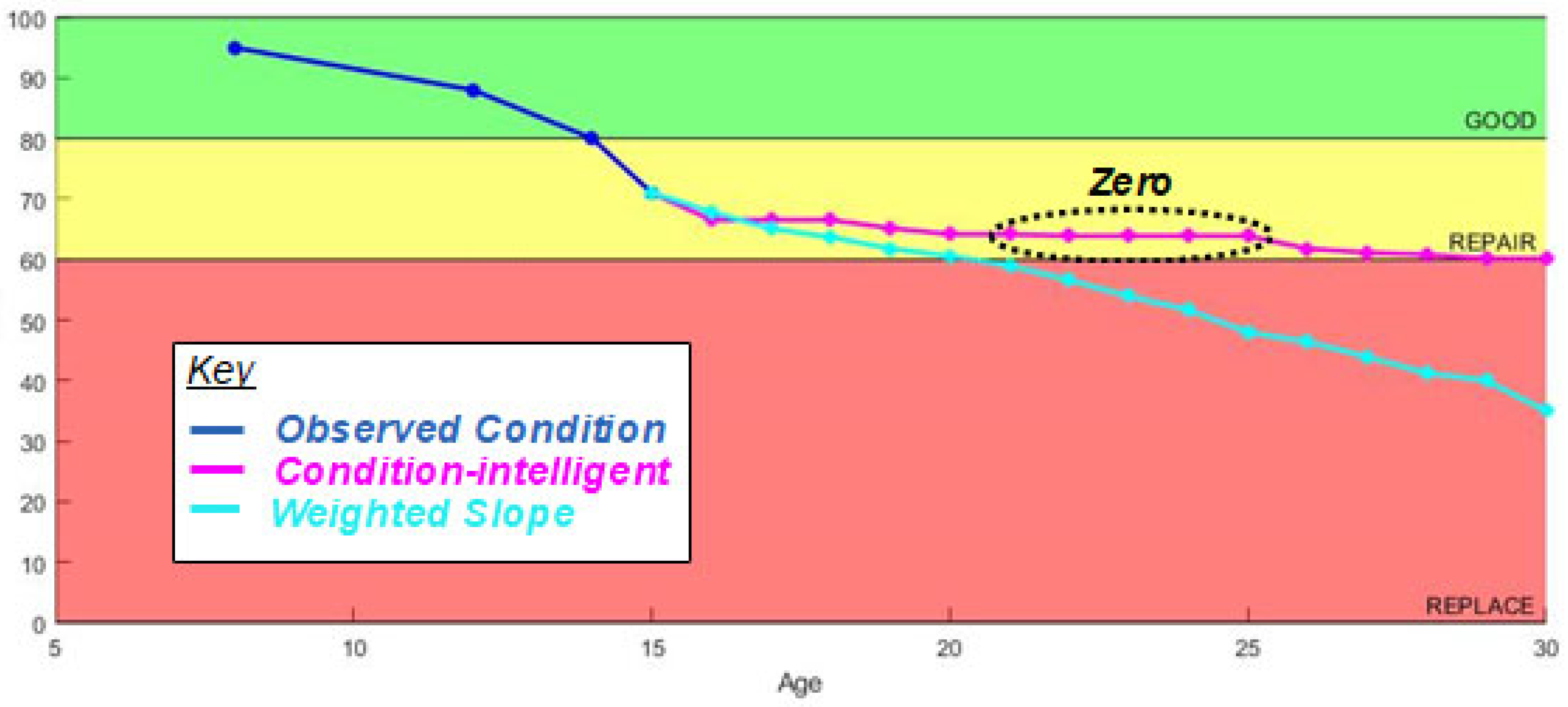
4.3. Condition-Intelligent Weighted-Slope Model (CI-W-SM)
Results: The four-year proximity-weighted averaging, such as the W-SM, eliminates ECI value increases between predictions but only uses the data of assets that pass through both the same age and condition category of the target asset. Because of this, the model becomes more optimistic, as it ignores assets outside the target asset’s condition bin (Green = Good, Amber = Repair, and Red = Replace). As discussed in the Data section, the categorical subdivision of the data reduces the number of assets in each prediction sample. While this approach should produce more realistic predictions, it does reduce the statistical significance of each prediction by reducing the sample size used to make the prediction. In years where there are not enough data to compute a prediction, this results in a prediction slope of zero, or no change from the previous year.
This model requires the highest data quantity, and data quantity must be sustained across the entire life cycle of the asset. In this specific data set, metal roofing (SSM) had the highest quantity of data and the longest life cycle, which produced the least no-change predictions (
Figure 8). Single-Ply membrane (SP) roofing had the second-lowest quantity of data and a significantly shorter life-cycle expectation, which resulted in the most no-change predictions (
Figure 9). These results suggest that data quantity is imperative for making service-life predictions using this model. Validation of this model is included at the end of this section.
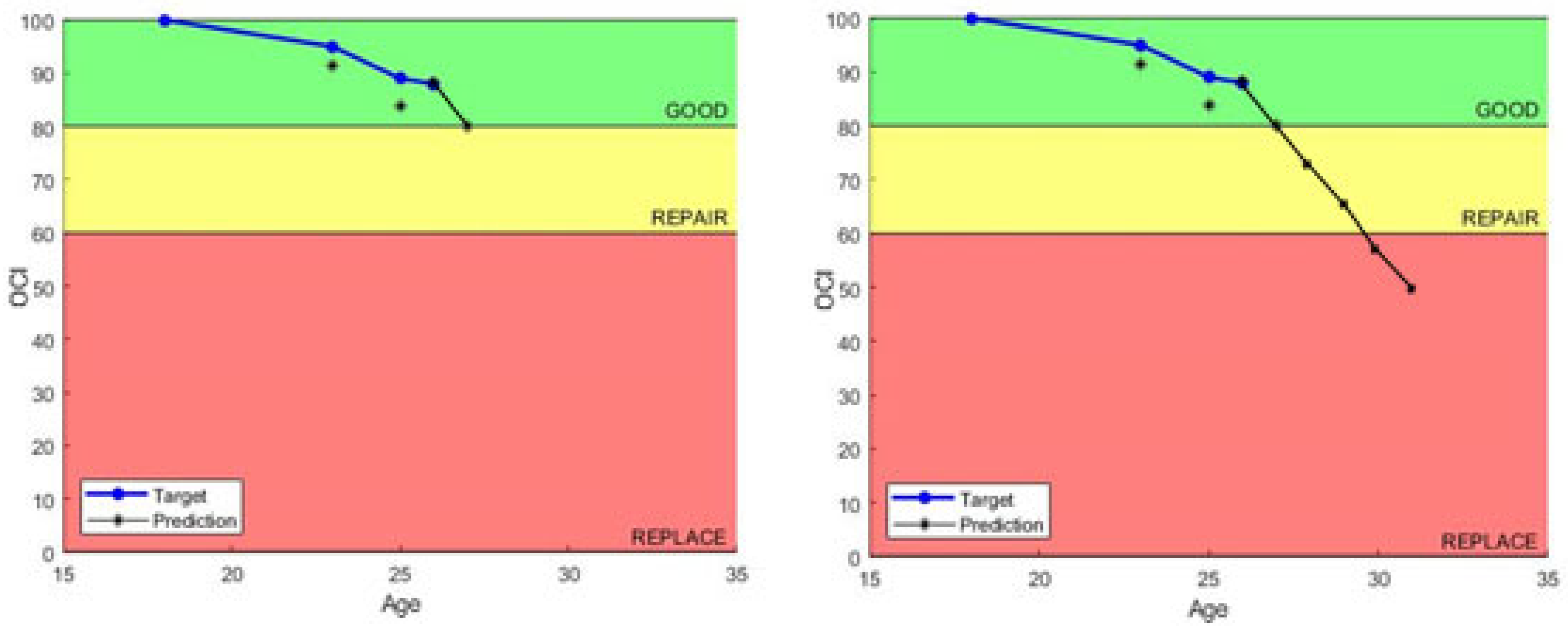
4.4. Nearest Neighbor Model (KNN)
Results: This model makes highly skillful 1-year lead predictions (
Figure 10). Notably, almost all 1-year prediction values produced by this model were within five CI points or less of the actual condition, which is very good. One example of the 1-year prediction accuracy is shown in
Figure 10, where the model predicted the value of the last recorded inspection with zero error (both points are on top of one another). In order to make long-term predictions of service life using this model, bootstrapping of the data is required. However, when bootstrapping is used, it quickly results in a compounded underprediction of the assets’ actual conditions. The most likely reason for this is that assets with catastrophic failures (or rapid degradation) are increasingly more likely as assets age. Since this model uses a varying number of years instead of a four-year average to make predictions, these rapidly failing assets have the potential to account for a significant weight in the average depending on the quota (
) size selected.
4.5. Model Validation
Three of the models ultimately competed against the predictions of BUILDER SMS. The Slope Model (SM), Weighted-Slope Model (W-SM), and the Condition-Intelligent Weighted-Slope Model (CI-W-SM) are reported because they all showed strong graphical performance when initially plotted. The prediction plots for each roof type produced results consistent with industry service-life. The results of these three models and BUILDER SMS predictions were compared to observed asset conditions to validate prediction skill. When comparing the SM results to the W-SM results, it became apparent that both had similar win percentages and similar shapes, but their y-intercepts varied. Ultimately, the rapid deterioration predictions that resulted from bootstrapping with the Nearest Neighbor (KNN) model made it unbeneficial for long-term service-life comparison.
The service life of each roof system type is determined by the number of years the W-SM outcomes remain in the Good/Repair bins. While manufacturers guarantee specific performance ranges for roofing products and systems, these data-driven results showed the actual average service-life ranges for each system installed at the 61 Air Force locations in this study. Initial validation of the W-SM showed that service-life predictions for the five roof types researched were similar to those of manufacturer specifications, suggesting validation of the W-SM as a service-life forecast method. The CI-W-SM was not used to determine service-life values for the roof types because all roof types contained years without data, which was a direct result of insufficient data quantity due to the additional subdivision of the data, as discussed in the results section.
The DCI validation metric discussed in the Methods section of this paper was used as the framework to compete the models. In this framework, a “win” was categorized by the model with the lowest DCI (
Figure 11,
Figure 12 and
Figure 13) for an individual age within the service-life range. The lower the DCI value, the better the model was at predicting observed conditions. The individual results for the five researched roof system types are reported in
Table 3, as well as a collective model performance value. Model values captured the overall win percentage for that model across all roof types. The W-SM outperformed the BUILDER SMS prediction an average of 92% of the time. The CI-W-SM beat the BUILDER SMS prediction an average of 69% of the time. For BUR, the W-SM resulted in an R
2 value of 0.38, while the CI-W-SM produced an R
2 value of 0.39, and the BUILDER SMS R
2 value was 0.06. Additionally, the root mean square error (RMSE) values for the W-SM, CI-W-SM, and BUILDER SMS were 32.81, 39.26, and 49.83, respectively. Individual results for the five roof sub-types are shown in
Table 3.
5. Discussion
Stepwise data-driven modeling techniques can be used to calibrate degradation forecasts based on observed conditions and improve the correlation between asset age and condition. As asset data continue to grow in quantity, the results of these models are likely to change. A discussion of the models and their response to increased inspection data quantity over time is detailed below to explain the models in more depth, as summarized in the model wrap-up shown in
Table 4.
Decision Making: The four models discussed in this research demonstrate that while some methodologies are beneficial for short-term predictions, those same models may not be skilled at predicting an asset’s service life. For this reason, the models created were categorized into short-term or long-term categories based on their unique skills. Short-term models are those that make skilled near-future predictions, such as the KNN model discussed in this paper. The KNN model makes strong 1-year forecasts, but it lacks the skill to make predictions further into the future. This type of model helps analyze assets close to decision points, deciding whether an asset will likely need a repair or replacement project in the coming year, or whether it will remain relatively stable. Long-term models are characterized by their skill in forecasting the service-life degradation of assets, which may be years or decades away. While current service-life models traditionally blanket-apply singular population averages to every asset uniformly, the other three models discussed in this paper show that a stepwise, data-driven approach is more accurate than continuous statistical functions because stepwise methods look at rates of degradation instead of targeting a single service-life age. This makes the SM, W-SM, and CI-W-SM great planning tools for enterprise-wide asset management efforts such as those frequently drawn from BUILDER SMS. As asset management progresses, aligning model types to decision-maker priorities should be as much a focus of the industry as building accurate degradation forecast models.
Ensembles: In reality, decision makers typically exist at all levels of agencies, and their priorities vary based on their level of authority. For example, an enterprise-level decision maker may set corporate budgets for facilities maintenance and repair, while a program manager may hold the responsibility for selecting individual projects and assets to utilize funds as they become available. These differences make it difficult to justify the use of a single forecast model. This is why understanding the goal of decision makers should inform the types of models used to analyze data. While it may be more complex, combining each model’s benefits into an ensemble may be more informative and skillful for making holistic asset predictions. This type of approach may be able to inform and satisfy both types of decision makers simultaneously, and the effort of combining stepwise models becomes quite easy to automate through the use of index values as is done in the CI-W-SM for assets when they transition from one condition bin to another. The versatility of stepwise modeling to include the aggregation of multiple models via indexing is another potential advantage of the proposed framework.
6. Conclusions
Although asset management methodologies have been in place for decades, the methodologies used for employing asset management data to predict future conditions are still evolving as new data become available. Existing prediction models produce broad life-cycle expectations from population averages instead of data-driven, asset-specific condition expectations. This research employed roofing data from 61 unique US Air Force locations to show that stepwise methodologies can be superior to the industry-leading continuous methodologies employed by BUILDER SMS in service-life prediction accuracy and decision-making versatility as ensembles. Notably, the data used to train the models created were also used to test them; however, the stepwise fashion employed by the models does exclude future conditions of target assets when making predictions. This means that bias in these models should be minimal if at all present. These methodologies should be employed using an alternate data set to validate and compare the results. As discussed in the Data and Case Study section of the paper, there is much room for improvement in the area of data retention, and for this reason it is suggested that modifications to the BUILDER SMS database or a more complex pre-filtering methodology be considered. This improvement would allow any repaired or replaced assets to be retained in the calculations as new entries instead of a continuation of the repaired/replaced asset. Improvements of this kind would increase overall data quantity, sample sizes used to make predictions, and model forecast power without introducing confounding data.
Future research is suggested to refine and validate the findings of this case study. Roofing systems were analyzed in this research due to their variety of service-life durations. While the data used for this research are specific to roofing assets, using the same methodologies to analyze all BUILDER SMS assets is the broader intent. For this reason, it is recommended that other asset types such as exterior wall systems, mechanical equipment, structural elements, and other facility component types be analyzed using the proposed stepwise approach to study the assumptions and any necessary adjustments for other asset types. While results are anticipated to be similar, the K-value in the KNN model and the number of years (n) used for proximity weighting of the W-SM and the CI-W-SM are relatively new, and further research and statistical analysis of these variables may offer opportunities for optimization as future improvement opportunities. The concept of the Delta Condition Index (DCI) provides a consistent metric for comparing future model results in a uniform metric, and additional research into statistically fitting the DCI of each asset subtype as a continuous function may provide breakthroughs into rapid improvement to the current BUILDER SMS degradation formula.
Nevertheless, the asset management industry must move away from just focusing on when a component will fail and consider the strategic points throughout a component’s life when targeted maintenance or repair may be beneficial. Moving towards more intelligent stepwise models is one way to increase the understanding of an asset’s middle-life. This transition will also enable decision makers at operational levels to make stronger predictions of short-term asset performance, thus capitalizing on right-time planning for asset-specific repair and replacement projects. The four new models discussed in this research can be used as short-term, long-term, or ensemble forecast tools that elevate the prediction power of asset managers of all levels, even as data quantity expands. While individual models may be best suited for some decision makers, ensembles that employ the indexing power of the stepwise methodologies developed in this research are likely to provide the most comprehensive asset overview yet published.


