Abstract
To address the problem of sensor faults and measurement noise being misinterpreted as structural damage in structural health monitoring (SHM), this paper proposes a new framework for distinguishing sensor faults and structural damage based on stacked gated recurrent neural networks (S-GRU NN) that considers measurement noise. In this framework, the sensor signal reconstruction model was constructed by learning and training the S-GRU NN. The sensor fault threshold was determined based on a statistical analysis of the response reconstruction error between the true and reconstruction values. The sensor fault and structural damage are then distinguished by the fact that the sensor fault is independent and the structural damage is global. The framework is compared with other isolation frameworks based on traditional deep learning models through numerical simulations of a three-span continuous beam and laboratory steel frame experiments. The results show that the S-GRU NN has better reconstruction effect and isolation performance of sensor faults and structural damage in noisy environment.
1. Introduction
Structural health monitoring systems have been popularized and applied to many large civil structures. It is of great relevance to the safety and stability of large structures, but many challenges remain, especially abnormal changes owing to sensor failures and measurement noise. As the front-end equipment in the monitoring system, sensors are the main means of obtaining various environmental and structural response information. The sensor performance directly affects subsequent structural damage identification and safety assessments [1,2]. The real operational state of the system can be correctly reflected only when the data measured by the sensor are stable and reliable. Conversely, the predictive results of structural health-monitoring systems may be problematic. However, in practical settings, degradation of the sensor performance is inevitable because of structural material degradation and complex environmental influences [3,4]. In such cases, the measured structural response and vibration characteristics change, and may be misinterpreted as structural damage [5]. Therefore, the SHM system requires an isolation method for sensor failure and structural damage that is not sensitive to noise.
The methods of sensor fault detection and identification include model- and data-driven methods [6]. Among them, the data-driven method has become the mainstream method of sensor fault detection because it avoids the limitation that complex structures are difficult to accurately model [7,8]. Dunia et al. [9] used the sensor reconstruction information to verify the original measurement results of the model. By analyzing the residual reconstruction of different variables, the sensor effectiveness index was determined, which distinguishes abnormal operating conditions from single sensor failure. Tharrault et al. [10] proposed a fast two-step algorithm for sensor-fault isolation. First, a robust model for outliers was established using the scale-m estimator, and then the resulting residual was generated based on the reconstruction principle. This method has been effectively applied in outlier detection for multi-fault scenarios. Sharifi and Langari [11] presented a sensor fault-monitoring and separation method for nonlinear smart structures. This method analyzes the detectability and isolation of each sensor’s faults and uses the Bayesian probability analysis of the residual to determine the error probability of each sensor. However, the above methods do not consider the influence of environmental changes on the sensor measurement results [12].
Lee et al. [13] proposed a new framework for identifying sensor faults of an inherently dynamic system. They first reconstructed the noise in the dynamic process, obtained the optimized reconstruction measurement results based on the optimization results of the time-delay data, and proposed a fault isolation index. Huang et al. [14] established a statistical hypothesis testing model for the sensor fault detection process and isolated fault sensors using the missing variables method. However, none of the above methods solves the problem of distinguishing signals from sensor faults and local structural damage in a dynamic noise environment.
In recent years, deep learning has achieved good performance in the field of SHM. It directly extracts valuable information from data via superposition of multiple nonlinear processing layers in a layered architecture; thus, it is superior to the traditional intelligent method [15]. Fan et al. [16] reconstructed sensor signals from structural failures using densely connected convolutionalneural networks networks (CNN). Zhuang, Y. et al. [17] proposed a data-driven structural fault detection method based on convolutional neural networks. Rosafalco, L. et al. [18] proposed a damage detection method based on a full-convolution neural network that detects structural damage by analyzing the original vibration measurement data of the structure. In contrast to CNNs, recurrent neural networks (RNNs), especially long short-term memory (LSTM) and gate recurrent units (GRU), are specially designed to learn the regression problems of sequential, time-varying, and linear/nonlinear modes [19]. Because the nonlinear response of structures is affected by both current and past time states, the RNN with the memory element performs better in the response prediction of nonlinear structures [20]. Zhang et al. [21] proposed an improved deep LSTM neural network to predict the seismic response of nonlinear structures. Liu et al. [19] proposed a sensor fault detection method based on LSTM. Compared to LSTM, GRU reduces the training time without affecting the model performance [22]. Thus, GRU has great potential in response modeling and prediction for nonlinear structures. However, deep learning-based anomaly detection methods require a large amount of structure monitoring data for model training and learning. The monitoring data during the operation of the structure is inevitably affected by environmental changes. Changes in the environment usually result in changes in the system. The influence of this change is often the same as that of the damage to be detected, which affects the reliability of structural damage identification. Whilst existing methods show strength under some noise, they become weak when the data set contains a large number of outliers. This is because most models are based on the mean square error (MSE) criterion, which is sensitive to outliers. Studies have shown that introducing a regular term in the loss function can reduce the weight of a large number of simple samples in the training and allow the model to focus more on difficult, misclassified samples, thus improving the robustness of the model [23].
In this study, a new framework is proposed to analyze the isolation performance of sensor faults and structural damage, considering the influence of measurement noise. Based on the deep neural network theory, a stacked GRU structure response reconstruction model was proposed, and the anti-noise performance of the model was improved by introducing a regular term. The error between the measured and reconstruction values of the sensor was used to detect sensor failure and structural damage. This framework is suitable for cases where a single sensor has failed over a period of time. To investigate the accuracy and robustness of the proposed framework, numerical simulations were performed on a concrete three-span continuous beam, taking into consideration the influence of environmental noise. An experimental study on the frame structure model was conducted to verify the performance of the proposed framework. Compared to traditional artificial neural network-based frameworks, the isolation framework proposed in this paper has higher accuracy in noisy environments.
2. Theoretical Explanation of the S-GRU NN
RNNs are neural networks specifically for time series regression problems and have great potential for structural response modeling [21]. Among them, GRU and LSTM effectively avoid the problem of long-time sequence gradient explosion by gate structure. GRU and LSTM have similar accuracy, but GRU is more efficient to train [22]. Therefore, the GRU-based neural network model is used for structural response reconstruction. Meanwhile, the acceleration response of the structure is a time series, and the structural response is affected by factors such as temperature and air humidity. Due to the influence of various factors, adding fully connected (FC) layers can improve the model reconstruction performance [24].
The S-GRU NN model uses the loading signal of the structure or the measured signal of a certain sensor as input data, and the measured signals of other position sensors are used as output data. This model is composed of a stacked GRU layer and multiple fully connected layers. The function of the stacked GRU layer is to capture long-term data dependencies and model time-series data. To improve the model’s reconstruction performance and generate the appropriate number of output features, fully connected layers are utilized to connect the stacked GRU layer to the target and target-output layer. This section describes the proposed network model in detail.
2.1. Gate Recurrent Unit
The GRU is a special type of RNN with a weighted connection, memory, and feedback function. GRU overcomes the vanishing gradient problem of traditional RNNs, therefore it can realize the learning of relatively long time series [22,25]. Figure 1 shows the basic architecture of the GRU, which consists of an update gate zt and a reset gate rt at time t. The z is used to determine which part of the current hidden unit should be updated by the candidate hidden state , while the r is used to determine which part of the previous hidden state h is ignored. During the training of the neural network model, the gradient is inverted to update the parameters of the GRU with the optimization objective of minimizing the loss function.

Figure 1.
GRU structure diagram.
2.2. Stacked GRU Neural Network
The acceleration of the structure’s current time node is affected by the acceleration of the previous period and is affected by environmental factors such as temperature and humidity [26]. To improve the reconstruction performance and robustness of the model in different environments, this paper proposes a stacked sequence-to-sequence GRU NN with FC layers.
The input X and output Y acceleration sequences of a traditional GRU are denoted as
where j and k are the characteristic numbers of the input and output data, respectively.
The principle of the stacked gate recurrent unit network model is illustrated in Figure 2. This format makes use of stacked inputs with a set number of time steps (such as d steps), that is, , to reconstruct the output y. To explain the concept of S-GRU NN more specifically, we take an example where the input and output data of the model have only one dimension (i.e., j = k =1).
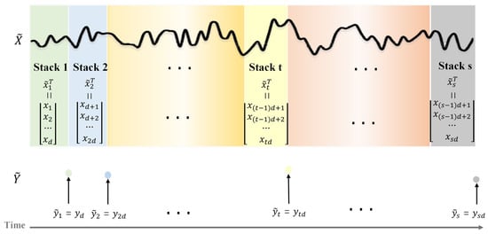
Figure 2.
Schematic diagram of stacked GRU. Where, t = 1, 2, … s, sd = n.
The input acceleration sequence X = and output acceleration sequence of the structure are divided into multiple stacks, and the form of the new input and output acceleration sequences, and , respectively, are as follows:
where, s is the number of stacks.
Each stack is then regarded as a timestamp, and the total number of timestamps is s. It is worth noting that each new timestamp input comprises the data of time nodes in the original sequence X. The input sequence and output sequence at the t-th timestamp can be expressed by Equations (5) and (6):
where d is the length of each stack.
To further enhance the performance of the network model and construct the desired output features, we added FC layers to the stacked GRU layer. The FC layers were fully connected to all activation points of the stacked GRU layer. An FC layer adds bias vector b to the input after multiplying it by a weight matrix w. This model is called the S-GRU NN, and its architecture is shown in Figure 3.
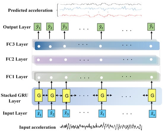
Figure 3.
S-GRU NN architecture.
The activation functions of the stacked GRU layer, FC1 layer, and FC2 layer are the Relu function. Relu functions have the characteristics of simple calculation, more efficient and fast, and it is widely used in the prediction and classification of time series [18,21]. In order to ensure that the model can output the reconstructed response that meets the actual requirements, the activation function of FC3 layer is linear activation function. The input and output sequences of the S-GRU NN structure must be a three-dimensional dataset. The first dimension is the number of samples m, second dimension is the time series l, and last dimension is the feature number q. In this study, the input acceleration of the structure or the acceleration measurement value of the reference sensor were used as the input data. The measured signal of the sensor to be detected was the output data. The input data can be the acceleration sequence of a single node or a combination of acceleration measurements from different nodes. The number of input data characteristics is equal to the number of structural reference nodes. Likewise, the number of output data features equals the number of sensors that need to be detected. It is worth noting that the traditional GRU network model pays more attention to the input signal of the current time node in the reconstruction process of the current times node, while in practical engineering, the collected monitoring signal inevitably has noise, and if the input signal of the current time node is heavily contaminated by noise, it will affect the reconstruction result of this times node. The unique stacked format allows the S-GRU NN to focus more on the state of the timestamp in which it is located during the reconstruction of the current time node signal, which avoids the problem of increasing reconstruction error due to the input signal of a single time node being heavily contaminated.
2.3. Dropout
To prevent overfitting of the model, dropout technology is introduced into the network structure. The aim of dropout is to reduce the parameters of the model involved in the calculation during each training by randomly disconnecting the neural network. However, in the test stage, dropout restores all connections to obtain the best performance [27].
2.4. Loss Function
During the training process, S-GRU NN was used to reconstruct the response signal of the sensor to be detected, and the goal of the model training was to greatly reduce the difference between the reconstructed and measured responses. Therefore, we estimated the reconstruction performance of S-GRU NN using the root-mean-square error (RMSE) between the measured and reconstructed signals. To enhance the generalization ability of the S-GRU NN model, we added a parameter sparsity penalty to the loss function. The new optimization objective of S-GRU NN is
where, is the original loss function, y is the measured actual acceleration, is the reconstructed acceleration, is the L regular term, w is the weight vector, is the regular-term coefficient, and = 0.1 in this study.
The new optimization objective forces the loss function reduce RMSE while reducing the weight of unimportant features as much as possible, and the weight relationship between them is adjusted by . The fundamental idea is to reduce the probability of noise in the model-fitting training set by limiting the size of the weights, thereby enhancing the robustness of the model [28].
3. Isolation Strategies for Sensor Failure and Structural Damage
3.1. Sensor Failure Model
Owing to the limitations of environmental influences, external load influences, and performance degradation of the sensor itself, sensors placed in civil engineering structures fail over time. Because the sensor failure model summarized in multiple studies is relatively mature, it is similar to the failure of the sensor installed in the actual structure [11,29,30]. In this section, four common sensor failure models are constructed to better simulate sensor failures. They have proved to be similar to actual sensor fault signals and were widely used in sensor fault research [5,29,30,31].
3.1.1. Bias
Bias refers to the measured structural response resulting in a constant offset, which typically occurs when the sensor base becomes loose. The bias model is expressed as follows:
where is the measured value of the sensor, is the actual structural response, A is a constant, and is white Gaussian noise.
3.1.2. Gain
Gain is a sensor performance degradation model that increases exponentially and is usually caused by voltage instability. The model can be expressed as follows:
where G is the unknown gain coefficient that may change several times during the actual measurement.
3.1.3. Constant Fault
A constant fault is a type of complete sensor fault. The signal is a constant with noise fluctuation, and its model is as follows:
3.1.4. Background Noise
Background noise is another type of complete sensor failure, and the signal only shows the noise model, that is,
The above models have been proved to be effective for sensor fault detection research [14,24]. In this study, parameter A is equal to the average value of the normal signal. The gain coefficient G was 1.6. is the Gaussian white noise whose amplitude is scaled such that its maximum value is the mean of the normal signal. The signals of the four sensor-fault models are shown in Figure 4.
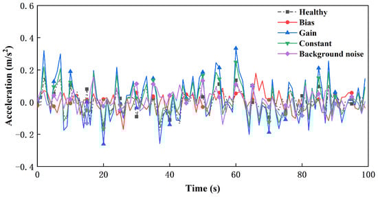
Figure 4.
Healthy signal and signals with sensor fault.
3.2. Fault Threshold
As a statistical method that describes the discrete distribution of data that is relatively stable and less affected by outliers, the box-plot plays a major role in the field of data mining and outlier detection [32,33]. The box-plot usually consists of five value points: the lower edge, 25% quantile (Q1), median, 75% quantile (Q3), and upper edge. The distance between Q1 and Q3 is called the interquartile range (IQR). The structure of the box-plot is shown in Figure 5.
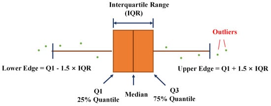
Figure 5.
Generic architecture of box-plot.
During anomaly detection, sufficient data on the structure in its normal operation state are first obtained, and various learning parameters in the network are initialized. The acquired data are then sent to the S-GRU NN model for data fusion and training. The measurement signal of the sensor is reconstructed via iterative update learning. The residuals of the reconstructed and measured values can be obtained as
Then, the average reconstruction errors (ARE) of sensor signals at each timestamp in all training data were calculated. The ARE can be expressed as
where m is the number of training samples, that is, the first dimension of the input data in Section 2.2.
A box diagram of each sensor’s average reconstruction error was drawn, and their upper edge was calculated. To analyze the objectivity and robustness of the threshold, we took the maximum upper-edge value of the average reconstruction error for all sensors as the threshold. The threshold can be obtained as
where q is the number of sensors to be detected, that is, the third dimension of output data in Section 2.2.
3.3. Isolation Strategy
An abnormal structural response includes both sensor failure and structural damage. The abnormal structural response caused by a sensor failure is an independent event, whereas the structural response abnormality caused by structural damage is a regional series of events. In other words, for a global sensor system (such as an acceleration sensor), sensor performance failure can only cause abnormalities in the response collected by the faulty sensor. However, when the sensor is damaged locally, multiple sensors near the damaged location will also pick up abnormal signals. Based on the above discussion, the process of isolating sensor failure from structural damage is illustrated in Figure 6.
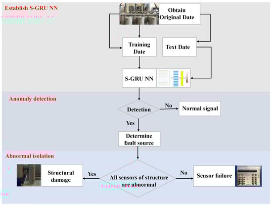
Figure 6.
Isolation process.
The specific operation steps are as follows:
- (1)
- Sensor data for structural health is obtained under different environmental or operating conditions.
- (2)
- Data preprocessing: the loading signal or reference sensor signal of the structure is taken as input data, and the measured signal of the sensor to be detected is taken as output data. Training and validation datasets are then divided.
- (3)
- A S-GRU NN is constructed, and training and reconstruction are conducted for the sensor signals.
- (4)
- The threshold of the training sample’s reconstruction error is calculated using Equation (14).
- (5)
- A new set of signals is passed into the network and the reconstruction error of all sensors is calculated.
- (6)
- The box-plot of each sensor signal reconstruction error is drawn, and the edge value of the box-plot is compared with the threshold .
- (7)
- If the upper edge of the box plot exceeds the threshold , it indicates structural damage or sensor failure.
- (8)
- If sensors in a certain area of the structure are detected to be abnormal, this area has structural damage. Otherwise, one of the sensors is faulty.
4. Numerical Studies
Referring to the literature [34,35], we used a three-span continuous beam model as shown in Figure 7 to generate training and validation data and to evaluate the correctness of the S-GRU NN for signal reconstruction. The beam element in ABAQUS was used for the structural analysis. The length of the model structure was 40 m, and its cross-sectional area was 0.25 × 0.6 m. The model is divided into 200 equal cells, each with a length of 0.2 m. The mass density of the material is 2400 kg/m3, elastic modulus E is 30 GPa, Poisson’s ratio is 0.3, and damping type was set to Rayleigh damping. Referring to the method in the literature [24], Gaussian white noise with a maximum amplitude of 0.4 m/s2 was used as excitation and applied to each support at the same time. The dynamic reaction of the structure was captured by ten acceleration sensors (S1–S10) positioned on the beam. The sampling frequency was 100 Hz and 300 data samples with a duration of 10 s were obtained. In general, a response time series of 10 s is adequate for a network to learn the characteristics of the data [36]. As the time series increases, the model’s generalization ability becomes more powerful, but increases the requirements and computation of the CPU. Referring to the method in the literature [34], the elastic moduli of the ten beam elements in the middle of the central span were reduced by 5, 15, and 25%, respectively, to simulate three different degrees of damage, as shown in Figure 7.
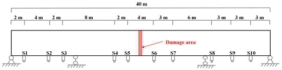
Figure 7.
Three-span continuous beam model.
4.1. Data Preparation
Each sample was composed of the excitation acceleration at the support as the input and the measured value of each acceleration sensor as the output. Referring to literature [16,21], the entire dataset was split into three subsets: 160 samples in the training dataset, 40 samples in the validation dataset, and 100 samples in the prediction dataset, which is assumed to be an unknown dataset for testing the performance of the training model. All subsets were formatted according to the S-GRU NN standards described above. Because S-GRU NN uses a stack size of d = 5, the time step is 1000 data points in 10 s, and the number of sensors to be reconstructed is 10, the input and output sizes of the training dataset are [160, 200, and 5] and [160, 200, and 10], respectively, and the input and output sizes of the validation dataset are [40, 200, and 5] and [40, 200, and 10], respectively. In addition to the input and output layers, the parameters of the stacked GRU layer, FC1 layer, FC2 layer and dropout layers need to be set. We have optimized the parameters using the vertical comparison method [37], i.e., when analyzing the effect of one of the parameters on the prediction results, the rest of the parameters are fixed and the optimal range is derived from literature [21,38,39,40]. The optimized network parameters were set as follows: q (stacked GRU) = 100, q (FC1) = q (FC2) = 128, and the dropout layers were added to the stacked GRU, FC1 and FC2 layers at a rate of 0.3.
The input and output of the training dataset were sent to the S-GRU NN model for training, with a batch size of 20. A gloot unified initializer [41] was used to randomize the weights of all stacked GRU and FC layers, and the deviation was set to zero. To accelerate the convergence speed of the training model, we choose the adaptive momentum estimate as the optimizer, with a learning rate of 0.001 and an attenuation rate of 0.0001. There were 2000 epochs in the training phase. To improve training performance, the minmaxscaler in the scikitlearn toolbox [42] scaled all data to [−1,1]. In addition, training data were shuffled before each calendar element to reduce model variance [43].
The effectiveness of the optimal combination S-GRU NN after training was verified using the validation data. The GRU, LSTM [21] and CNN [17] were employed for comparison with our method. These three algorithms adopt the traditional artificial neural networks data format shown in Equations (1) and (2), and used the same batch and training phases as S-GRU NN.
To simulate the measurement noise, the acquired structural acceleration signal was polluted by applying Gaussian white noise with a signal-to-noise ratio (SNR) of 40 and 60, respectively. The chosen SNR represents the self-noise of the accelerometers commonly used for civil structure monitoring [18,44]. The noise-containing dataset was divided using the above method, and then the divided training dataset was sent to each of the four network models for training, so as to investigate the reconstruction performance of S-GRU NN in noisy environments.
In order to measure the reconstruction performance of different algorithms, the relative error of the reconstructed response was quantified using the method in literature [16], and the quantified relative error was denoted as
where A is the reconstructed acceleration and A is the true acceleration.
4.2. Reconstruction Results
Predicted data were fed to three sets of models trained on data at three noise levels to evaluate the accuracy of reconstructed responses under new environmental conditions. Since the focus of this paper is on the isolation of structural damage and sensor faults in a noisy environment, the accuracy of signal reconstruction in a noisy environment has an important impact on the performance of the isolation framework. Figure 8 and Figure 9 show examples of the reconstructed response compared to the true response at 60 SNR and 40 SNR levels of noise contamination, respectively. Figure 10 shows the relative errors of signal reconstruction using the above four network models in the noise-free and two noise-level environments.
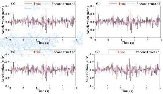
Figure 8.
True and reconstructed response signals of S9 in the noisy environment with 60 SNR. (a) S-GRU NN; (b) GRU; (c) LSTM; (d) CNN.
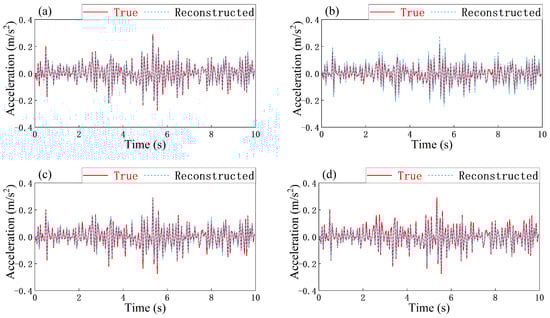
Figure 9.
True and reconstructed response signals of S9 in the noisy environment with 40 SNR. (a) S-GRU NN; (b) GRU; (c) LSTM; (d) CNN.
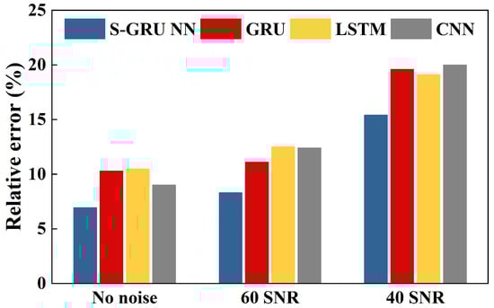
Figure 10.
Relative error of the reconstructed signal.
It can be found in Figure 8 that all four models can effectively reconstruct the signal of the failed sensor under the condition of slight noise pollution. However, the noise causes the local characteristics of the signal to change, both the peaks and troughs of the reconstructed signal are different from the true signal. It can be found from Figure 10 that the reconstructed signal obtained by using S-GRU NN has smaller error. This is because the unique stacked structure of S-GRU NN allows the model to take more into account the input acceleration of the current time node and the four previous time nodes in the output of the acceleration of the current time node, avoiding the problem that the signal of the current time node is heavily contaminated by noise that makes it difficult for the model to capture the local characteristics of the signal. The loss function with regular constraints also reduces the probability of noise in the training set by limiting the size of the weights, which further improves the generalization ability of the model.
It can be found in Figure 9 that the accuracy of the reconstructed signals obtained using all four algorithms decreases when the measured signals are contaminated with high levels of noise; however, the S-GRU NN retains more detailed characteristics. The reconstructed signal obtained by using GRU and LSTM is similar to the true signal in the whole, however, as the input of the neural network, the state of the current time node has a greater impact on the output of the current time node. When the input of the current time node is heavily contaminated by noise, the model has difficulty in learning the local characteristics of the signal, resulting in the output signal losing more details. The network unit of the CNN uses pixel-to-pixel learning, and the input signal of the current time node still has a large influence on its output signal, so it is also difficult to accurately learn the local characteristics of the signal in a high-level noise environment. Unlike the above three algorithms, S-GRU NN is more concerned with the input signal of the timestamp where the current input node is located. Even if there is a lot of noise in the training data, the model is still able to learn the structural signal characteristics for a long time with a global view, while better capturing the local characteristics of the signal with a local view. Thus, the reconstructed signals obtained by S-GRU NN retain more local features.
The comparison of the reconstruction errors of the four algorithms shown in Figure 10 also reveals that S-GRU NN is able to learn the local features of the structured signal better, especially in the presence of measurement noise in the training data in the case of better reconstruction performance.
4.3. Sensor Failure and Structural Damage Isolation Framework Analysis
In this section, the reconstructed data at the noise-level of 40 SNR is used as an example to analyze the sensor fault and structural damage isolation framework proposed in this paper.
The beam has a healthy structure. Five scenarios were studied, including four scenarios where sensor S1 had a single fault and scenario 5 had no faults, as shown in Figure 4. The results of the anomaly detection are shown in Figure 11. The reconstruction errors of the four faulty sensors are seen to be above the threshold. However, the reconstruction errors of the healthy sensors were below the threshold. The comparison shows that the abnormality of the sensor on the beam was caused by sensor failure. This is based on the fact that the change owing to sensor failure is a single event, whereas structural damage causes changes in the vibration characteristics of the damage and its surrounding areas.
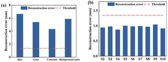
Figure 11.
Detection results of sensor failure. (a) S1 in four sensor failure cases; (b) other sensors.
The elastic moduli of the damaged area elements in Figure 7 are decreased by 5, 15, and 25%, respectively, and the other parameters of the structure are the same as those in the above study. Signal reconstruction was performed for each damage sample using the S-GRU NN trained on healthy structural data. An example of a set of reconstruction errors is shown in Figure 12, and four sensors (S4–S7) are seen to have reconstruction errors that exceed the threshold. These four sensors are located near the damage location. The detection results have an obvious relationship with the local damage to the structure.
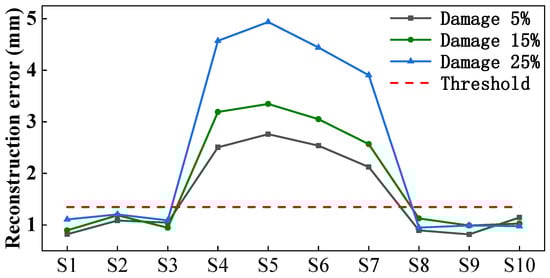
Figure 12.
Detection results of structural damage.
4.4. Isolation Performance Study of Sensor Failure and Structural Damage
Three sets of prediction data were designed to investigate the isolation performance of the models trained at different noise levels. The composition of the prediction data is presented in Table 1. Among them, the sensor failure sample was a random sensor failure and there are 25 samples for each type of sensor fault. The predicted results are for three types of events: healthy structure (H), sensor failure (F), and structural damage (S). The detection results for various prediction data are summarized in the confusion matrices in Figure 13. In the case of noise-free interference, the proposed framework can accurately isolate sensor faults and structural damage, even if the degree of structural damage is only 5%.

Table 1.
Composition of Prediction Samples.
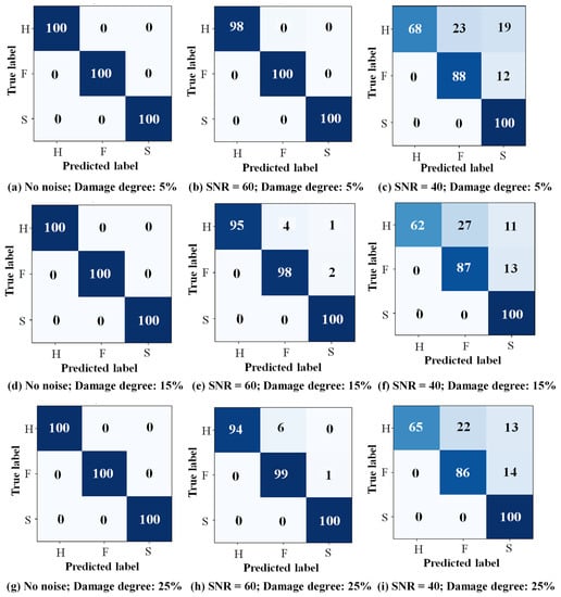
Figure 13.
Confusion matrices for different damage degrees and SNR values.
After adding white noise with an SNR of 60 to the measurement signal, a few healthy structure samples with a single sensor exceeding the threshold were identified as sensor faults. In the sensor failure samples, there were also individual normal sensors whose reconstruction errors exceeded the threshold. They were adjacent to the faulty sensor and were detected as structural damage.In the damaged samples, all sensors located near the damaged location are detected to be abnormal; therefore, they were correctly identified as structural damage.
When white noise with an SNR of 40 was added to the measurement signal, there were more normal sensors whose reconstruction errors exceeded the threshold, which led to the structure being incorrectly detected as a sensor failure or structural damage. However, the sensor reconstruction errors in all damaged areas exceeded the threshold, and the detection results of the damaged samples were still 100% accurate.
Comparing the isolation results under different SNR, it is found that when the signal is slightly polluted, the S-GRU NN model maintains a high accuracy. When the signal is heavily polluted, the reconstruction errors of some signals exceed the threshold; this reduces the accuracy of anomaly detection and affects the isolation of sensor faults and structural damage. It is worth noting that in the samples with structural damages, some of the sensor reconstruction errors located at undamaged locations also exceeded the threshold value. Because all sensors located near the damaged location exceeded the threshold value, the identification result was structural damage. Anomaly sensors located in undamaged locations should also be considered for practical applications.
To verify the superiority of the S-GRU NN model, we compared it with GRU, LSTM and CNN models in Section 4.1. The training dataset was the same as that of the S-GRU NN. According to the results in the literature [18], it is known that measurement noise mainly affects the identification of minor structural damage. Therefore, the prediction dataset was DS1 with two types of noise and no noise. We hoped that the proposed isolation strategy detected abnormal samples more accurately; thus, recall was used to evaluate the isolation performance of sensor faults and structural damage. The recall refers to the probability of being predicted as positive in all true-positive samples [45]. Figure 14 illustrates the recall rates of sensor faults and structural damages using the different models. The S-GRU NN is seen to show better recognition ability under different levels of noise interference. Furthermore, the calculation results were analyzed at two levels:
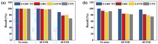
Figure 14.
Recall of faulty sensor and structural damage. (a) Faulty sensor; (b) structural damage.
- (1)
- In the case of no measurement noise, all four algorithms are used to accurately identify sensor faults, because the error between the measured and reconstructed signals due to sensor faults is large and far above the threshold value. However, when slightly noise is present in the measurement signal, the accuracy of detection of sensor faults is reduced. This is due to the fact that the noise causes the error between the measured and reconstructed values of the normal sensor to exceed the threshold value, and this sensor is adjacent to the fault sensor, thus the structure is incorrectly identified as a damaged state. By comparing the recall of the four algorithms, it can be found that S-GRU NN has better detection performance in noisy environments, which is due to the fact that the S-GRU NN can better capture the local features of the signal in noisy environments. The relatively small error between the reconstructed and measured signals, effectively avoiding the problem of difficulty in identifying sensor faults and structural damage in isolated frameworks due to noise.
- (2)
- With the increase of noise level, the recognition accuracy of all three comparison algorithms for structural damage showed a significant decrease. On the contrary, S-GRU NN still has good recognition accuracy even at the noise level of 40 SNR. This is due to the difficulty of GRU, LSTM, and CNN to effectively learn the local features of the signal in the noisy training data during the model training process, resulting in the reconstructed signal based on the trained model still has a large error with the true signal, and the calculated threshold is relatively high. When the structure showed light damage, the error between the measured damage signal and the reconstructed signal was relatively small and did not exceed the threshold value, thus incorrectly identifying the light damage signal as a healthy signal. However, the unique structure of S-GRU NN makes it have better reconstruction performance in noisy environment, and the calculated threshold can reflect the health status of the structure more realistically. The recall of S-GRU NN for the identification of slight structural damage and sensor failure is 100% and 86%, respectively, even under the noise disturbance of 40 SNR, which is sufficient to show the good robustness of the proposed method under different environmental noise. We can conclude that the method proposed in this study is sensitive to structural damage but insensitive to noise.
5. Experimental Verification
In this section, the 4-layer steel frame structure model illustrated in Figure 15 was used as the research object to confirm the accuracy of the proposed isolation framework. The steel frame construction column had a height of 0.8 m and each floor had a height of 0.2 m. The length of the beam was 0.35 m. The cross-section of the column and beam was 50 × 5 mm, with a mass density of 7850 kg/m. They are connected to adjacent structural members using angle steel and two bolts at both ends. The bottom of the column was fixed on an electromagnetic shaking table using angle steel bolts. The excitation of the electromagnetic shaker is a horizontal sinusoidal acceleration time course with a frequency of 50 Hz and an amplitude varying from 0–2.5 mm, and the direction is transverse to the beam. Eight acceleration sensors (S1–S8) are attached to the columns on each floor to capture the horizontal response of the structure. The sensors were located 30 mm below the top of each column, as shown in Figure 15. In addition, an acceleration sensor (S9) was attached to the edge of the shaking table to capture the input acceleration of the structure. The damage was simulated by removing a part of the material at a position of 50 mm in the middle of the column. The widths removed were 5, 15, and 25 mm, which simulated a column bending stiffness reduction of 10, 30, and 50%, respectively.
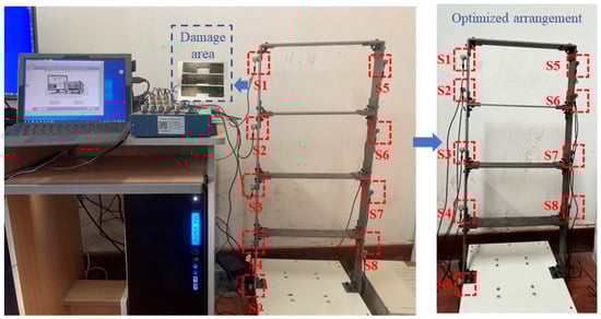
Figure 15.
Four layers of steel frame structure and the placement of acceleration sensors.
5.1. Data Preparation
In order to make the measured data include more environmental changes, we collected the dynamic response of the healthy structure and the unit damaged structure at different temperatures in five days by referring to the method in the literature [5]. The sampling frequency is 200 Hz. The measurement signal of S9 was used as the input data of the S-GRU NN model, and the output data of the model were the measurement signals of S1–S8. The measured signals of each sensor were segmented with every 2000 sampling points, and the datasets were then formed. Five hundred data samples of the healthy structure were selected, of which 80% were used as the training dataset and 20% as the validation dataset. All samples were prepared according to the format required by S-GRU NN. Because the stack size used by S-GRU NN is five, the input and output sizes of the training dataset were [400, 400, and 5] and [400, 400, and 8], respectively, and the input and output sizes of the validation dataset were [100, 400, and 5] and [100, 400, and 8], respectively. The other network parameters are the same as those described in Section 4.1. The training and validation datasets were sent to the S-GRU NN for learning and training of sensor signal reconstruction, and subsequently the threshold was calculated.
The prediction dataset consists of three parts: (1) a dataset of 50 healthy structures; (2) a dataset of structures with damage elements, with 50 samples for each degree of damage. (3) The sensor fault dataset was simulated using the method described in Section 3.1, where four types of sensor faults occurred at S1, and there are 50 samples for each fault type. It is worth noting that the sensor failure model used in this paper has been shown to be similar to the actual sensor failure states and has been widely used in experimental studies of sensor failures [28,30,31]. The LSTM, GRU, and CNN models in Section 4.1 were again used to compare with the proposed method.
5.2. Reconstruction Results
An example of the reconstructed responses obtained by the different methods is shown in Figure 16. The relative error of S-GRU NN reconstruction signal is 11.2%, while the relative errors of GRU, LSTM, and CNN reconstruction signals are 15.8, 18.5 and 19.0%, respectively. It can be found from Figure 16c,d that the reconstructed signals from the three compared models have a larger error in the maximum magnitude, which has a great response to the damage detection of the structure. However, as shown in Figure 16a, the unique network structure allows the S-GRU NN to learn more detailed features from the response signal, and the reconstructed signal is closer to the true response.
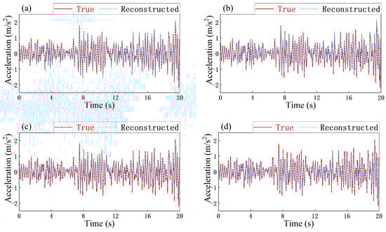
Figure 16.
Comparison of reconstructed signal and true signal. (a) S-GRU NN; (b) GRU; (c) LSTM; (d) CNN.
5.3. Sensor Failure and Structural Damage Isolation Framework Analysis
The reconstruction error of the prediction dataset is shown in Figure 17, Figure 18 and Figure 19. Figure 17 shows the sensor signal reconstruction error for each prediction sample of the healthy structure. Owing to the different output data of the different sensors, the reconstruction performance of the S-GRU NN was different. However, the threshold proposed in this study considers the maximum error of all sensors in the monitoring system, and therefore avoids the situation of “false positive” in the detection results. Figure 18 shows the reconstruction error of the sensor fault samples. The reconstruction errors of the sensor fault samples far exceed the threshold, which verifies that the isolation method proposed in this study effectively detects sensor faults. Figure 19 shows the detection results for structures with different degrees of damage. For 30 and 50% of structural damage scenarios, S1 and S2 correctly display that the data exceeds the threshold. For 10% of structural damage scenarios, only three samples did not exceed the threshold. The locations of S1 and S2 were very near to the damage location. S3 was also close to the damaged area, and the reconstruction errors of some samples also exceeded the card threshold.
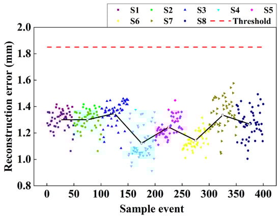
Figure 17.
Detection results of healthy structures.
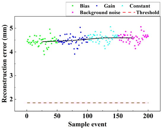
Figure 18.
Detection results of four faults in S1.
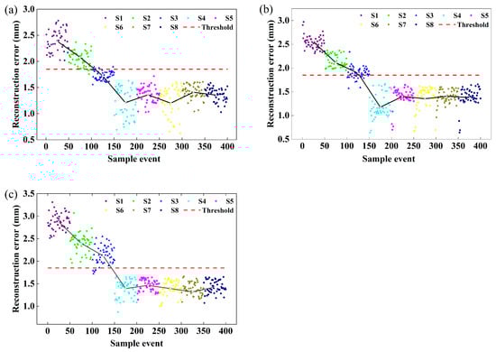
Figure 19.
Detection results with different degrees of damage. (a) 10% damage degree; (b) 30% damage degree; (c) 50% damage degree.
The GRU, LSTM, and CNN models in Section 4.1 were used to compare with the S-GRU NN and recall was used to measure the isolation performance of the framework using different algorithms. The results are shown in Figure 20, and it can be found that all four frameworks can accurately detect sensor failures and structures with 50% damage, due to the large error between the measured and reconstructed signals in both cases. However, when the structural damage is low, the S-GRU NN can detect more damage samples because of its better reconstruction accuracy and robustness. Therefore, we can conclude that the isolation method based on the S-GRU NN performed better.
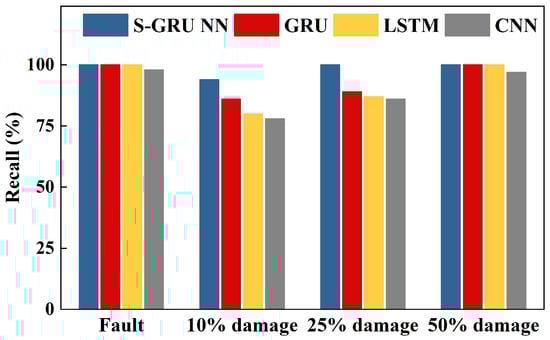
Figure 20.
Recall of detection results.
5.4. Sensor Arrangement Location Analysis
It can be found in Figure 19 that when the damage degree of the structure is 10%, the reconstruction errors of S2 do not all exceed the threshold. This may be because S2 was not on the same layer as the damaged area. When the structure was only slightly damaged, the acceleration changes little before and after the damage. It is worth noting that, the placement of the sensors plays a crucial role in the quality of the monitored information [46,47,48]. In order to improve the accuracy for damage identification of steel frame structures, we optimized the sensor placement based on the structural damage recognition results, as shown in Figure 15. Then, the response signals of the structure in the healthy state were re-collected to form the training and validation data, and the response signals of the structure in the 10% damage state were collected to form the prediction data. The structure of the dataset is the same as in the previous experiments. Figure 21 shows the results of structural damage detection using the proposed framework. It can be found that the reconstruction error of both S1 and S2 exceeds the threshold value, thus the identification result is that structural damage has occurred near S1 and S2. It can be concluded that the recognition accuracy of the proposed framework for slight structural damage can be improved after the optimization of the sensor placement of the structure.
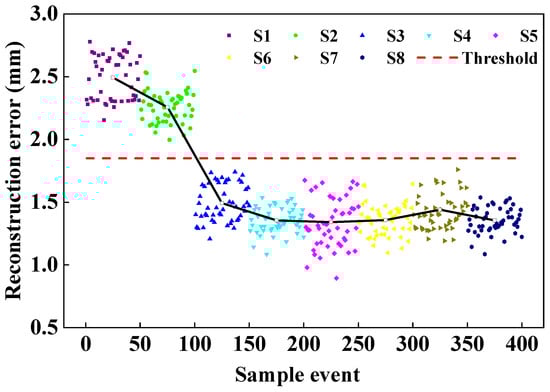
Figure 21.
Damage recognition results after sensor arrangement optimization.
6. Conclusions
A new isolation framework for sensor failures and structural damage considering measurement noise is proposed. This framework consists of three main modules: signal reconstruction, anomaly monitoring, and anomaly isolation. A S-GRU NN was defined to improve the performance of the signal reconstruction learning model. To improve the robustness of the model, a regularization term is used in the loss function of the model. An anomaly detection threshold was proposed based on the box-plot of the reconstruction error. To isolate sensor faults and structural damages, an isolation strategy was proposed based on the fact that sensor faults can be located in one sensor, and that structural damage causes an abnormality in sensors near the damaged location. A numerical study of a three-span continuous beam structure was carried out to evaluate the accuracy and robustness of the proposed method, especially considering the effect of noise on measured data. An experimental study of a four-story steel frame was conducted to further verify the performance of the proposed framework. The results show that, unlike the classical GRU, LSTM, and CNN methods, the S-GRU NN method has better accuracy and robustness in isolating structural damage and sensor faults.
Compared with other methods, the S-GRU NN method has two significantly different characteristics which greatly improve the effectiveness and robustness of the neural network model for anomaly detection: (1) deep neural network structure with a unique stacked structure and more hidden layers to improve the accuracy of the network model; (2) the use of the loss function’s regularization term in training to enhance the robustness of the network model. The results show that this framework isolates sensor faults and structural damages more accurately, particularly in the case of slight structural damage or high measurement noise. S-GRU NN, as a nondestructive detection method, is trained using only structural response data in a healthy state, and can accurately identify structural damage and sensor failures even if the response data contains a large amount of environmental noise. However, a limitation of the model is that the training and prediction samples require similar load and environmental conditions. This framework can further use other vibration characteristics that are more sensitive to structural damage to determine the degree of structural damage. This will be investigated in future studies.
Author Contributions
Conceptualization, methodology, formal analysis, writing—original draft preparation, B.L.; software, data curation, Q.X.; validation, writing—review and editing, J.C.; funding acquisition, B.L., Q.X., J.C., J.L. and M.W. All authors have read and agreed to the published version of the manuscript.
Funding
This work is fnancially supported by the National Natural Science Foundation of China (Grant Nos. 52192672 and 52079025). These sources of fnancial support are gratefully acknowledged.
Institutional Review Board Statement
Not applicable.
Informed Consent Statement
Not applicable.
Data Availability Statement
The data presented in this study are available on request from the corresponding author.
Conflicts of Interest
The authors declare no conflict of interest.
Abbreviations
The following abbreviations are used in this manuscript:
| SHM | Structural health monitoring |
| S-GRU NN | Stacked-gated recurrent neural network |
| CNN | Convolutional neural network |
| RNN | Recurrent neural network |
| LSTM | long short-term memory |
| GRU | Gate recurrent units |
| MSE | Mean square error |
| FC | Fully connected |
| RMSE | Root-mean-square error |
| IQR | Interquartile range |
| ARE | Average reconstruction errors |
| SNR | Signal-to-noise ratio |
References
- Li, J.; Hong, H. A review of recent research advances on structural health monitoring in western australia. Struct. Monit. Maint. 2016, 3, 33–49. [Google Scholar] [CrossRef]
- Fang, Z.; Wang, Z.; Zhu, R.; Huang, H. Study on wind-induced response of transmission tower-line system under downburst wind. Buildings 2022, 12, 891. [Google Scholar] [CrossRef]
- Kullaa, J. Sensor validation using minimum mean square error estimation. Mech. Syst. Signal Proc. 2010, 24, 1444–1457. [Google Scholar] [CrossRef]
- Kullaa, J. Distinguishing between sensor fault, structural damage, and environmental or operational effects in structural health monitoring. Mech. Syst. Signal Proc. 2011, 2976–2989. [Google Scholar] [CrossRef]
- Ma, S.L.; Jiang, S.F.; Li, J. Structural damage detection considering sensor performance degradation and measurement noise effect. Measurement 2019, 131, 431–442. [Google Scholar] [CrossRef]
- Ge, Z.; Song, Z.; Gao, F. Review of recent research on data-based process monitoring. Ind. Eng. Chem. Res. 2013, 52, 3543–3562. [Google Scholar] [CrossRef]
- Yang, Z.; Yu, Z.; Xie, C.; Huang, Y. Application of Hilbert-Huang Transform to acoustic emission signal for burn feature extraction in surface grinding process. Measurement 2014, 47, 14–21. [Google Scholar] [CrossRef]
- Vosoughi, A.R.; Gerist, S. New hybrid FE-PSO-CGAs sensitivity base technique for damage detection of laminated composite beams. Compos. Struct. 2014, 118, 68–73. [Google Scholar] [CrossRef]
- Dunia, R.; Qin, S.J.; Edgar, T.F.; McAvoy, T.J. Identification of faulty sensors using principal component analysis. AICHE J. 1996, 42, 2797–2812. [Google Scholar] [CrossRef]
- Tharrault, Y.; Mourot, G.; Ragot, J. Fault detection and isolation with robust principal component analysis. Int. J. Appl. Math. Comput. Sci. 2008, 18, 429–442. [Google Scholar] [CrossRef] [Green Version]
- Sharifi, R.; Kim, Y.; Langari, R. Sensor fault isolation and detection of smart structures. Smart Mater. Struct. 2010, 19, 105001. [Google Scholar] [CrossRef]
- Behmanesh, I.; Moaveni, B. Accounting for environmental variability, modeling errors, and parameter estimation uncertainties in structural identification. J. Sound Vibr. 2016, 374, 92–100. [Google Scholar] [CrossRef] [Green Version]
- Lee, C.; Sang, W.C.; Lee, I.B. Sensor fault identification based on time-lagged PCA in dynamic processes. Chemom. Intell. Lab. Syst. 2004, 70, 165–178. [Google Scholar] [CrossRef]
- Huang, H.B.; Yi, T.H.; Li, H.N. Sensor fault diagnosis for structural health monitoring based on statistical hypothesis test and missing variable approach. J. Aerosp. Eng. 2017, 730, B4015003. [Google Scholar] [CrossRef]
- Cui, P.; Ju, X.; Liu, Y.; Li, D. Predicting and improving the waterlogging resilience of urban communities in China—A case study of Nanjing. Buildings 2022, 12, 901. [Google Scholar] [CrossRef]
- Fan, G.; Li, J.; Hao, H. Dynamic response reconstruction for structural health monitoring using densely connected convolutional networks. Struct. Health Monit. 2020, 20, 1475921720916881. [Google Scholar] [CrossRef]
- Yuan, Z.; Zhang, L.; Duan, L. A novel fusion diagnosis method for rotor system fault based on deep learning and multi-sourced heterogeneous monitoring data. Meas. Sci. Technol. 2018, 29, 115005. [Google Scholar] [CrossRef]
- Rosafalco, L.; Torzoni, M.; Manzoni, A.; Mariani, S.; Corigliano, A. Online structural health monitoring by model order reduction and deep learning algorithms. Comput. Struct. 2021, 255, 106604. [Google Scholar] [CrossRef]
- Liu, G.; Li, L.; Zhang, L.; Li, Q.; Law, S.S. Sensor faults classification for SHM systems using deep learning-based method with tsfresh features. Smart Mater. Struct. 2020, 29, 075005. [Google Scholar] [CrossRef]
- Niu, Z.; Yu, K.; Wu, X. Lstm-based vae-gan for time-series anomaly detection. Sensors 2020, 20, 3738. [Google Scholar] [CrossRef]
- Zhang, R.; Chen, Z.; Chen, S.; Zheng, J.; Büyüköztürk, O.; Sun, H. Deep long short-term memory networks for nonlinear structural seismic response prediction. Comput. Struct. 2019, 220, 55–68. [Google Scholar] [CrossRef]
- Ryu, S.; Noh, J.; Kim, H. Deep neural network based demand side short term load forecasting. Energies 2016, 10, 3. [Google Scholar] [CrossRef]
- Lin, T.Y.; Goyal, P.; Girshick, R.; He, K.; Dollár, P. Focal loss for dense object detection. IEEE Trans. Pattern Anal. Mach. Intell. 2017, 99, 2999–3007. [Google Scholar]
- Li, L.; Liu, G.; Zhang, L.; Li, Q. FS-LSTM-based sensor fault and structural dDamage isolation in SHM. IEEE Sens. J. 2020, 21, 3250–3259. [Google Scholar] [CrossRef]
- Le, T.; Kim, J.; Kim, H. Classification performance using gated recurrent unit recurrent neural network on energy disaggregation. In Proceedings of the International Conference on Machine Learning and Cybernetics, Jeju, Korea, 10–13 July 2016; pp. 105–110. [Google Scholar]
- Li, S.; Li, S.; Laima, S.; Li, H. Data-driven modeling of bridge buffeting in the time domain using long short-term memory network based on structural health monitoring. Control. Health Monit. 2021, 28, e2772. [Google Scholar] [CrossRef]
- Srivastava, N.; Hinton, G.; Krizhevsky, A.; Sutskever, I.; Salakhutdinov, R. Dropout: Asimple way to prevent neural networks from overfitting. J. Mach. Learn. Res. 2014, 15, 1929–1958. [Google Scholar]
- Rozsa, A.; Gunther, M.; Boult, T.E. Towards robust deep neural networks with BANG. arXiv 2016, arXiv:1612.00138. [Google Scholar]
- Kerschen, G. Sensor validation using principal component analysis. Smart Mater. Struct. 2005, 14, 36–42. [Google Scholar] [CrossRef]
- Yi, T.H.; Huang, H.B.; Li, H.N. Development of sensor validation methodologies for structural health monitoring: A comprehensive review. Measurement 2017, 109, 200–214. [Google Scholar] [CrossRef]
- Malluhi, B.; Nounou, H.; Nounou, M. Enhanced Multiscale Principal Component Analysis for Improved Sensor Fault Detection and Isolation. Sensors 2022, 25, 5564. [Google Scholar] [CrossRef]
- Vad, V.; Cedrim, D.; Busch, W.; Filzmoser, P.; Viola, I. Generalized box-plot for root growth ensembles. BMC Bioinform. 2017, 18, 65. [Google Scholar] [CrossRef] [PubMed] [Green Version]
- Abubaker, M. Data mining applications in understanding electricity consumers’ behavior: A casestudy of Tulkarm district, Palestine. Energies 2019, 12, 4287. [Google Scholar] [CrossRef] [Green Version]
- Pan, C.; Yu, L. Sparse regularization-based damage detection in a bridge subjected to unknown moving forces. J. Civ. Struct. Health 2019, 9, 425–438. [Google Scholar] [CrossRef]
- Dang, H.V.; Raza, M.; Nguyen, T.V.; Bui-Tien, T.; Nguyen, H.X. Deep learning-based detection of structural damage using time-series data. Struct. Infrastruct. E. 2021, 17, 1474–1493. [Google Scholar] [CrossRef]
- Fan, G.; Li, J.; Hao, H.; Xin, Y. Data driven structural dynamic response reconstruction using segment based generative adversarial networks. Eng. Struct. 2021, 234, 111970. [Google Scholar] [CrossRef]
- Li, H.; Liu, H.; Ji, H.; Zhang, S.; Li, P. Ultra-short-term load demand forecast model framework based on deep learning. Energies 2020, 13, 4900. [Google Scholar] [CrossRef]
- Zou, J.Z.; Yang, J.X.; Wang, G.P.; Tang, Y.L.; Yu, C.S. Bridge structural damage identification based on parallel CNN-GRU. IOP Conf. Ser. Earth Environ. Sci. 2021, 626, 012017. [Google Scholar] [CrossRef]
- Son, H.; Pham, V.T.; Jang, Y.; Kim, S.E. Damage localization and severity assessment of a cable-stayed bridge using a message passing neural network. Sensors 2021, 21, 3118. [Google Scholar] [CrossRef]
- Li, Y.; Bao, T.; Gao, Z.; Shu, X.; Zhang, K.; Xie, L.; Zhang, Z. A new dam structural response estimation paradigm powered by deep learning and transfer learning techniques. Struct. Health Monit. 2022, 21, 770–787. [Google Scholar] [CrossRef]
- Glorot, X.; Bengio, Y. Understanding the difficulty of training deep feedforward neural networks. In Proceedings of the Thirteenth International Conference on Artificial Intelligence and Statistics, Sardinia, Italy, 13–15 May 2010; pp. 249–256. [Google Scholar]
- Pedregosa, F.; Varoquaux, G.; Gramfort, A.; Michel, V.; Thirion, B.; Grisel, O.; Blondel, M.; Prettenhofer, P.; Weiss, R.; Dubourg, V.; et al. Scikit-learn: Machine learning in Python. J. Mach. Learn Res. 2011, 12, 2825–2830. [Google Scholar]
- Meng, Q.; Chen, W.; Wang, Y.; Ma, Z.M.; Liu, T.Y. Convergence analysis of distributed stochastic gradient descent with shuffling. arXiv 2017, arXiv:1709.10432. [Google Scholar] [CrossRef] [Green Version]
- D’Alessandro, A.; Vitale, G.; Scudero, S.; D’Anna, R.; Costanza, A.; Fagiolini, A.; Greco, L. Characterization of mems accelerometer self-noise by means of psd and allan variance analysis. In Proceedings of the 7th IEEE International Workshop on Advances in Sensors and Interfaces IWASI, Vieste, Italy, 15–16 June 2017; pp. 159–164. [Google Scholar]
- Su, Y.; Zhao, Y.; Niu, C.; Liu, R.; Sun, W.; Pei, D. Robust anomaly detection for multivariate time series through stochastic recurrent neural network. In Proceedings of the 25th ACM SIGKDD International Conference on Knowledge Discovery & Data Mining, Anchorage, AK, USA, 4–8 August 2019; pp. 2828–2837. [Google Scholar]
- Yuen, K.V.; Kuok, S.C. Efficient Bayesian sensor placement algorithm for structural identification: A general approach for multi-type sensory systems. Earthq. Eng. Struct. D 2015, 44, 757–774. [Google Scholar] [CrossRef]
- Yi, T.H.; Li, H.N.; Zhang, X.D. Health monitoring sensor placement optimization for Canton Tower using immune monkey algorithm. Struct. Control Health 2015, 22, 123–138. [Google Scholar] [CrossRef]
- Ismail, Z.; Mustapha, S.; Fakih, M.A.; Tarhini, H. Sensor placement optimization on complex and large metallic and composite structures. Struct. Health Monit. 2020, 19, 262–280. [Google Scholar] [CrossRef]
Publisher’s Note: MDPI stays neutral with regard to jurisdictional claims in published maps and institutional affiliations. |
© 2022 by the authors. Licensee MDPI, Basel, Switzerland. This article is an open access article distributed under the terms and conditions of the Creative Commons Attribution (CC BY) license (https://creativecommons.org/licenses/by/4.0/).