Improved Metaheuristic Algorithm Based Finite Element Model Updating of a Hybrid Girder Cable-Stayed Railway Bridge

Abstract

This study proposes a generally applicable improvement strategy for metaheuristic algorithms, improving the algorithm’s accuracy and local convergence in finite element (FE) model updating. Based on the idea of “survival of the fittest” in biological evolution, the improvement strategy introduces random crossover and mutation operators into metaheuristic algorithms to improve the accuracy and stability of the solution. The effectiveness of the improvement strategy with three typical metaheuristic algorithms was comprehensively tested by benchmark functions and numerical simulations of a space truss structure. Meanwhile, the initial FE model of a railway hybrid girder cable-stayed bridge was updated to examine the effect of the improved metaheuristic algorithm within the FE model, updating for complex engineering structures. The results show that the accuracy and stability of the improved metaheuristic algorithm were improved by this process. After the initial FE model of the hybrid girder cable-stayed bridge was updated, the calculated frequencies and displacements were closer to the measured values, better representing the actual structure, and showing that this process can be used for baseline FE models of bridges.

1. Introduction

Due to material performance degradation, overloading, corrosive environments, and other effects, the performance of a bridge structure will gradually degrade, leading to potential safety hazards. In August 2008, the I-35W Bridge in the United States suddenly collapsed during rush hour, resulting in 13 deaths and 145 injuries [1]. In April 1987, the Schoharie Creek Bridge in New York, USA, collapsed, resulting in 10 deaths [2]. To avoid bridge accidents, structural health monitoring and condition assessments are usually implemented to evaluate the technical condition of existing bridge structures. A baseline finite element (FE) model, which can reflect the structural behavior of the actual bridge, is widely used in bridge condition assessment. However, due to the simplifications in FE modeling and the uncertainties in material properties, and also the errors of boundary conditions, the initial FE model established according to the design drawings usually fails to represent the actual bridge. Thus, updating the initial FE model, called FE model updating, according to the experimentally measured results, is necessary [3,4,5,6]. Many studies regarding FE model updating have been published in the past decade. A detailed overview of FE model updating can be found in reference [7].

FE model updating is essentially defined as an optimization problem with an objective function, which is usually expressed by the discrepancies between FE-calculated structural responses (such as displacement and modal parameters) and the experimentally measured ones. The objective function of bridge FE model updating usually has the characteristics of multi-dimensionality, high nonlinearity, and multiple local extremes. Traditional optimization algorithms, such as gradient-based algorithms [8,9] and the Newton iteration method [10,11], easily fall into the local optimum when dealing with such optimization problems. Consequently, these algorithms find it difficult to obtain the global optimal solution of the objective function. In recent years, metaheuristic algorithms, such as particle swarm optimization algorithm (PSO) [12,13], bee colony algorithm (BCA) [14,15], ant colony algorithm [16,17], and gravitational search algorithm (GSA) [18,19], which are based on intelligent optimization theory, have been developed and widely used in multidisciplinary optimization problems. For example, Huang et al. [20] proposed a nondestructive global damage identification method based on vibration and successfully applied the method to three-span continuous beams and two-span steel grids in multiple damage scenarios. Huang et al. [21] proposed a structural damage identification method based on support vector machine (SVM) and moth-flame optimization (MFO) and successfully applied the method to a simply-supported beam and an actual bridge engineering example. It is generally accepted that, compared with traditional algorithms, metaheuristic algorithms have certain advantages in dealing with nonlinear and multi-extremum issues [22].

Although the metaheuristic algorithm is superior to traditional optimization algorithms to a certain extent, it is still limited by the characteristics of the algorithm itself [22,23]. There is a contradiction between the population’s diversity and the algorithm’s convergence speed in the search process. Especially in actual engineering cases, most of them have multiple extreme points, and the algorithm easily falls into the local optimum. Therefore, the metaheuristic algorithm’s performance needs to be improved. On this issue, some relevant research has been conducted. Ding et al. [24] introduced two local search strategies into the artificial bee colony algorithm to improve the identification accuracy of the algorithm. The authors proved that the improved algorithm could provide more accurate results using incomplete modal data through a case study of a real structure. To solve the problem of premature convergence in the ant colony algorithm, Yang [25] utilized step control parameters to improve the performance of the standard ant colony algorithm. Their study shows that the improved ant colony algorithm can provide better results. Jiang et al. [26] divided the population into several subpopulations by combining the concepts of PSO, competitive evolution, and complex shuffle to solve the local convergence problem. Each subpopulation independently executes the standard PSO, and after several iterations the subpopulations are mixed to ensure information sharing. The authors applied the improved algorithm to hydrological model updating and proved that the improved PSO could jump out the local minimums. Marzband et al. [27] proposed an optimization method based on GSA. A control parameter was added to the GSA algorithm to adjust the searching ability of the algorithm in later stages to avoid premature inaccuracies. The improved GSA algorithm was applied to a real-time energy management system of the microgrid to achieve the highest efficiency, improve the efficiency of economic dispatch, and obtain the best performance. The above studies aim to optimize and improve the algorithm parameters of a particular algorithm, while some other studies integrate two optimization algorithms to improve the algorithms’ performance. Wang et al. [28] introduced the artificial fish swarm algorithm to construct an entropy path planning model of the hybrid ant colony and artificial fish swarm algorithm to improve the convergence speed and accuracy of the algorithm. Based on the combination of GSA and PSO, Hu et al. [29] changed the constant acceleration coefficient into an exponential function and proposed an improved PSO-GSA algorithm to solve the robot’s surface water quality and movement direction. The results showed that the hybrid algorithm can improve the local convergence problem of the standard algorithm. Huang et al. [30] introduced Levy-flight in the whale optimization algorithm to increase the diversity of the population to solve the problems of premature maturity and slow convergence of the whale optimization algorithm. The improved whale optimization algorithm was applied to the damage identification of three examples. To improve the sampling efficiency of standard Metropolis-Hastings (MH), Luo et al. [31] introduced the particle position update mechanism of PSO into the MH algorithm and formed the MH-PSO hybrid Markov chain Monte Carlo sampling method. The sampling method was successfully applied to the Bayesian model updating of a cantilever beam and ASCE benchmark frame.

The abovementioned improvement strategy is only applicable to one metaheuristic algorithm. Most metaheuristic algorithms receive inspiration from random phenomena and swarm intelligence behaviors in nature, and the random search module is introduced based on the heuristic algorithm, making the metaheuristic algorithm more widely applicable. This study proposes an improvement strategy that is generally applicable to different metaheuristic algorithms to improve the metaheuristic algorithm’s local convergence and search accuracy. Based on the idea of survival of the fittest in biological evolution, the improvement strategy adds random crossover and mutation calculations within the standard metaheuristic algorithm to improve the position of the population in the search space to jump out of the local optimum and improve the search accuracy.

The framework of this paper is as follows. Section 2 introduces the basic theory of FE model updating, based on the kriging surrogate model. Section 3 presents the metaheuristic algorithm and the improvement strategy and verifies the results of the improvement through benchmark functions. Section 4 numerically investigates the performance of the improvement strategy through FE model updating of a space truss structure. 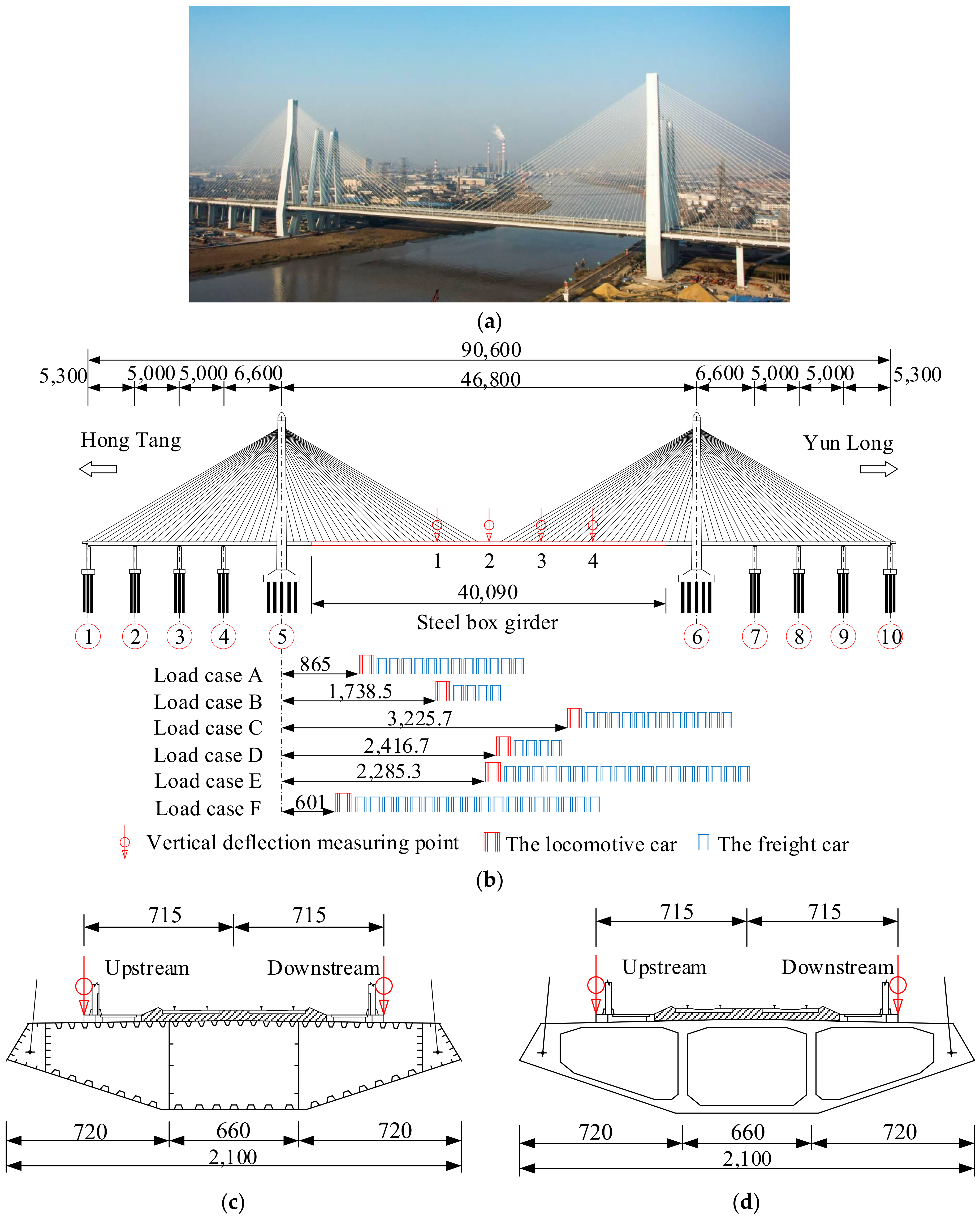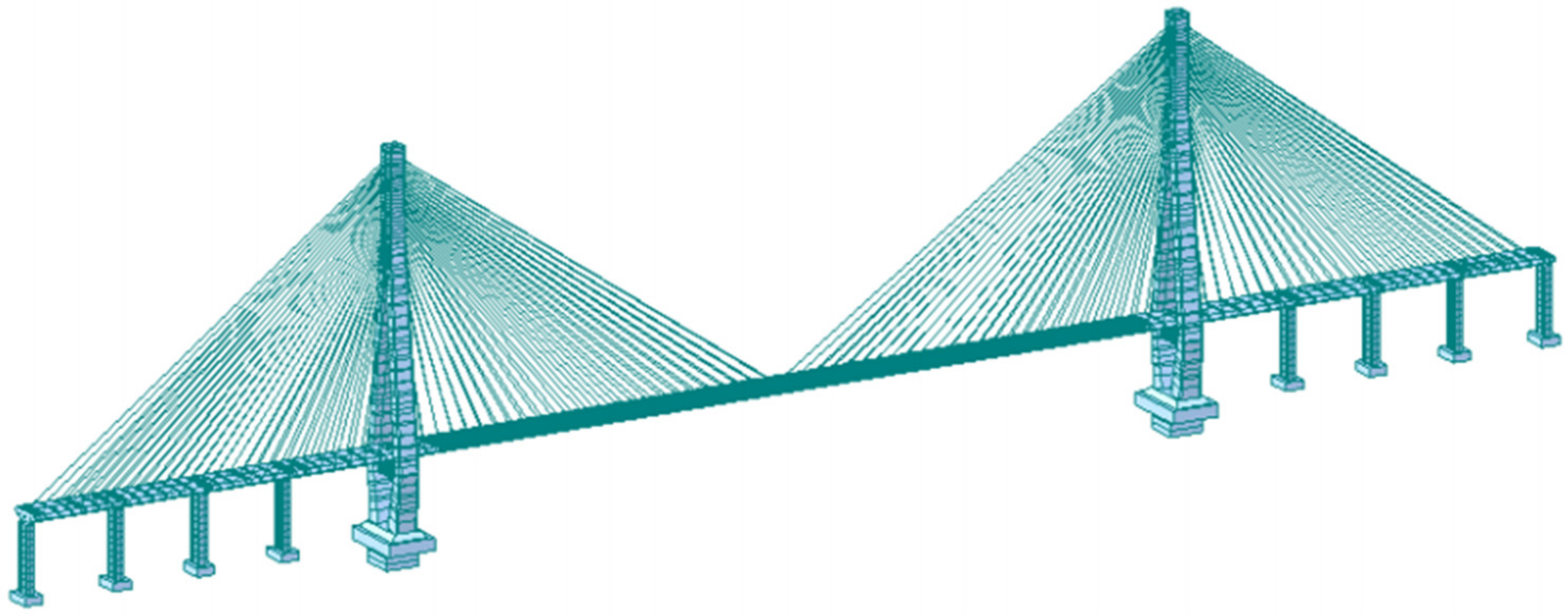In Section 5, the FE model updating of a full-scale long-span hybrid girder cable-stayed railway bridge is implemented based on the proposed algorithm. The basic information of the bridge, the in situ testing, the initial FE model, the kriging model, and the updating results, using the improved metaheuristic algorithms, are introduced and discussed. The conclusions are made in the final section.

2. Model Updating Assisted with the Kriging Model

The essence of FE model updating is to reduce the error between the FE-calculated response values and the experimentally measured ones by updating the structural design parameters in the FE model. Therefore, the objective function $J(x)$ can be defined as:

$$\left.\begin{array}{l}J(x)=\min {\displaystyle \sum _{i=1}^m{\alpha }_i{r}_i}(x)\\ \mathrm{s}.\mathrm{t}.x_m^{\min }\le x_m\le x_m^{\max }\end{array}\right\}$$

(1)

where x is the design parameter to be updated; $r_i(x)$ is the residual function between the calculated value and the measured value of the i-th type of structural response; m is the number of the kinds of structural responses considered in model updating; ${\alpha }_i$ is the weighting coefficient of the i-th residual function; and $x_m^{\max }$ and $x_m^{\min }$ are the upper and lower bounds of the m-th design parameter to be updated, respectively.

The iterative method is widely used to obtain the minimum value of the objective function in a design space. However, due to the implicit functional relationship between the structural response and the design parameters, the FE model calculates the residual function in each iteration, which is very time-consuming, especially for complex FE models of bridge structures. Surrogate models, such as polynomial response surface, radial basis function, and the kriging model, have been used for model updating to improve calculation efficiency. Study [32] has shown that the kriging model predicts the value of each point in the design space and gives each point’s prediction error. Therefore, the kriging model was selected as the surrogate model in FE model updating to save computational cost. The primary process of FE model updating based on the kriging model can be divided into three steps. Firstly, the data samples of structural responses and design parameters are generated by the design of the experiment with the aid of the initial FE model. The commonly used experimental design methods include central composite design, D-optimal design, uniform design, and latin hypercube design. Then, the kriging model is established based on the data samples using mathematical regression. An accuracy test of the kriging model is usually evaluated before it is applied within FE model updating. Finally, the optimization algorithm is applied to find the minimum of the objective function in the design space.

The kriging model comprises a deterministic regression model and a random process. The structural response matrix $\mathit{Y}(\mathit{x})$ can be expressed as the function of the design parameter x in the kriging model, and the formula is represented by:

$$\mathit{Y}(\mathit{x})={\displaystyle \sum _{j=1}^n{\beta }_j{f}_j(\mathit{x})+\mathit{Z}(\mathit{x})}$$

(2)

where n is the number of structural responses; ${\displaystyle \sum _{j=1}^n{\beta }_j{f}_j(\mathit{x})}$ is the polynomial regression model, which approximates the model at the global scale; ${\beta }_j$ is the regression coefficient; $f_j(\mathit{x})$ is a polynomial function of the structural design parameters; and $\mathit{Z}(\mathit{x})$ is a random process matrix with a mean value of 0 and a covariance of ${\sigma }^2$, which provides a local approximation of the model. The kriging model has been successfully applied to model updating, geological parameter analysis, and within multidisciplinary research fields [33,34,35,36]. A detailed description of the kriging model can be found therein.

3. Improvement Strategy of Metaheuristic Algorithm

3.1. Metaheuristic Algorithm

The metaheuristic algorithm improves on the heuristic algorithm, which combines random and local search algorithms. Metaheuristics are an iterative generation process; through the intelligent combination of different concepts, the process realizes the exploration and development of a search space by the heuristic algorithm. Learning strategies acquire and master information to discover near-optimal solutions in this process. Typical metaheuristic algorithms include GSA, simulated annealing algorithm (SA), genetic algorithm (GA), and PSO. GSA is taken as an example to illustrate the idea of a metaheuristic algorithm in this section.

GSA is an intelligent search algorithm that simulates the law of universal gravitation. Each particle in GSA can be regarded as an individual with its own position and moving speed. It can retain the optimal position that the particles have found so far and the global optimal position that all particles can find currently. In the standard GSA, the attraction $F_{ij}^d$ between particles i and j can be expressed as:

$$F_{ij}^d=G(t)\frac{M_{pi}(t)\times M_{ai}(t)}{R_{ij}(t)+\epsilon }(p_j^d(t)-p_i^d(t))$$

(3)

where $p_i^d(t)$ is the position of the i-th individual in d-dimensional space at time t; $M_{pi}(t)$ is the mass of individual i at time t; $M_{aj}(t)$ is the mass of individual at time t; ε is a small constant; and $R_{ij}(t)$ is the Euclidean distance between particles i and j, which can be expressed as:

$$R_{ij}(t)=‖p_i(t),p_j(t)‖$$

(4)

$G(t)$ represents the constant coefficient of universal gravitation at time t, which can be defined as:

$$G(t)=G_0{e}^{-\alpha \frac{t}{T}}$$

(5)

where $G_0$ represents the initial value of the constant coefficient; $\alpha$ denotes the descent coefficient; and T is the total number of iterations. Therefore, the resultant force $F_i^d$ of the i-th individual in the d-dimensional space can be expressed by:

$$F_i^d={\displaystyle \sum _{j=1,j\ne 1}^{N}rand\times F_{ij}^d}$$

(6)

where N is the number of particle populations and rand is a random number between 0 and 1. The acceleration $ac{c}_i^d(t)$ of a particle i at time t instant can be expressed as:

$$ac{c}_i^d(t)=\frac{F_i^d(t)}{M_{ii}(t)}$$

(7)

where $M_{ii}(t)$ is the inertial mass of the particle i at time t. The speed at which particles i move in d-dimensional space and the update of their position can be expressed as:

$$V_i^d(t+1)=rand\times V_i^d(t)+ac{c}_i^d(t)$$

(8)

$$p_i^d(t+1)=p_i^d(t)+V_i^d(t+1)$$

(9)

where $V_i^d(t)$ and $p_i^d(t)$ represent the moving speed and position of the t-th particle, respectively. The inertial mass of i-th particle $m_i(t)$ at the t-th time step can be expressed as:

$$m_i(t)=\frac{worst(t)-fi{t}_i(t)}{worst(t)-best(t)}$$

(10)

where $fi{t}_i(t)$ denotes the best solution of the individual at the t-th time step. $worst(t)$ and $best(t)$ denote the worst and best fitness of the individual in the population at the t-th time step, respectively. Assuming that the gravitational mass $M_{ai}$ and inertial mass of the individual $M_{pi}$ are equal to the mass of the individual $M_i$, it follows that:

$$M_{ai}=M_{pi}=M_i,i=1,2,\cdot \cdot \cdot ,N$$

(11)

$$M_i(t)=\frac{m_i(t)}{{\displaystyle \sum _{i=1}^N{m}_i(t)}}$$

(12)

It is known that when the particle’s fitness is greater, the mass of the particle will be more prominent, and its moving speed will be slower, which will continue to attract particles with poor fitness to move to the position with better fitness.

3.2. Improvement Strategy

As previously mentioned, the metaheuristic algorithm easily falls into local optimal values because of the limitation of the algorithm itself when the search reaches the later stage, thus reducing the search accuracy and efficiency. This study proposes an improvement strategy that is generally applicable to different metaheuristic algorithms. The proposed improvement strategy introduces random crossover and mutation into a standard metaheuristic algorithm, improving the algorithm’s searching ability at the later stage. The idea of using GA to improve the performance of the algorithm has already been adopted in multi-objective optimization; for examples of this, see Deb et al. [37] and Li and Zhang [38]. However, local convergence is a complex issue for metaheuristic algorithms. It is affected by many factors such as the algorithm’s parameters, the definition of the optimization problem, termination criterion, etc. Although the improvement strategy can improve the performance of the standard algorithm to a certain extent, the improvement strategy is not free from local convergence problems. The detailed procedure for the improvement is described as follows.

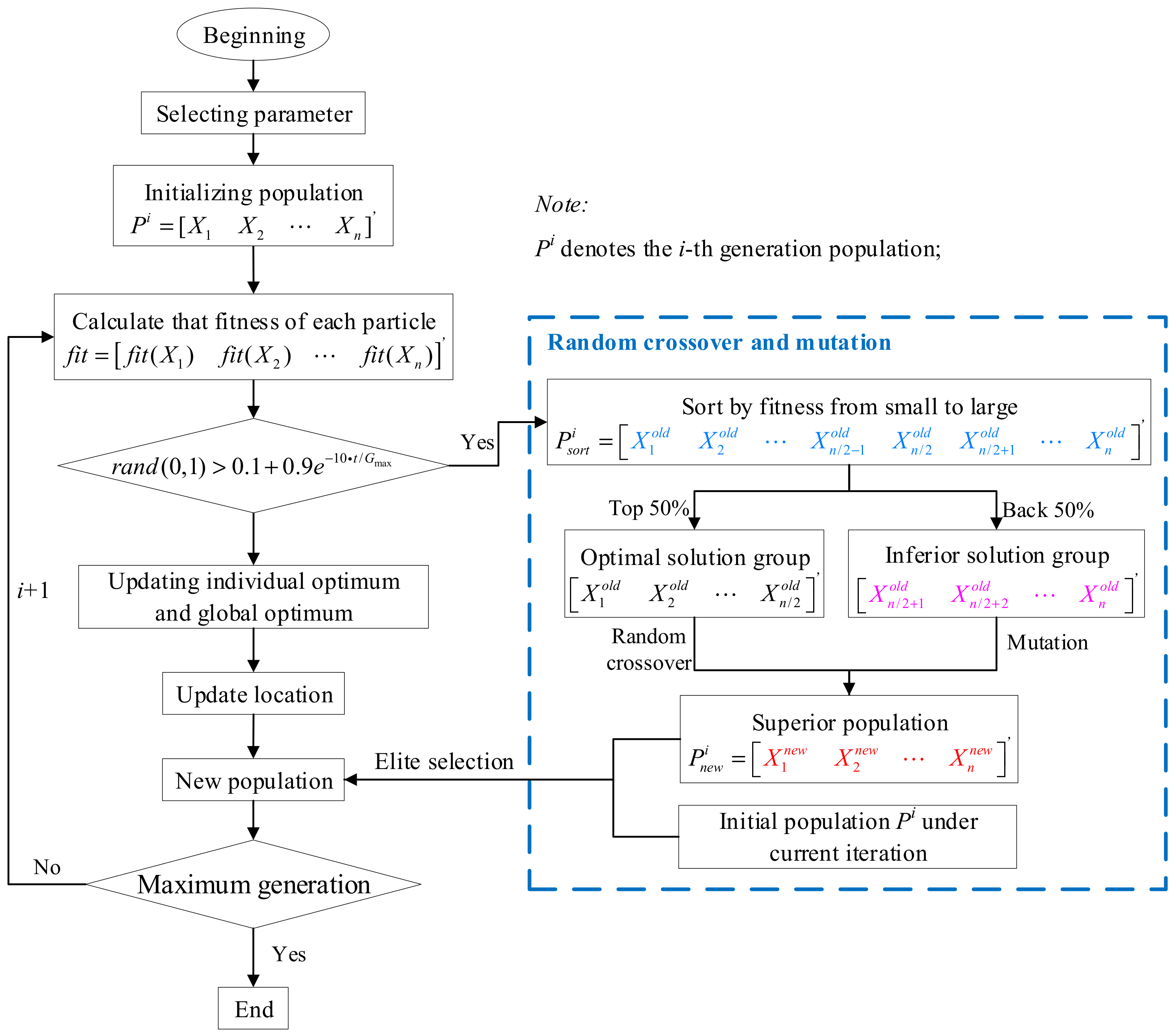
The proposed method firstly generates an initial population with the population number of $N$, calculating the fitness value $fit(t)$ of all particles and sorting the particles. Then, the algorithm divides the particles into optimal and inferior solution groups according to fitness values; the first 50% of the particles with better fitness values are regarded as the optimal solution group, and the last 50% of the particles with worse fitness are regarded as the inferior solution group. Since the individual particles of the optimal solution group are excellent, the random crossover operation is applied for the optimal solution group, which can retain the population information of the optimal solution group and ensure the algorithm’s search accuracy. However, inferior solutions require more remarkable changes to generate new offspring. The mutation operation is applied for the inferior solution group, which can enrich population diversity, help the metaheuristic algorithm to jump out of the local optimal solution, and improve the search ability in the later stage of the algorithm.

For example, all particles of PSO move in the direction of the particle with the best fitness value during optimization, resulting in a gradual decrease in the diversity of particles, with the particles often not being able to escape from the local optimal solution. In the case of the PSO algorithm falling into the local optimal solution, the mutation operation of the improvement strategy can enrich population diversity so that the algorithm can jump out of the local optimal solution and find the global optimal solution.

This study introduces a random judge condition to judge whether the algorithm entered into the later searching stage or not. If a random number rand(0, 1) in each generation satisfies the following condition, the random crossover and mutation are applied to the two particles group. The condition is:

$$rand(0,1)>0.1+0.9e^{-10·t/G_{\max }}$$

(13)

where G_max is the maximum generation; t is the current generation; and e is the natural index. It can be concluded from Equation (13) that with a generation’s increase, the probability of implementing random crossover and mutation operation also increases.

It is worth mentioning that the two particles for the random crossover operation in the improved algorithm are randomly selected, which can be expressed by:

$${\stackrel{⏜}{p}}_i{}^{\prime }=\eta {\widehat{p}}_{index1(i)}+(1-\eta ){\widehat{p}}_{index2(i)},i=1,2,3,\cdots ,\widehat{N}$$

(14)

where ${\stackrel{⏜}{p}}_i{}^{\prime }$ represents the offspring generated from the optimal solution set; ${\widehat{p}}_{index1(i)}$ and ${\widehat{p}}_{index2(i)}$ represent random particles without duplication in the optimal solution set; $index$ is an integer ranging from 1 to $\widehat{N}$; $\eta$ is a random number ranging from 0 to 1; $\widehat{N}$ represents the number of population particles within the optimal solution group; the size is $N/2$. The mutation operation is applied for the inferior solution group, which can be expressed as:

$${\widehat{p}}_i{}^{\prime \prime }=\left\{\begin{array}{l}{\tilde{p}}_i+({\tilde{p}}_i-p_{\max })\times f(t),rand>0.5\\ {\tilde{p}}_i+({\tilde{p}}_i-p_{\min })\times f(t),rand<0.5\end{array}\right.$$

(15)

where ${\stackrel{⏜}{p}}_i{}^{\prime \prime }$ represents the offspring generated from the inferior solution group; ${\tilde{p}}_i$ represents the i-th particle in the inferior solution group according to the fitness; $p_{\max }$ and $p_{\min }$, respectively, denote the upper and lower bound for all possible values of each particle, which are global variables; $f(t)=rand\times {(1-t/G_{\max })}^2$, rand represents the random number between 0 and 1; and $t$ represents the current number of iterations.

A new population ${\stackrel{⏜}{p}}_i{}^{\prime \prime \prime }$ is obtained by merging ${\stackrel{⏜}{p}}_i{}^{\prime }$ and ${\stackrel{⏜}{p}}_i{}^{\prime \prime }$, and the size of the new population ${\stackrel{⏜}{p}}_i{}^{\prime \prime \prime }$ is consistent with the size of the initial population. Then, the population ${\stackrel{⏜}{p}}_i{}^{\prime \prime \prime }$ is merged with the initial population to form an expanded population. The expanded population is rearranged according to the fitness, and finally, the optimal half-population is selected as a new iterative population for updating iteration.

3.3. Algorithm Procedure

The procedure of the improved algorithm is described as follows. Figure 1 shows the flow chart of the improved algorithm.

Step 1: Initialize the parameters of the algorithm;

Step 2: Randomly generate an initial population;

Step 3: Calculate the fitness of the initial population and initializing an individual optimal value and a global optimal value;

Step 4: Judge whether random crossover and mutation should be implemented or not. If $rand(0,1)>0.1+0.9e^{-10·t/G_{\max }}$, enter step 5, otherwise, enter step 7;

Step 5: Dividing the particles into two groups: optimal and inferior, according to the fitness values. The random crossover and mutation are respectively implemented in the optimal and inferior groups to generate new offspring;

Step 6: Elite selection. Merging the offspring generated by random crossover and mutation into one group further establishes an expanded population with the initial population under the current generation. Sorting the expanded population according to fitness and selecting the half of the population which has better fitness as the elite population to participate in the next iteration;

Step 7: Updating the velocity and position of the particles using Equations (8) and (9);

Step 8: Updating the individual optimal value and the global optimal value of particles;

Step 9: Judge whether that iteration termination standard is met; if the algorithm reaches the maximum iteration times, terminate the algorithm; otherwise, jump to step 3;

3.4. Benchmark Functions

To test the effectiveness of the improvement strategy, the performance of three typical metaheuristic algorithms, including PSO, GSA, SA, artificial fish swarm algorithm (AFSA), artificial ant colony (ABC) algorithm, and their respective improved versions, IPSO, IGSA, ISA, IAFSA, and IABC, are compared based on benchmark functions. Furthermore, to test the generality and effectiveness of the improved strategy, the PSOGA and the IPSO are compared based on benchmark functions. PSOGA [39] is a hybrid algorithm proposed by Kao and Zahara in 2008. At present, the PSOGA algorithm has been widely applied in the comparison of improvement strategies and optimization problems in the engineering field. The population size of all algorithms is set to 50, and the maximum number of iterations is 100 to ensure the comparability of each algorithm. For PSO, the learning factors $c_1$ and $c_2$ are 1.5 and 0.5, respectively, and the inertia constant is 0.726. These parameters are the default parameters of standard PSO and have been proved suitable for various optimization problems. For GSA, the universal gravitation coefficient is 10 and the descent coefficient is 20. For SA, the attenuation parameter is 0.95, the initial temperature is 50, and the final temperature is 0. For AFSA, the field of view is 0.025, the step size is 0.3, and the crowding factor is 0.1. For ABC, the number of observed bees and the number of employed bees take the same value of 50.

The two benchmark functions are the Ackley’s path function and the sum of different power function, represented by f₁ and f₂, respectively. The f₁ is a multimodal function that has several extreme points but only one global optimal point. The f₂ is a unimodal function. The objective functions f₁ and f₂ can be defined as:

$$f_1=-5\cdot e^{-0.2\sqrt{\frac{{\displaystyle \sum _{i=1}^n{x}_i^2}}{n}}}-e^{\frac{{\displaystyle \sum _{i=1}^n\cos }\left(2\pi \cdot x_i\right)}{n}}+5+e^1,i=1,2,\cdot \cdot \cdot ,10$$

(16)

$$f_2={\displaystyle \sum _{i=1}^d{\left|x_i\right|}^{i+1}},i=1,2,\cdot \cdot \cdot ,10$$

(17)

where x_i denotes the i-th design variable; and e is the natural index.

The dimensions of both functions are set as 2, and the corresponding function graphs are plotted in Figure 2a,b, respectively. The two functions are utilized to test the convergence accuracy of the algorithm and the ability to jump out of local optimal solution. The global optimal values of the two test functions are $x_i=0,(i=1:n),f(x)=0$. To eliminate the influence of randomness in the algorithm, each algorithm is independently run 100 times with MATLAB R2018a. The CPU is [email protected] GHz, and the memory size is 16 GB. The statistical results, including the mean value and standard deviation of the 100 independent runs, are employed to evaluate the searching accuracy and stability of each algorithm, respectively.

Table 1. The mean and standard deviation values obtained from different algorithms for benchmark functions.

Algorithm	f1		f2
	Mean	Standard Deviation	Mean	Standard Deviation
IGSA	5.50 × 10−2	7.43 × 10−3	2.72 × 10−6	9.43 × 10−6
GSA	6.71 × 10−1	1.83 × 10−2	6.77 × 10−6	2.53 × 10−5
IPSO	3.10 × 10−1	1.38 × 10−2	1.89 × 10−5	2.92 × 10−5
PSOGA	4.41 × 10−1	2.57 × 10−1	5.43 × 10−6	2.49 × 10−5
PSO	1.25	2.51 × 10−2	6.32 × 10−4	6.31 × 10−5
ISA	6.52 × 10−1	4.91 × 10−3	3.46 × 10−6	3.39 × 10−5
SA	8.22 × 10−1	6.58 × 10−3	6.51 × 10−5	2.27 × 10−4
IAFSA	5.74 × 10−1	9.01 × 10−3	3.15 × 10−5	3.52 × 10−5
AFSA	6.31 × 10−1	5.92 × 10−3	9.02 × 10−5	7.58 × 10−5
IABC	5.67 × 10−2	4.62 × 10−3	3.00 × 10−6	9.45 × 10−6
ABC	1.79	9.72 × 10−3	9.62 × 10−6	1.93 × 10−5

shows the mean and standard deviation of the two functions obtained from the 100 independent runs of the 5 algorithms. It can be seen that the mean and standard deviation values of both test functions obtained from the improved algorithms are smaller than those obtained from standard algorithms. For example, the mean and standard deviation values of f₁ obtained from standard GSA are 6.71 × 10⁻¹ and 1.83 × 10⁻², respectively, while corresponding values obtained from IGSA are 5.50 × 10⁻² and 7.43 × 10⁻³. This comparison indicates that the searching accuracy of IGSA is far better than GSA. Similar conclusions can be made for the other four algorithms. It can be seen from Table 1 that the mean and standard deviation of f₁ obtained from PSOGA are 4.41 × 10⁻¹ and 2.57 × 10⁻¹, respectively, while corresponding values obtained from IPSO are 3.10 × 10⁻¹ and 1.38 × 10⁻². From the comparison of the above results, it can be found that in the case of multiple local optimal solutions, IPSO has a greater probability of jumping out of the local optimal solution. In order to better demonstrate the generality of the improvement strategy, the following numerical and engineering cases mainly compare GSA, PSO, and SA and the corresponding improved algorithms.

Figure 3 shows the convergence curves of each algorithm for the two functions. The solid lines represent the convergence curves of the standard algorithms, while the dotted lines denote the convergence curves of the improved algorithms. It can be seen that compared with the standard algorithms, all improved algorithms have a higher capability to jump out of the local minimum and converge to a global minimum. For example, the standard GSA fell into a local minimum in generation 5, with an average fitness value of 1.2492 when searching the global minimum of f₁, whereas the IGSA reached a far smaller value of 0.3099. A similar situation can be found in the other two algorithms.

4. Numerical Simulation

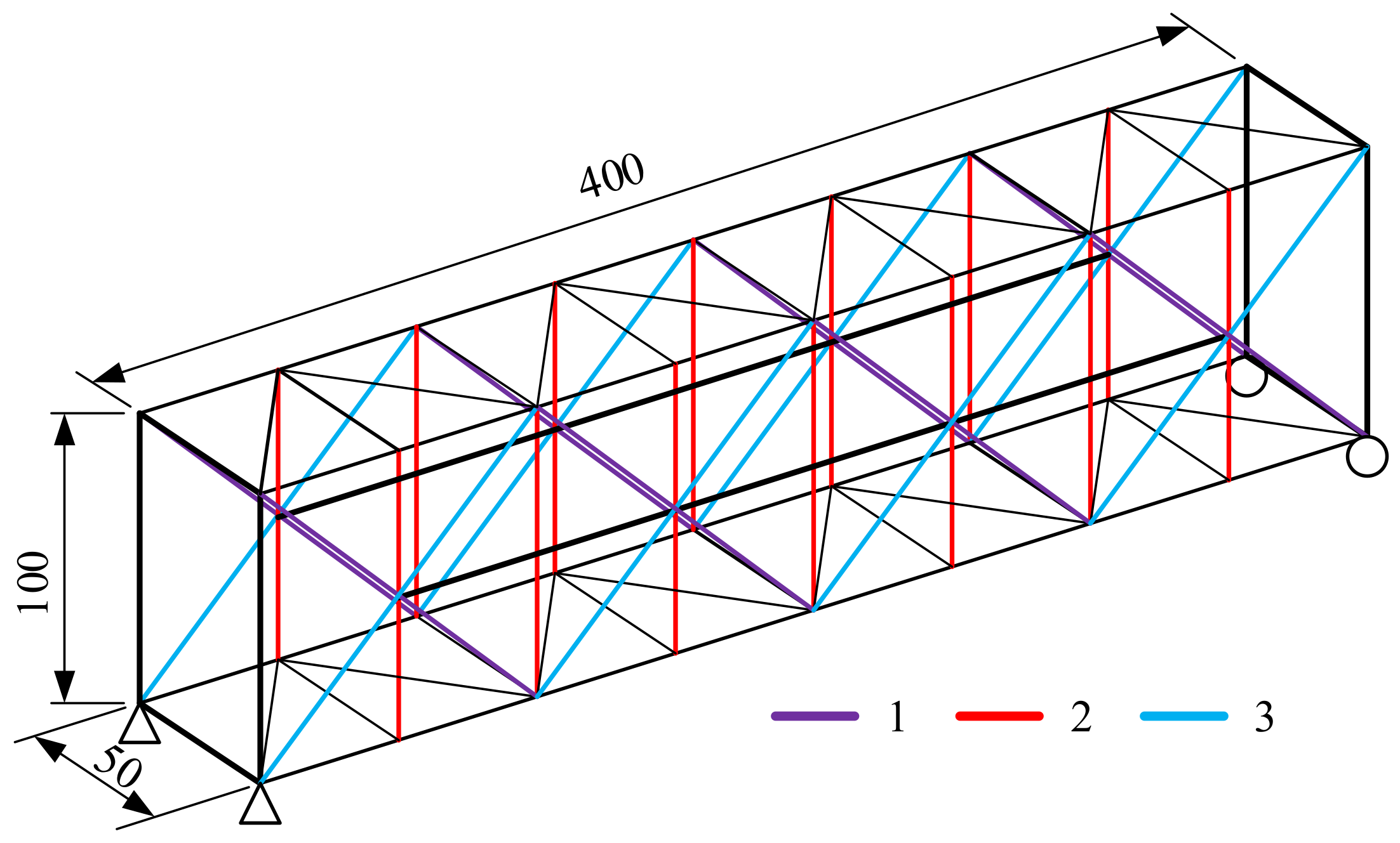
This section numerically updates the FE model of a simply supported space truss structure to test the effectiveness of the improvement strategy in FE model updating. Compared with the actual engineering structure, the damage location in the numerical example is known, and there is no updating parameter selection problem. Therefore, it can more accurately reflect the effectiveness of the improved heuristic algorithm. The truss structure is shown in Figure 4. The structural parameters are as follows: the span of the truss is 4 m, the height is 1 m, the elastic modulus of the material is set as 100 GPa, the density is 7850 kg/m³, and the section area of the beam element is 1.717 × 10⁻³ m². The FE model was established by ANSYS, and the beam element was used to simulate the truss members.

The truss’s diagonal members are divided into three groups according to the color, as illustrated in Figure 4. The elastic modulus of each group and the first six frequencies are taken as the design parameters and responses, respectively. The damage scenario is as follows: the elastic modulus of the first and second group of members is reduced by 30%, and the elastic modulus of the third group of members is increased by 30%. Figure 5 shows the first 6 mode shape of the truss.

To conveniently establish the kriging model, the relative value of the changed elastic modulus and the initial elastic modulus is taken as the design variable, and the sixth order frequency is taken as the response. The latin hypercube sampling method was used to design the experiment for the data samples of updating parameters. The three design parameters were sampled 36 times, and the sampling range of the parameters was set within ±30% of their initial values. Then the updating parameters were brought into the initial FE model to obtain the frequency. Finally, the kriging model was established by using the sample points as the input and the modal frequency response as the output.

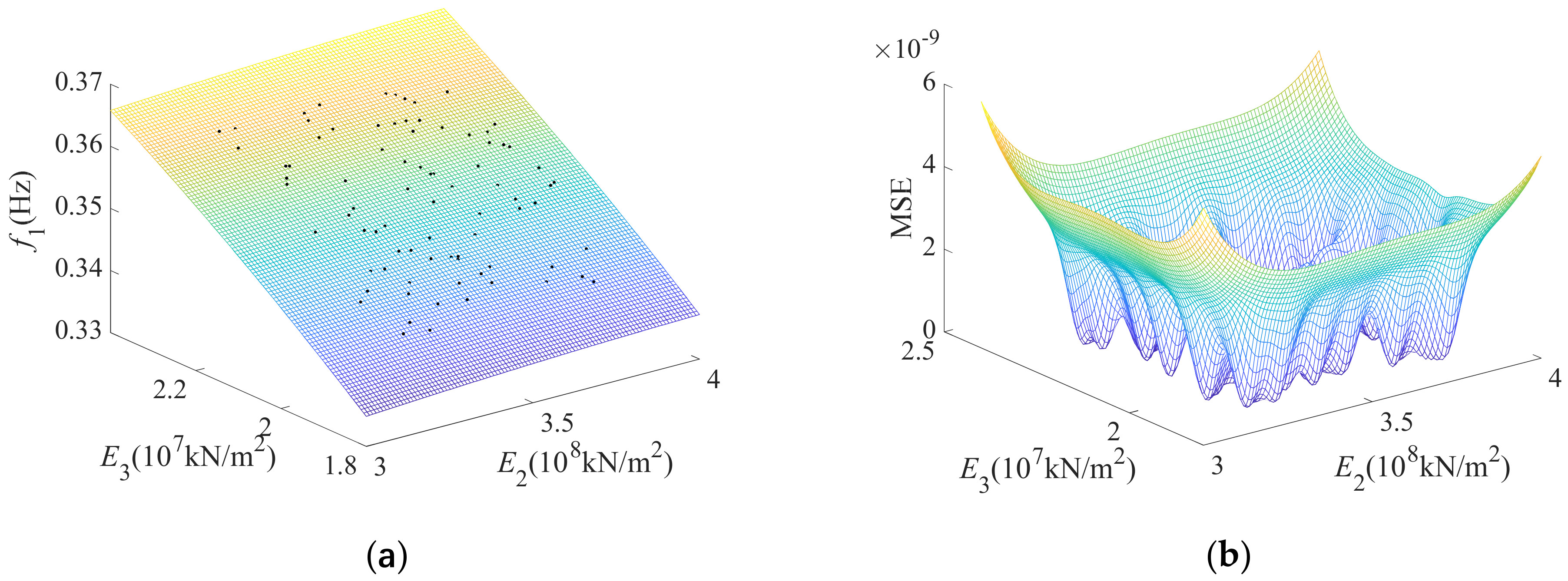
Figure 6 plots the kriging response surface model and the corresponding mean square error (MSE) for the first-order frequency versus the updating parameters E₁ and E₂. The surface represents the kriging model response surface, the scattered points represent the sample points, and the sample points are located on the curved surface. It can be seen from the MSE surface that the maximum error is less than 4 × 10⁻⁷, indicating that the kriging model has high accuracy and can replace the FE model in predicting the structural response.

The first six frequency residuals of the truss are used to construct the objective function, and the three standard optimization algorithms and the corresponding improved algorithms are used to find the global minimum of the objective function. The objective function is expressed by:

$$\min fit(x)=\min {{\displaystyle \sum _{i=1}^6{\omega }_i\left(\frac{f_{ai}-f_{ei}}{f_{ei}}\right)}}^2,$$

(18)

where fit(x) represents the objective function; $x$ represents the updating parameter; ${\omega }_i$ represent the weight factor, which is set to 1 [6]; $f_{ai}$ is the i-th order frequency value calculated by the kriging response surface model; and $f_{ei}$ is the i-th order frequency value calculated by the FE model.

Regarding the algorithm parameters, in order to ensure the comparability between different algorithms, the population size of each algorithm is 50, and the maximum number of iterations is 100. For PSO, the learning factors $c_1$ and $c_2$ are 1.5 and 0.5, respectively, and the inertia constant is 0.726. For GSA, the universal gravitation coefficient $G_0$ is 10, and the descent coefficient $\alpha$ is 20. The attenuation parameter of the SA algorithm is 0.95, the initial temperature is set at 50, and the final temperature is set to 0.

Table 2. The change of updating parameters in model updating.

Parameters		E1 (100 GPa)	E2 (100 GPa)	E3 (100 GPa)	Relative Error (%)
Damaged Model		0.7	0.7	1.3	-
Initial model		1	1	1	42.86	42.86	−23.08
Updated model	IGSA	0.705	0.714	1.282	0.71	2.00	−1.38
	GSA	0.738	0.682	1.280	5.43	−2.57	−1.54
	IPSO	0.727	0.740	1.320	3.86	5.71	1.54
	PSO	0.740	0.771	1.315	5.71	10.14	1.15
	ISA	0.700	0.695	1.311	0.00	−0.71	0.85
	SA	0.703	0.673	1.342	0.43	−3.86	3.23

shows the change in updating parameters in different algorithms. The relative error means the discrepancy of the updating parameters between the updated model and the predetermined damage value. The smaller the relative error, the higher the updated model’s accuracy. It can be seen from Table 2 that relative errors obtained with improved algorithms are all smaller than that obtained with standard algorithms. For example, the relative errors of E₁ obtained from IGSA and GSA are 0.74% and 5.49%. These data indicate that the improved algorithms are better than standard algorithms in model updating. Nevertheless, the updating results of each algorithm still need further discussion.

Table 3. The comparison of the first six frequencies obtained from the initial FE model and updated FE model.

Frequency		f1 (Hz)	f2 (Hz)	f3 (Hz)	f4 (Hz)	f5 (Hz)	f6 (Hz)	Relative Error (%)
Damage Model		7.50	15.72	19.57	23.67	31.42	33.68	-
Initial model		7.63	16.65	20.18	25.16	32.54	34.32	1.73	5.92	3.12	6.29	3.56	1.90
Updated model	IGSA	7.50	15.71	19.61	23.71	31.45	33.67	0.00	−0.06	0.20	0.17	0.10	−0.03
	GSA	7.50	15.72	19.61	23.71	31.46	33.68	0.00	0.00	0.20	0.17	0.13	0.00
	IPSO	7.54	15.87	19.69	23.88	31.59	33.91	0.53	0.95	0.61	0.89	0.54	0.68
	PSO	7.55	15.96	19.76	24.01	31.70	34.00	0.67	1.53	0.97	1.44	0.89	0.95
	ISA	7.50	15.7	19.57	23.65	31.41	33.70	0.00	−0.13	0.00	−0.08	−0.03	0.06
	SA	7.50	15.71	19.54	23.61	31.37	33.74	0.00	−0.06	−0.15	−0.25	−0.16	0.18

compares the first six frequencies of the truss structure obtained from the initial FE model and the updated FE model. The frequencies of the damage model are also listed for comparison. It can be seen that the maximum relative errors of the six frequencies obtained from the initial FE model and updated FE model are 6.29% and 1.44%, respectively, indicating that the accuracy of the updated FE model has been greatly improved. All relative errors of the updated FE model, obtained with improved algorithms, are smaller than 1%. The improved algorithms obtained a more accurate updated FE model than the standard algorithms.

Table 4. The mean and standard deviation of the objective function.

Algorithm	IGSA	GSA	IPSO	PSO	ISA	SA
Mean	2.56 × 10−4	5.20 × 10−4	1.91 × 10−4	8.16 × 10−4	9.64 × 10−1	9.72 × 10−1
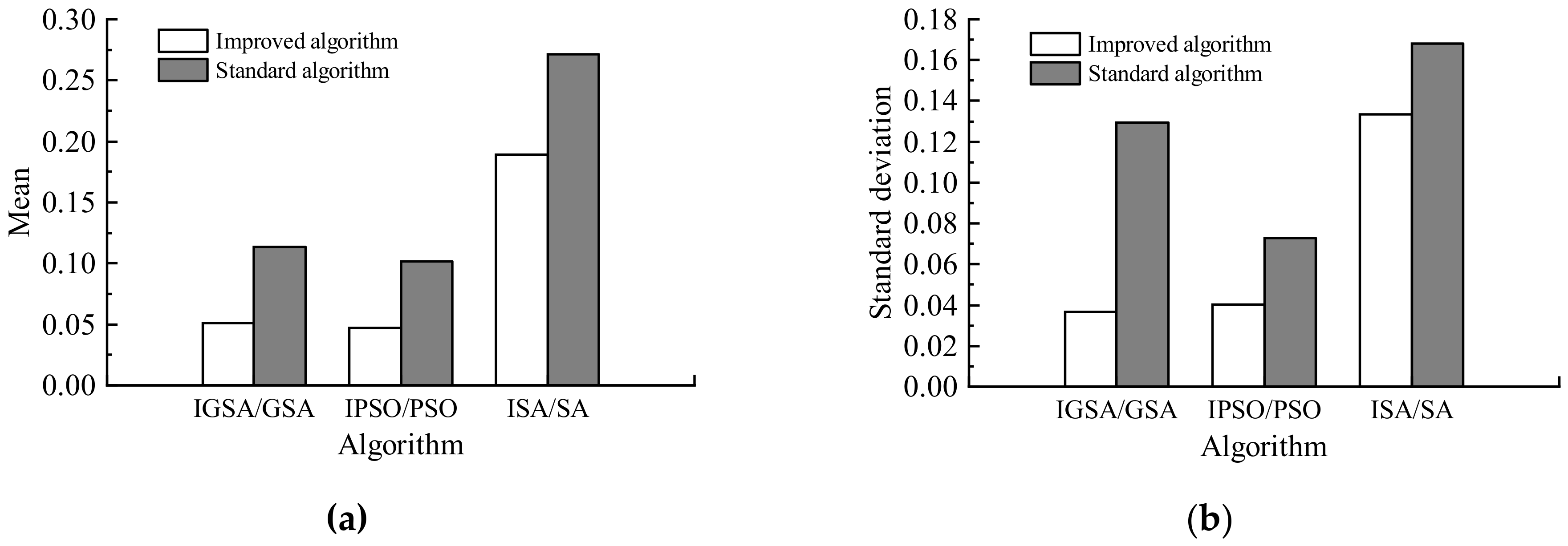
Standard deviation	7.61 × 10−3	1.65 × 10−2	1.74 × 10−3	2.00 × 10−2	1.04 × 10−1	1.36 × 10−1

summarizes the statistical results of the updating results obtained from 100 independent runs of each algorithm. It can be seen that all improved algorithms have a smaller mean and standard deviation value compared with the standard algorithms. This result indicates that the improved algorithm has higher searching accuracy and stability than standard algorithms.

5. Case Study: FE Model Updating of a Cable-Stayed Bridge

5.1. Bridge Description

The Yongjiang Railway Bridge is located in Ningbo, China. The main bridge of the Yongjiang Bridge is a double-pylon double cable plane cable-stayed bridge with a hybrid girder composed of a steel box girder and a concrete box girder. The span layout of the main bridge is 53 + 50 + 50 + 66 + 468 + 66 + 50 + 50 + 53 m, in which the 400.9 m girder section of the middle span is a steel box girder, and the stiffness transition section is 5.0 m long. The length of the steel-concrete joint section is 7.35 m, and the rest of the beam sections are pre-stressed concrete box girders. The steel box girder is enclosed by a top plate, bottom plate, inclined bottom plate, middle longitudinal web, side longitudinal web, and side plate. The concrete box girder adopts a single box, three rooms, and an equal height section. The height of the two pylons is 141.5 m. The width of the bridge deck is 21 m, on top of which are laid two railway lines in opposite directions. Figure 7 shows the layout of the bridge.

The bridge’s initial FE model (Figure 8) was established based on Midas Civil 2012. The beam element simulates the concrete/steel/reinforced concrete structural members such as the beam body, bridge tower, pier, and pile cap. The stay-cables were modeled using a truss element. Vertical supports were provided at P1 #~P4 # and P7 #~P10 # piers for side span longitudinal beams on both banks. An elastic connection was adopted between the main beam and the cross-tie beam between the bridge towers. The bridge structure is a semi-floating system. The pier and foundation were consolidated. In total, 999 beam elements and 200 truss elements were used in the initial FE model.

5.2. In Situ Tests and Experimental Results

The in situ tests of the Yongjiang Bridge included two parts: static load tests and dynamic load tests. Figure 9 shows the loading train and the data acquisition system employed in the in situ testing. In the static load tests, the displacements of the main girder were recorded under six load cases, namely test cases A~F. The position of loading trains in each load case was determined using the influence line method based on the most unfavorable loading principle. Figure 7b shows the location of the loading train of each load case and the displacement measuring points’ locations. For the number of loading trains for each load case, cases A and D include one locomotive, and twelve freights. Load cases B and C include one locomotive and four freights, and load cases E and F include one locomotive and 20 freights. Figure 10 shows the axial load distribution of the loading trains used in the static load tests. The loading trains were disassembled according to each load case to meet the most unfavorable loading condition. The load efficiency coefficients of each load case were between 0.75 and 0.88.

In the dynamic tests, the accelerations of the bridge deck were recorded under ambient excitation. In total, the accelerations at 65 measuring points were recorded. The sampling frequency and sampling time for each setup were 200 Hz and 15 min, respectively. The bridge’s natural frequencies and mode shapes were identified utilizing stochastic subspace identification.

Table 5. Calculated value and test value of displacement of each measuring point under each load case.

Test Cases	Test Section	Experimental Value (mm)			Initial FE Model (mm)	Relative Error (%)
		Upstream	Downstream	Mean
A	1	414.00	412.60	413.30	486.21	17.64
	2	394.60	386.60	390.60	410.60	5.12
B	1	211.00	213.00	212.00	237.14	11.86
	2	240.00	236.30	238.15	258.12	8.39
C	3	102.00	110.00	106.00	125.73	18.61
	4	139.00	139.60	139.30	161.31	15.80
D	2	263.00	264.30	263.65	304.01	15.31
	3	353.00	350.40	351.70	442.41	25.79
E	2	313.00	311.80	312.40	370.15	18.49
	3	386.00	386.80	386.40	489.42	26.66
F	1	435.00	434.50	434.75	569.27	30.94
	2	555.00	542.40	548.70	624.84	13.88

summarizes the experimental measured displacement values and the corresponding predicted values by the initial FE model. Each test section has two displacement measuring points; therefore, the experimental measured values include the upstream and downstream value. The mean value of the upstream and downstream displacement value were included in the model updating. The displacement’s maximum relative error reaches up to 30.94%, indicating the initial FE model should be updated.

Figure 11 shows the comparison of the first two order mode shapes between their experimental measured values and calculated values from the initial FE model. It can be seen that the calculated vibration modes are in good agreement with the measured ones.

Table 6. Calculated value and test value of frequency.

Vibration Mode	Experimental Value (Hz)	Initial FE Model (Hz)	MAC	Relative Error (%)
1	0.390	0.347	0.936	−11.03
2	0.490	0.456	0.947	−6.94

summarizes the first two modes calculated and the experimental frequency values. The experimental values are slightly higher than the calculated ones, which implies that the stiffness of the initial model is smaller than the actual structure. It can be seen that the modal assurance criterion (MAC) [40] values of the measured and calculated vibration modes are 0.936 and 0.947, respectively, which are larger than 0.9. This result indicates that the experimentally identified, first two frequencies can be further used to update the initial FE model.

5.3. Selection of Updating Parameters

The selection of the updating parameters was carried out by considering the following facts. On the one hand, the prefabricated steel segments in the primary structure give comparatively small errors in the cross-section profile. On the other hand, the initial FE model for the bridge was mainly simplified in local stiffening ribs, which affects the stiffness and mass distribution of the whole structure. Therefore, the material properties, including elastic modulus and density, were selected as the updating parameters for sensitivity analysis. The selected design parameters for sensitivity analysis include the elastic modulus and mass density of the concrete box girder (E₁, D₁), steel box girder (E₂, D₂), bridge pylon (E₃, D₃), pier (E₄, D₄), stay cable (E₅, D₅), and secondary tension of three stay cables (F₁, F₂, F₃). Figure 12 shows the results of the sensitivity analysis. In Figure 12, the MAC1 and MAC2 are the MAC values of the first and second mode shapes, respectively. The f₁ to f₂ are the first two natural frequencies, respectively.

For sensitivity analysis, this study selected the elastic modulus of steel box girder E₂, the density of steel box girder D₂, the elastic modulus of bridge pylon E₃, the density of bridge pylon D₃, elastic modulus of stay cable E₅, and the density of stay cable D₅ as the updating parameters, and their initial values were 2.1 × 10⁸ kN/m², 78.5 kN/m³, 3.55 × 10⁷ kN/m², 25 kN/m³, 2.1 × 10⁸ kN/m², 84.5 kN/m³, respectively.

5.4. Kriging Model Construction

The selected six parameters were sampled 81 times in their design space by using latin hypercube sampling to establish the kriging model. The sampling range of the parameters was set at 0.7~1.3 times their initial value to ensure the physical meaning of each updating parameter [41]. Then 81 groups of samples were input into the initial FE model to calculate the displacement response and frequency response under the corresponding load. The kriging model was constructed with sampling points as input, node displacement, and modal frequency response as output.

Figure 13a shows the relationship between the first frequency and E2 and E3. The surface in Figure 13a represents the kriging predicted value, and the dots are analytical values obtained from the initial FE model. Since the frequency kriging model includes six updating parameters, the other four updating parameters (D₂, D₃, E₅, and D₅) are set as initial values when calculating the analytical values. Figure 13b shows the kriging model’s mean square error (MSE). The maximum error is smaller than 6 × 10⁻⁹, indicating that the kriging predicted value has very high accuracy and can replace the FE model when calculating the response values.

5.5. Objective Function

In the model updating of Yongjiang Bridge, the relative error between the response value obtained from the kriging response surface and the measured value is used as the objective function, and the objective function is expressed by:

$$\min fit(x)=\min ({{\displaystyle \sum _{i=1}^{12}{\omega }_i\left(\frac{d_{ai}-d_{ei}}{d_{ei}}\right)}}^2+{{\displaystyle \sum _{j=1}^2{\omega }_j\left(\frac{f_{aj}-f_{ej}}{f_{ej}}\right)}}^2).$$

(19)

where fit(x) represents the objective function values; $x$ represents the updating parameter; ${\omega }_i$ and ${\omega }_{\mathrm{j}}$ represent the weight factors; $d_{ai}$ and $f_{aj}$ are the i-th displacement value and the j-th order frequency value calculated by the kriging response surface model, respectively; and $d_{ei}$ and $f_{ej}$ are the i-th displacement value and the j-th order frequency value measured by Yongjiang Bridge, respectively.

5.6. Discussion on the Updating Results

The standard algorithms and their improved versions were employed to find the optimal solution for the objective function. The algorithms’ parameters were the same as that used in the numerical simulation of the truss structure. The weighting factors of frequencies and displacements were all set as 1.

Table 7. Comparison of the design parameters between initial values and updated values.

Parameters	Initial Value	Updated Value						Updating Rate (%)
		IGSA	GSA	IPSO	PSO	ISA	SA	IGSA	GSA	IPSO	PSO	ISA	SA
E2	3.55	4.23	4.35	4.17	3.83	3.20	4.60	19.15	22.54	17.46	7.89	−9.86	29.58
D2	2.50	2.78	2.65	2.72	2.59	2.72	2.60	11.20	6.00	8.80	3.60	8.80	4.00
E3	2.10	2.42	2.42	2.39	2.29	2.29	2.31	15.24	15.24	13.81	9.05	9.05	10.00
D3	7.85	7.25	8.14	7.66	7.07	7.07	7.19	−7.64	3.69	−2.42	−9.94	−9.94	−8.41
E5	2.00	2.52	2.46	2.47	2.50	2.48	2.55	26.00	23.00	23.50	25.00	24.00	27.50
D5	8.45	9.89	9.43	9.40	8.56	7.92	9.75	17.04	11.60	11.24	1.30	−6.27	15.38

shows the comparison of the updating parameters between their initial values and updated values obtained from each algorithm. The updated values obtained from each standard algorithm and its improved version generally show the same change trend; however, there also exist exceptions. For example, all six parameters have the same change trend in PSO and IPSO, while the change trends of E₁ obtained from SA and ISA are totally different. Except for D₂, an overall increase in the rest of the parameters is apparent. A similar updating rate of elastic modulus for a cable-stayed bridge can be found in reference [42]. This increase indicates that the stiffness and mass distribution of the initial FE model is underestimated. The reason for this could be attributed to the simplifications of the local stiffening ribs, diaphragms, and other local members in the initial FE model. The parameters’ updated values obtained from different algorithms are different, indicating that each algorithm and its improved version converged to a different solution in the design space. It should be mentioned that the changes in the updating parameters only represent the change in the overall stiffness and mass between the FE model and the physical structure. Therefore, the updating parameters can be viewed as equivalent elastic modulus and equivalent density. Nevertheless, the rationality of the updated FE model still needs to be evaluated by analyzing the prediction accuracy.

Figure 14 compares the displacement values obtained from the experiment, initial FE model, and updated FE models.

Table 8. Comparison of the displacement relative errors between the initial FE model and updated FE models.

Load Case		A		B		C		D		E		F
Test Section		1	2	1	2	3	4	2	3	2	3	1	2
Initial error (%)		17.64	5.12	11.86	8.39	18.61	15.80	15.31	25.79	18.49	26.66	30.94	13.88
Relative error (%)	IGSA	0.34	−9.51	−4.08	−6.36	−0.02	−2.76	−1.01	6.81	1.35	7.64	11.33	−2.00
	GSA	0.01	−9.96	−4.48	−6.84	−0.14	−2.66	−1.49	7.10	1.85	7.94	11.75	−2.48
	IPSO	0.29	−9.73	−4.07	−6.36	−0.36	−2.04	−1.41	7.16	1.62	7.94	11.35	−2.29
	PSO	0.36	−9.77	−4.19	−6.67	0.27	−2.17	−1.25	7.22	1.62	8.04	11.66	−2.28
	ISA	0.40	−9.32	−3.45	−5.46	0.50	−1.28	−1.35	7.42	1.62	7.99	11.38	−1.85
	SA	0.58	−9.99	−4.27	−7.05	−1.00	−2.81	−1.37	7.28	1.69	8.23	11.64	−2.56

summarizes the displacement relative errors of the initial FE model and updated FE models. Compared with the initial FE model, it is obvious that the updated model obtained from each algorithm provides higher prediction accuracy. The displacement relative errors have a significant decrease after model updating except for the displacement at Test section 2 for load case A. Nevertheless, the displacement relative errors of the updated model are generally controlled at around 10%, which is an acceptable accuracy level from an engineering judgment perspective. Compared with the standard algorithm, the improved algorithms achieved a slightly higher accuracy. For example, the displacement relative errors of Test section 3 in load case D obtained from IGSA and GSA are 6.81% and 7.10%, respectively, indicating that the prediction accuracy of the updated model obtained from IGSA is higher than GSA. A similar situation can be found in the other two algorithms. These results indicate that the improved algorithm performs better than standard algorithms.

Table 9. Comparisons of the frequencies obtained from experiment and the initial FE model and updated FE models.

Frequency		f1 (Hz)	f2 (Hz)	Relative Error (%)
Experimental Value		0.390	0.490
Initial FE model		0.347	0.456	−11.03	−6.94
Updating models	IGSA	0.374	0.479	−4.10	−2.24
	GSA	0.366	0.474	−6.15	−3.27
	IPSO	0.371	0.485	−4.87	−1.02
	PSO	0.369	0.476	−5.38	−2.86
	ISA	0.370	0.486	−5.13	−0.82
	SA	0.370	0.479	−5.13	−2.24

shows comparisons between the frequencies obtained from the experiment and the initial FE model and updated FE models. It can be seen that the updated models obtained from each algorithm provide higher frequency prediction accuracy. After model updating, the frequency relative error is reduced to a level of 5%. Compared with the standard algorithms, the improved algorithms provide even smaller relative errors. For example, the relative error of f₁ obtained from GSA is −6.15%, while that obtained from IGSA is −4.10%. These results indicate that the improved algorithms perform better than standard algorithms in predicting frequency.

Figure 15 shows the statistical results of the updating results obtained from 100 independent runs of each algorithm. In Figure 15, the mean values of the objective function obtained from IGSA and GSA are 5.14 × 10⁻² and 1.14 × 10⁻¹, respectively. The corresponding standard deviations are 3.65 × 10⁻² and 1.29 × 10⁻¹, respectively. The mean value and standard deviation of IGSA are smaller than those of GSA. The same situation is observed for the other two algorithms. These results indicate that the improved algorithms have higher accuracy and stability.

6. Conclusions

This study proposes an improvement strategy for metaheuristic algorithms, improving the algorithm’s performance in model updating. The improvement strategy introduces random crossover and mutation operations into the workings of standard metaheuristic algorithms to improve the searching accuracy at later stages. Three widely used metaheuristic algorithms, namely PSO, GSA, and SA, were employed to test the effectiveness of the improvement strategy. Based on the numerical investigations on the benchmark functions and a spatial truss structure, and the experimental study of the model updating of a cable-stayed railway bridge, the following conclusions can be drawn:

(1)

The proposed improvement strategy can effectively improve the accuracy and the global convergence of standard metaheuristic algorithms. The random crossover and mutation operations are mainly introduced during later-stage searching and aim to improve the algorithm’s accuracy;

(2)

The numerical investigation of the two benchmark functions showed that the improved algorithms had better global convergence and stability than the standard algorithms. The updated truss model with the improved algorithms showed higher prediction accuracy than the standard algorithm;

(3)

The discrepancies between the calculated and experimental values of displacement and frequency of the cable-stayed bridge were much smaller after model updating. The updated models with the improved algorithm had smaller relative errors than those obtained with the standard algorithms. In the IGSA algorithm, for example, the relative error in displacement was significantly reduced, with the maximum relative error reduced from 30.94% to 11.33% and the relative error in first-order frequency reduced from 11.03% to 4.21%, indicating that the updated model can better represent the actual structure.

References

1. Hao, S. I-35W bridge collapse. J. Bridge Eng. 2010, 15, 608–614. [Google Scholar] [CrossRef]
2. Keary, H.; Sara, J. Fault tree analysis of Schoharie creek bridge collapse. J. Perform. Constr. Facil. 2007, 21, 320–326. [Google Scholar]
3. Joel, M.; Diogo, R.; Carlos, S.; Rui, C. Model updating of a dynamic model of a composite steel-concrete railway viaduct based on experimental tests. Eng. Struct. 2018, 164, 40–52. [Google Scholar]
4. Yang, Y.; Chen, Y. A new direct method for updating structural models based on measured modal data. Eng. Struct. 2009, 31, 32–42. [Google Scholar] [CrossRef]
5. Zhou, L.; Wang, L.; Chen, L.; Ou, J. Structural finite element model updating by using response surfaces and radial basis functions. Adv. Struct. Eng. 2016, 19, 1446–1462. [Google Scholar] [CrossRef]
6. Ren, W.; Chen, H. Finite element model updating in structural dynamics by using the response surface method. Eng. Struct. 2010, 32, 2455–2465. [Google Scholar] [CrossRef]
7. Simoen, E.; De, R.G.; Lombaert, G. Dealing with uncertainty in model updating for damage assessment: A review. Mech. Syst. Signal Process. 2015, 56, 123–149. [Google Scholar] [CrossRef] [Green Version]
8. Klein, S.; Pluim, J.P.W.; Staring, M. Adaptive stochastic gradient descent optimisation for image registration. Int. J. Comput. Vis. 2009, 81, 227–239. [Google Scholar] [CrossRef] [Green Version]
9. Cuadros Angela, P.; Arce Gonzalo, R. Coded aperture optimization in compressive X-ray tomography: A gradient descent approach. Opt. Express 2017, 25, 23833–23849. [Google Scholar] [CrossRef]
10. Hurtado, J.E.; Robinett, R.D. Convergence of Newton’s method via Lyapunov analysis. J. Guid. Control. Dynam. 2005, 28, 363–365. [Google Scholar] [CrossRef]
11. Jiang, J.; Shui, P. Design of 2D oversampled linear phase DFT modulated filter banks via modified Newton’s method. Signal Process. 2012, 92, 1411–1421. [Google Scholar] [CrossRef]
12. Nickabadi, A.; Ebadzadeh, M.M.; Safabakhsh, R. A novel particle swarm optimization algorithm with adaptive inertia weight. Appl. Soft Comput. 2011, 11, 3658–3670. [Google Scholar] [CrossRef]
13. Liu, Y.; Huang, S.; Huang, J.; Liang, W. A Particle Swarm Optimization-Based Maximum Power Point Tracking Algorithm for PV Systems Operating Under Partially Shaded Conditions. IEEE Trans. Energy Convers. 2012, 27, 1027–1035. [Google Scholar] [CrossRef]
14. Karaboga, D.; Gorkemli, B.; Ozturk, C.; Karaboga, N. A comprehensive survey: Artificial bee colony (ABC) algorithm and applications. Artif. Intell. Rev. 2014, 42, 21–57. [Google Scholar] [CrossRef]
15. Alatas, B. Chaotic bee colony algorithms for global numerical optimization. Expert Syst. Appl. 2010, 37, 5682–5687. [Google Scholar] [CrossRef]
16. Gao, Y.; Guan, H.; Qi, Z.; Hou, Y.; Liu, L. A multi-objective ant colony system algorithm for virtual machine placement in cloud computing. J. Comput. Syst. Sci. 2013, 79, 1230–1243. [Google Scholar] [CrossRef]
17. Tabakhi, S.; Moradi, P.; Akhlaghian, F. An unsupervised feature selection algorithm based on ant colony optimization. Eng. Appl. Artif. Intell. 2014, 32, 112–123. [Google Scholar] [CrossRef]
18. Rashedi, E.; Nezamabadi-Pour, H.; Saryazdi, S. BGSA: Binary gravitational search algorithm. Nat. Comput. 2010, 9, 727–745. [Google Scholar] [CrossRef]
19. Rashedi, E.; Nezamabadi-Pour, H.; Saryazdi, S. Filter modeling using gravitational search algorithm. Eng. Appl. Artif. Intell. 2011, 24, 117–122. [Google Scholar] [CrossRef]
20. Huang, M.; Gül, M.; Zhu, H. Vibration-Based Structural Damage Identification under Varying Temperature Effects. J. Aerosp. Eng. 2018, 31, 04018014. [Google Scholar] [CrossRef]
21. Huang, M.; Lei, Y.; Li, X.; Gu, J. Damage Identification of Bridge Structures Considering Temperature Variations-Based SVM and MFO. J. Aerosp. Eng. 2021, 34, 04020113. [Google Scholar] [CrossRef]
22. Boussaid, I.; Lepagnot, J.; Siarry, P. A survey on optimization metaheuristics. Inform. Sci. 2013, 237, 82–117. [Google Scholar] [CrossRef]
23. Blum, C.; Roli, A. Metaheuristics in combinatorial optimization: Overview and conceptual comparison. ACM Comput. Surv. 2003, 35, 268–308. [Google Scholar] [CrossRef]
24. Ding, Z.; Fu, K.; Deng, W.; Li, J.; Lu, Z. A modified Artificial Bee Colony algorithm for structural damage identification under varying temperature based on a novel objective function. Appl. Math. Model. 2020, 88, 122–141. [Google Scholar] [CrossRef]
25. Yang, F. Autonomous vehicle routing problem solution based on artificial potential field with parallel ant colony optimization (ACO) algorithm. Pattern Recognit. Lett. 2018, 116, 195–199. [Google Scholar]
26. Jiang, Y.; Hu, T.; Huang, C. An improved particle swarm optimization algorithm. Appl. Math. Comput. 2007, 193, 231–239. [Google Scholar] [CrossRef]
27. Marzband, M.; Ghadimi, M.; Sumper, A.; José Luis Domínguez-García, c. Experimental validation of a real-time energy management system using multi-period gravitational search algorithm for microgrids in islanded mode. Appl. Energy 2014, 128, 164–174. [Google Scholar] [CrossRef] [Green Version]
28. Wang, F.; Wang, J.; Chen, X. Evacuation entropy path planning model based on hybrid ant colony-artificial fish swarm algorithms. In Proceedings of the 2nd International Conference on Advanced Electronic Materials: Computers and Materials Engineering, Changsha, China, 3 April 2019. [Google Scholar]
29. Hu, H.; Cui, X.; Bai, Y. Two kinds of classifications based on improved gravitational search algorithm and particle swarm optimization algorithm. Adv. Math. Phys. 2017, 2017, 2131862. [Google Scholar] [CrossRef] [Green Version]
30. Huang, M.; Cheng, X.; Lei, Y. Structural damage identification based on substructure method and improved whale optimization algorithm. J. Civ. Struct. Health 2021, 11, 351–380. [Google Scholar] [CrossRef]
31. Luo, J.; Huang, M.; Xiang, C.; Lei, Y. Bayesian damage identification based on autoregressive model and MH-PSO hybrid MCMC sampling method. J. Civ. Struct. Health 2022, 12, 361–390. [Google Scholar] [CrossRef]
32. Echard, B.; Gayton, N.; Lemaire, M. AK-MCS: An active learning reliability method combining Kriging and Monte Carlo Simulation. Struct. Saf. 2011, 33, 145–154. [Google Scholar] [CrossRef]
33. Yang, X.; Guo, X.; Ouyang, H.; Li, D. A Kriging Model Based Finite Element Model Updating Method for Damage Detection. Appl. Sci. 2017, 7, 1039. [Google Scholar] [CrossRef] [Green Version]
34. Wang, J.; Wang, C.; Zhao, J. Frequency response function-based model updating using Kriging model. Mech. Syst. Signal Process. 2017, 87, 218–228. [Google Scholar] [CrossRef]
35. Zhang, J.; Au, F.T.K.; Yang, D. Finite element model updating of long-span cable-stayed bridge by Kriging surrogate model. Struct. Eng. Mech. 2020, 74, 157–173. [Google Scholar]
36. Mao, J.; Wang, H.; Li, J. Bayesian Finite Element Model Updating of a Long-Span Suspension Bridge Utilizing Hybrid Monte Carlo Simulation and Kriging Predictor. KSCE J. Civ. Eng. 2020, 24, 569–579. [Google Scholar] [CrossRef]
37. Deb, K.; Pratap, A.; Agarwal, S.; Meyarivan, T. A fastand elitist multiobjective genetic algorithm: NSGA-II. IEEE Trans. Evol. Comput. 2002, 6, 182–197. [Google Scholar] [CrossRef] [Green Version]
38. Li, H.; Zhang, Q. Multiobjective optimization problems with complicated pareto sets, MOEA/D and NSGA-II. IEEE Trans. Evol. Comput. 2009, 13, 284–302. [Google Scholar] [CrossRef]
39. Kao, Y.; Zahara, E. A hybrid genetic algorithm and particle swarm optimization for multimodal functions. Appl. Soft. Comput. 2008, 8, 849–857. [Google Scholar] [CrossRef]
40. Liu, W.; Gao, W.; Sun, Y.; Xu, M. Optimal Sensor Placement for Spatial Lattice Structure Based on Genetic Algorithms. J. Sound Vib. 2008, 317, 175–189. [Google Scholar] [CrossRef]
41. Zhong, J.; Gou, H.; Zhao, H.; Zhao, T.; Wang, X. Comparison of several model updating methods based on full-scale model test of track beam. Structures 2022, 35, 46–54. [Google Scholar] [CrossRef]
42. Wang, F.; Xu, Y.; Sun, B.; Zhu, Q. Updating Multiscale Model of a Long-Span Cable-Stayed Bridge. J. Bridge Eng. 2018, 23, 04017148. [Google Scholar] [CrossRef]
Figure 1. Flow chart of the improved algorithm.
Buildings 12 00958 g001
Figure 2. Image of the benchmark functions: (a) Ackley’s path function; and (b) the sum of different power function.
Buildings 12 00958 g002
Figure 3. The convergence curves of each algorithm for the two functions: (a) f1; and (b) f2.
Buildings 12 00958 g003
Figure 4. The simply supported truss structure. (Unit: cm).
Buildings 12 00958 g004
Figure 5. The first six mode shapes of the truss: (a) first order mode; (b) the second mode; (c) the third mode; (d) the fourth mode; (e) the fifth mode; and (f) the sixth mode.
Buildings 12 00958 g005
Figure 6. The first-order frequency kriging model and the corresponding MSE: (a) kriging model; and (b) MSE.
Buildings 12 00958 g006
Figure 7. The Yongjiang Bridge: (a) overview; (b) the elevation layout; (c) the section layout of the steel box girder; and (d) the section layout of the concrete box girder. (Unit: cm).
Buildings 12 00958 g007
Figure 8. The initial FE model of the Yongjiang Bridge.
Buildings 12 00958 g008
Figure 9. Photos of in situ test: (a) the loading train and (b) the instrumentation and data acquisition system.
Buildings 12 00958 g009
Figure 10. The Wheelbase Distribution of the Locomotive/Freight Car. (Unit: m).
Buildings 12 00958 g010
Figure 11. Measured vibration mode and calculated vibration mode MAC: (a) first order mode and (b) the second mode.
Buildings 12 00958 g011
Figure 12. Updating parameter sensitivity.
Buildings 12 00958 g012
Figure 13. Kriging model: (a) first order frequency response surface and (b) MSE error of the first-order frequency.
Buildings 12 00958 g013
Figure 14. The comparison of the displacement values obtained from experiment (EXP), initial FE model and updated FE models: (a) load case A and B; (b) load case C and D; and (c) load case E and F.
Buildings 12 00958 g014aBuildings 12 00958 g014b
Figure 15. The mean and standard deviation of the objective function. (a) Mean; (b) Standard deviation.
Buildings 12 00958 g015