
Hybrid Models for Indoor Temperature Prediction Using Long Short Term Memory Networks—Case Study Energy Center


Abstract
:1. Introduction
2. Materials and Methods
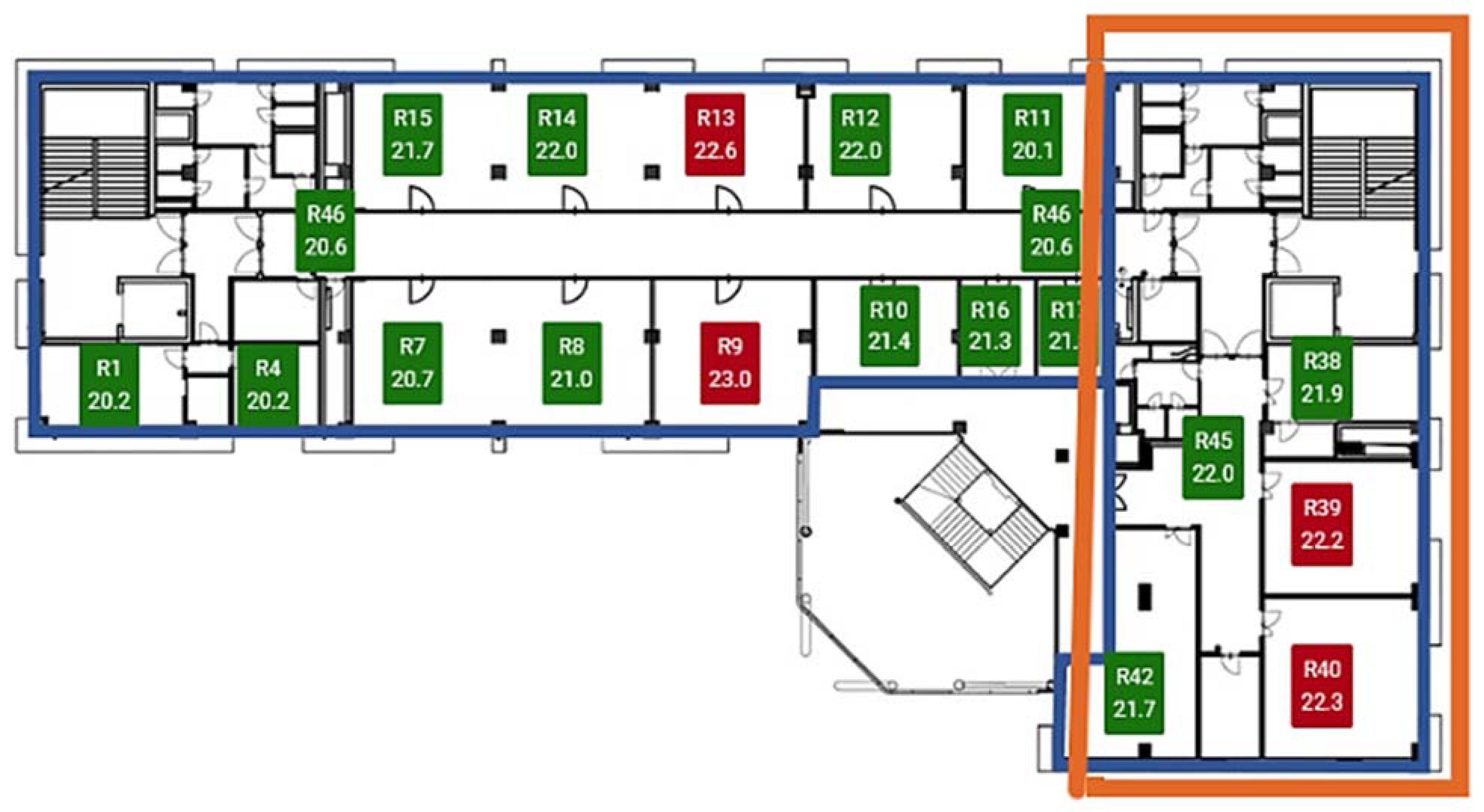
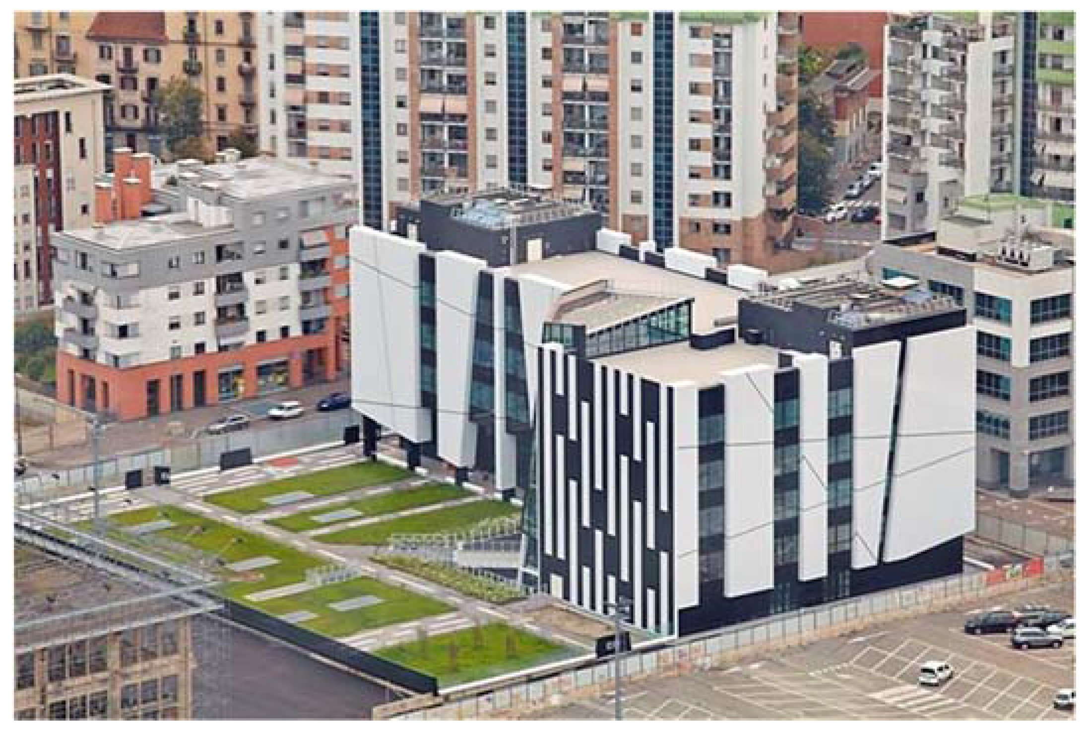
2.1. The Target Building
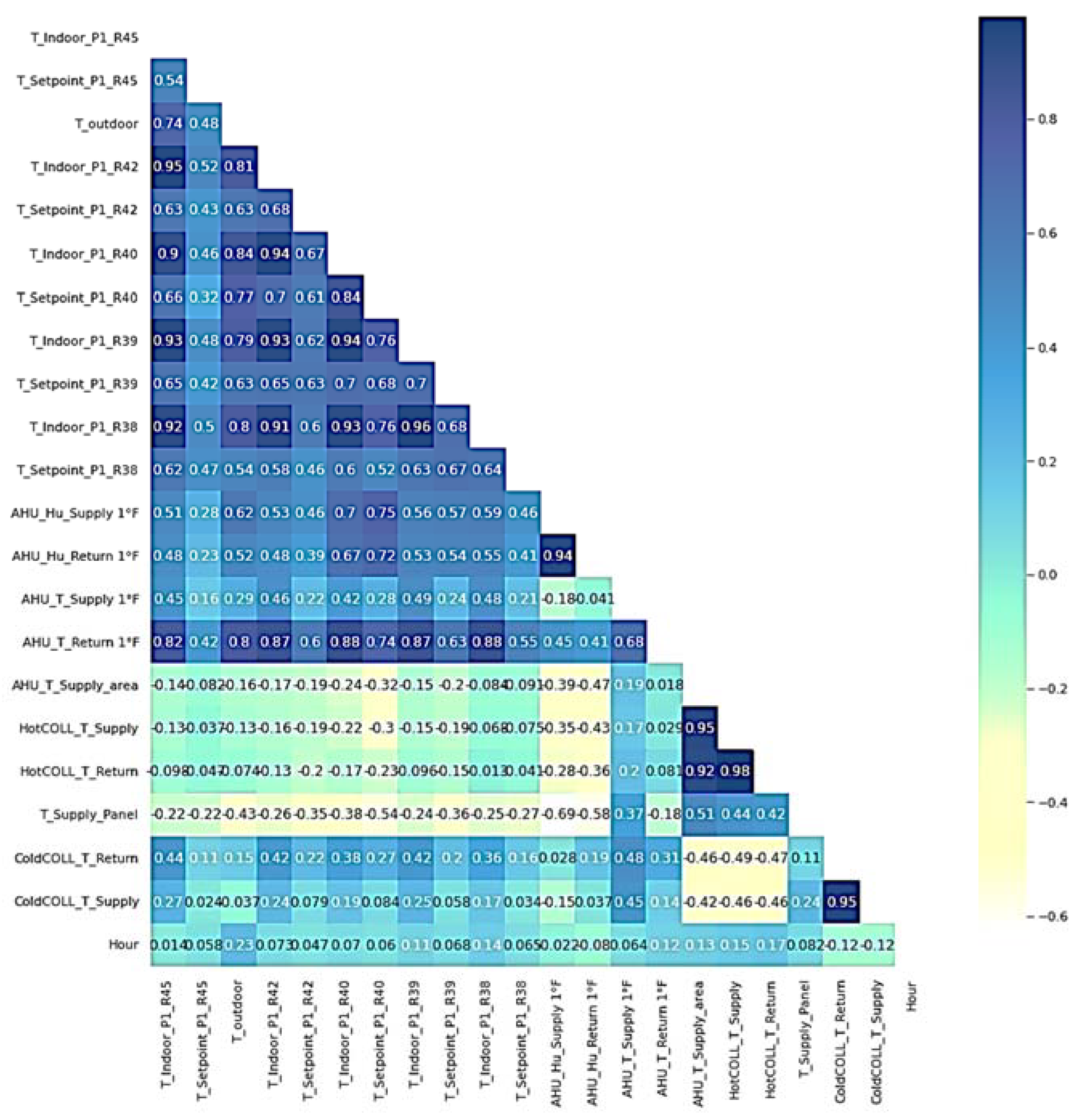
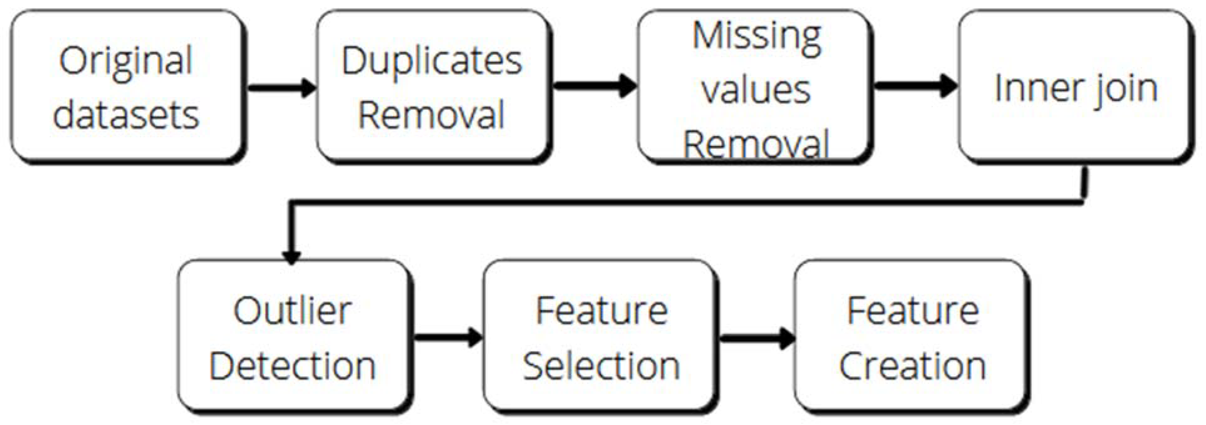
2.2. The Dataset
2.3. Possible Approaches
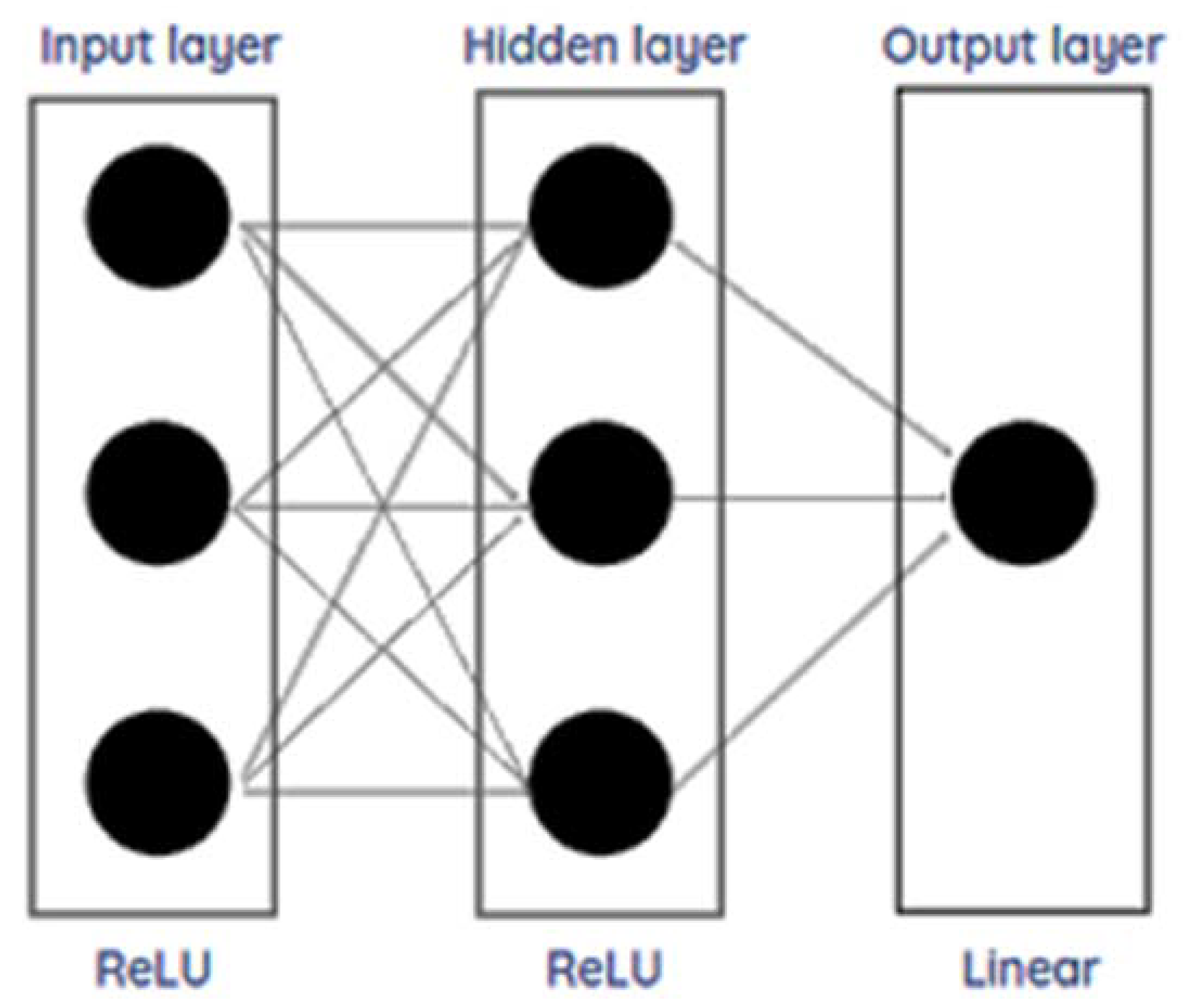
2.4. The Model
2.5. The Dataset Split
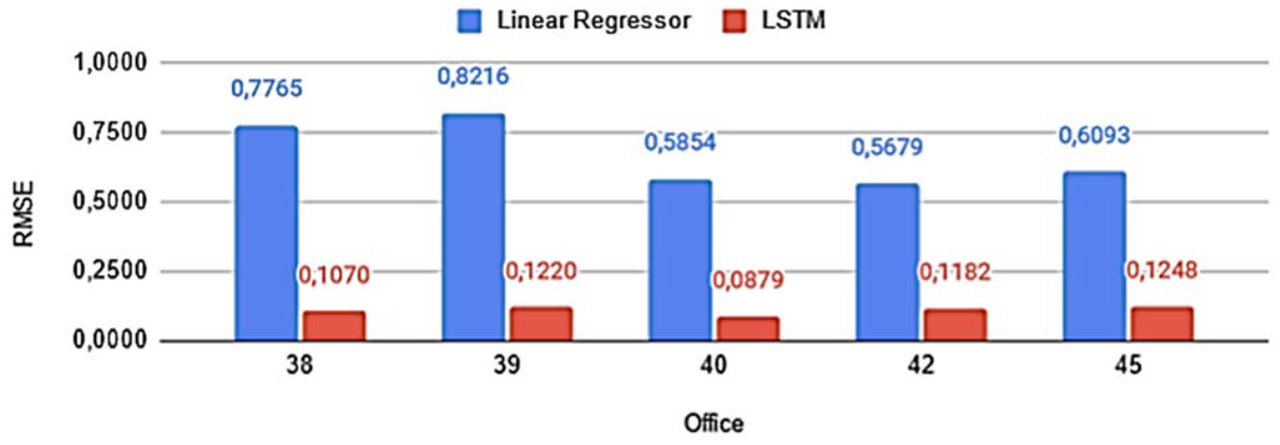
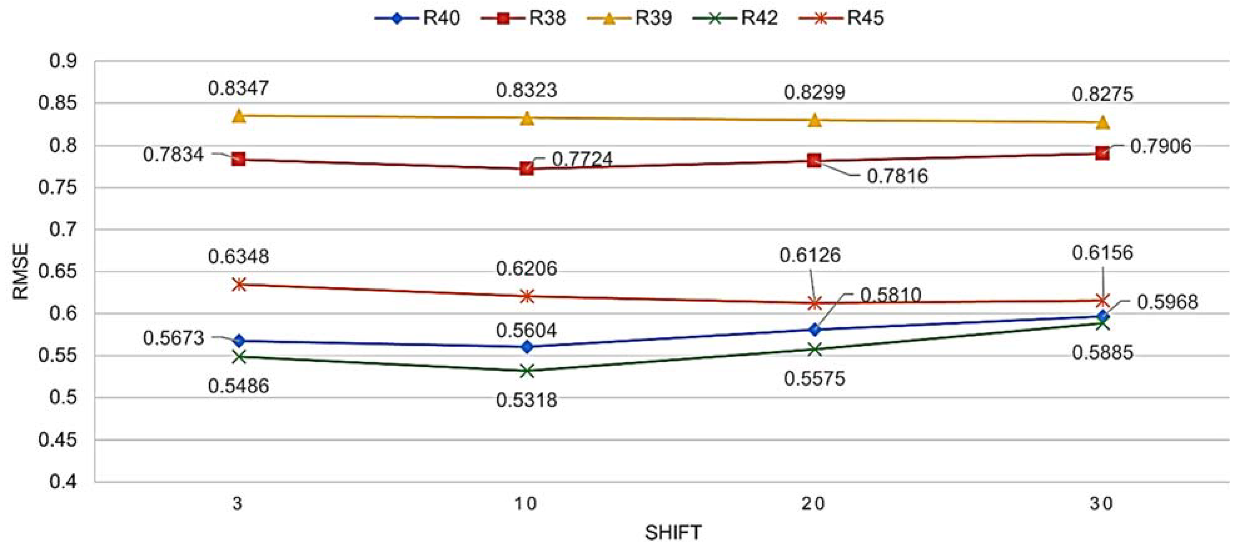
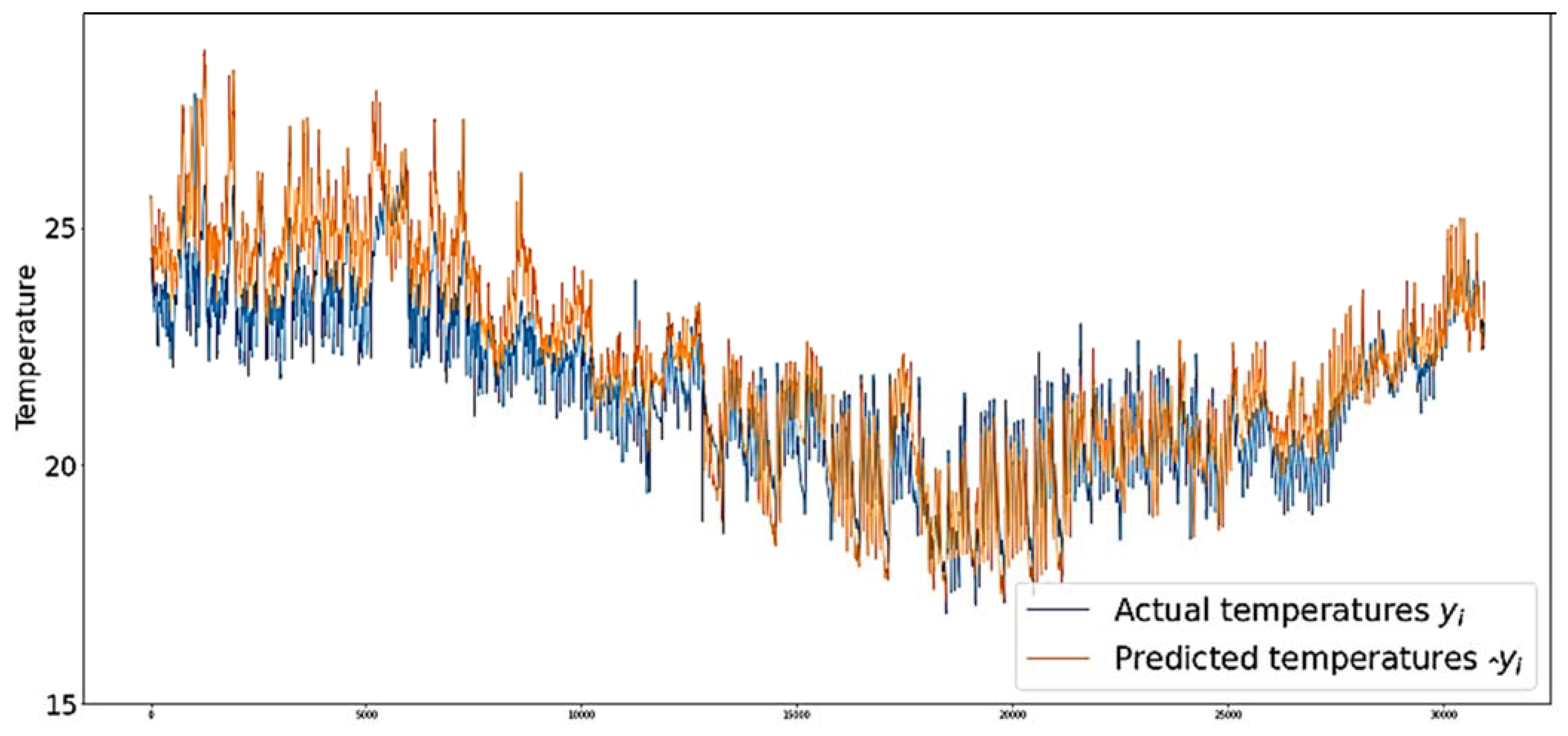
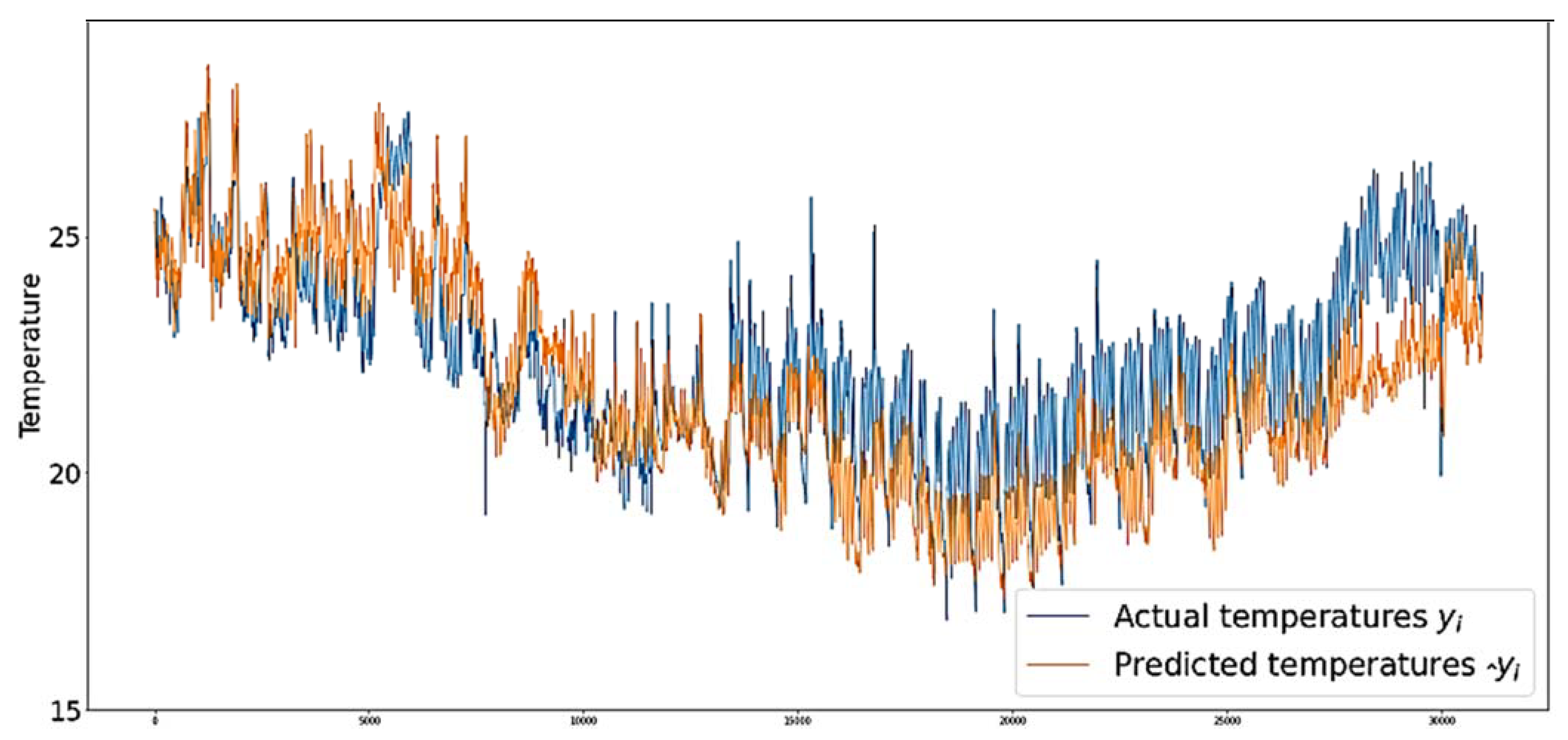
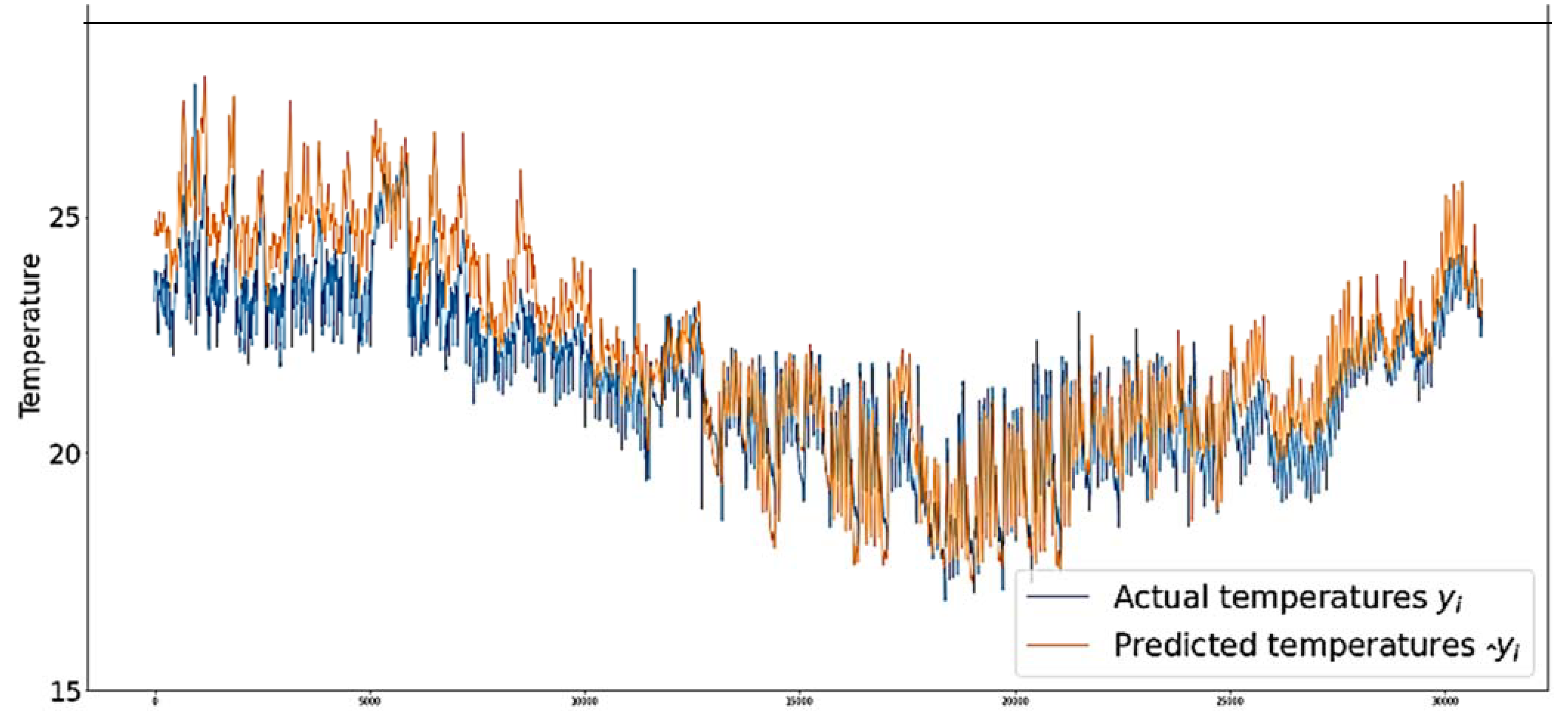
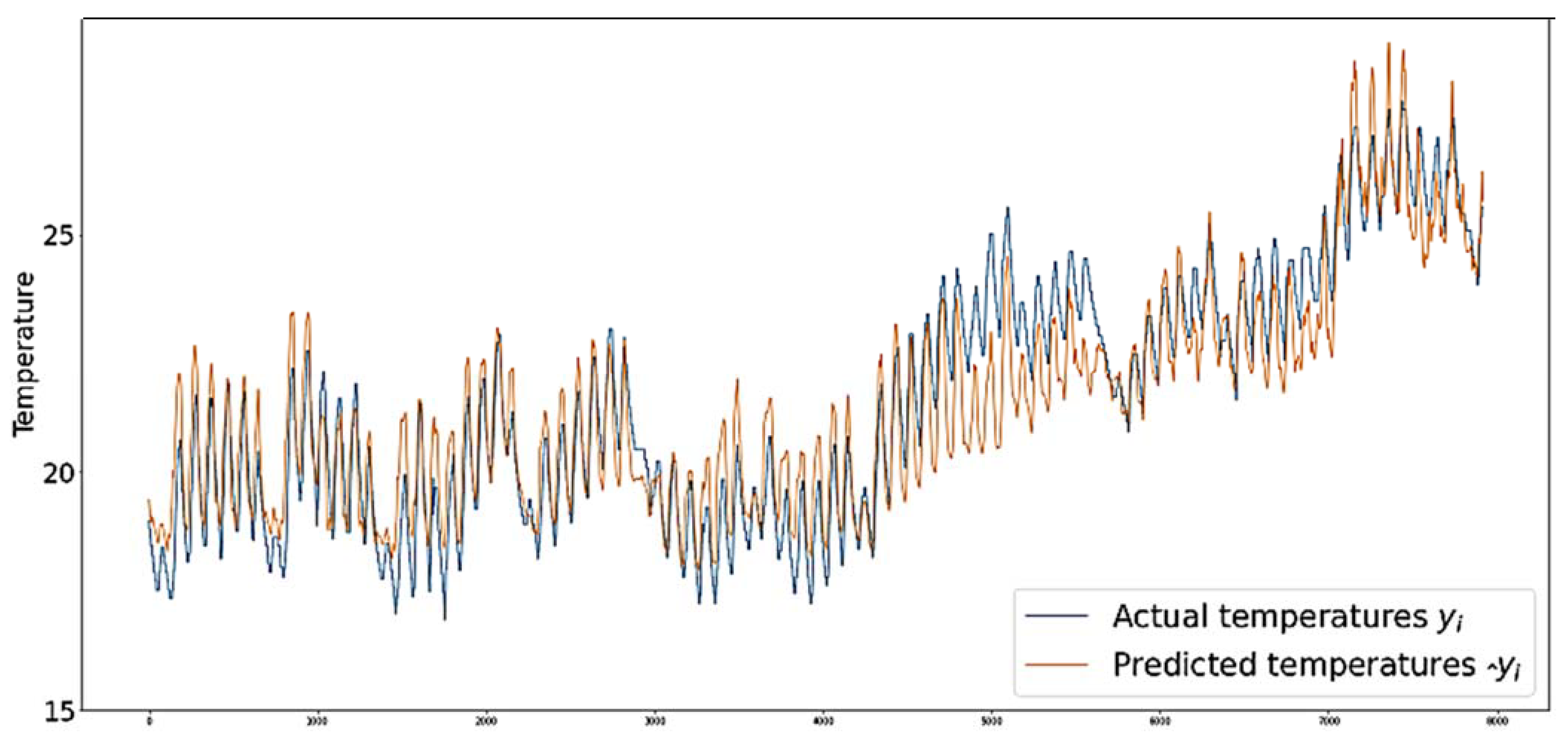
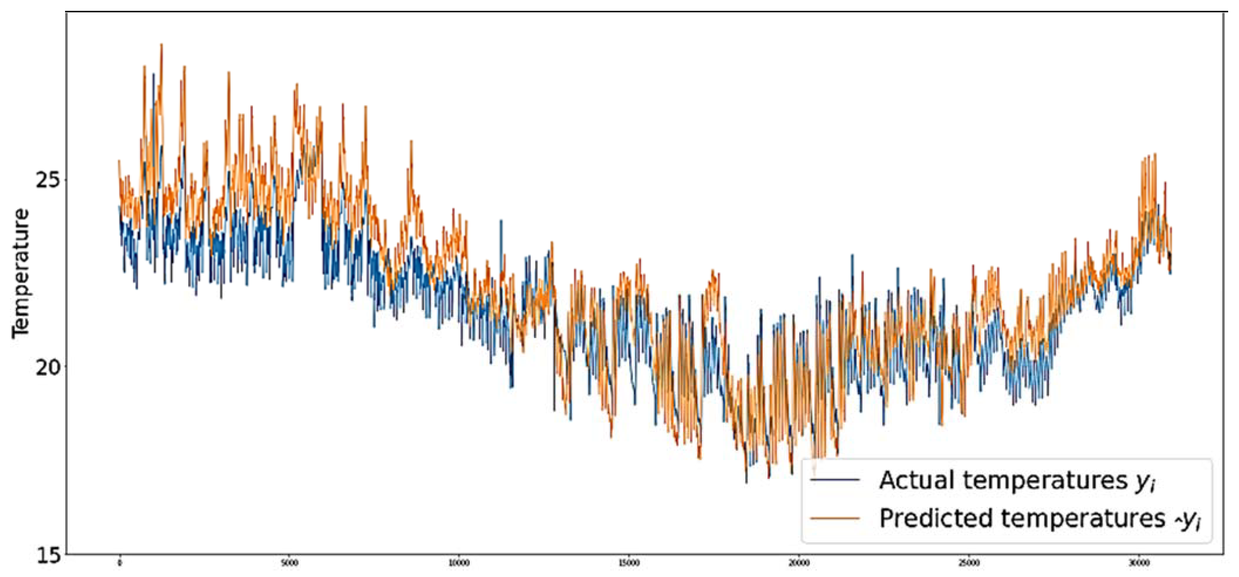
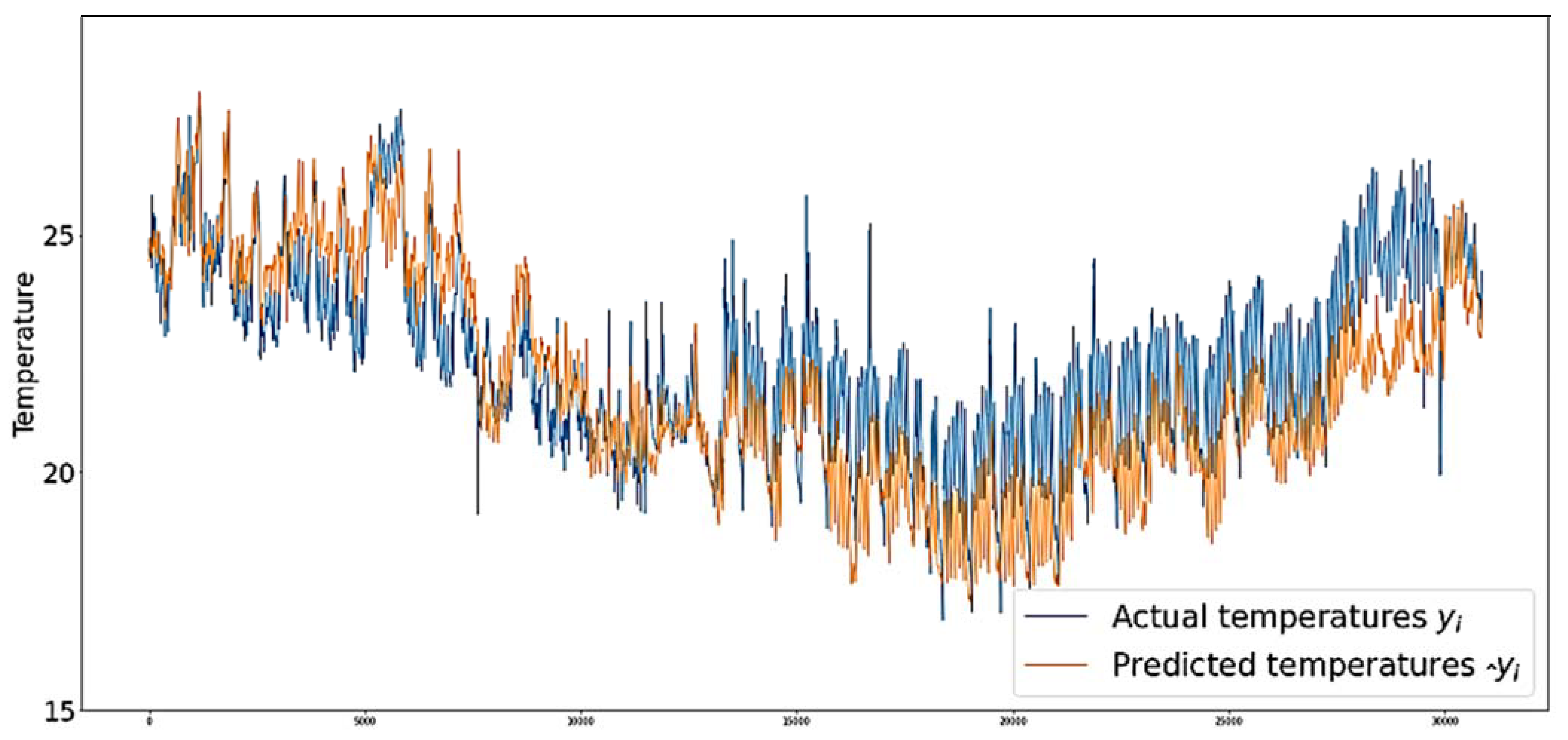
3. Results
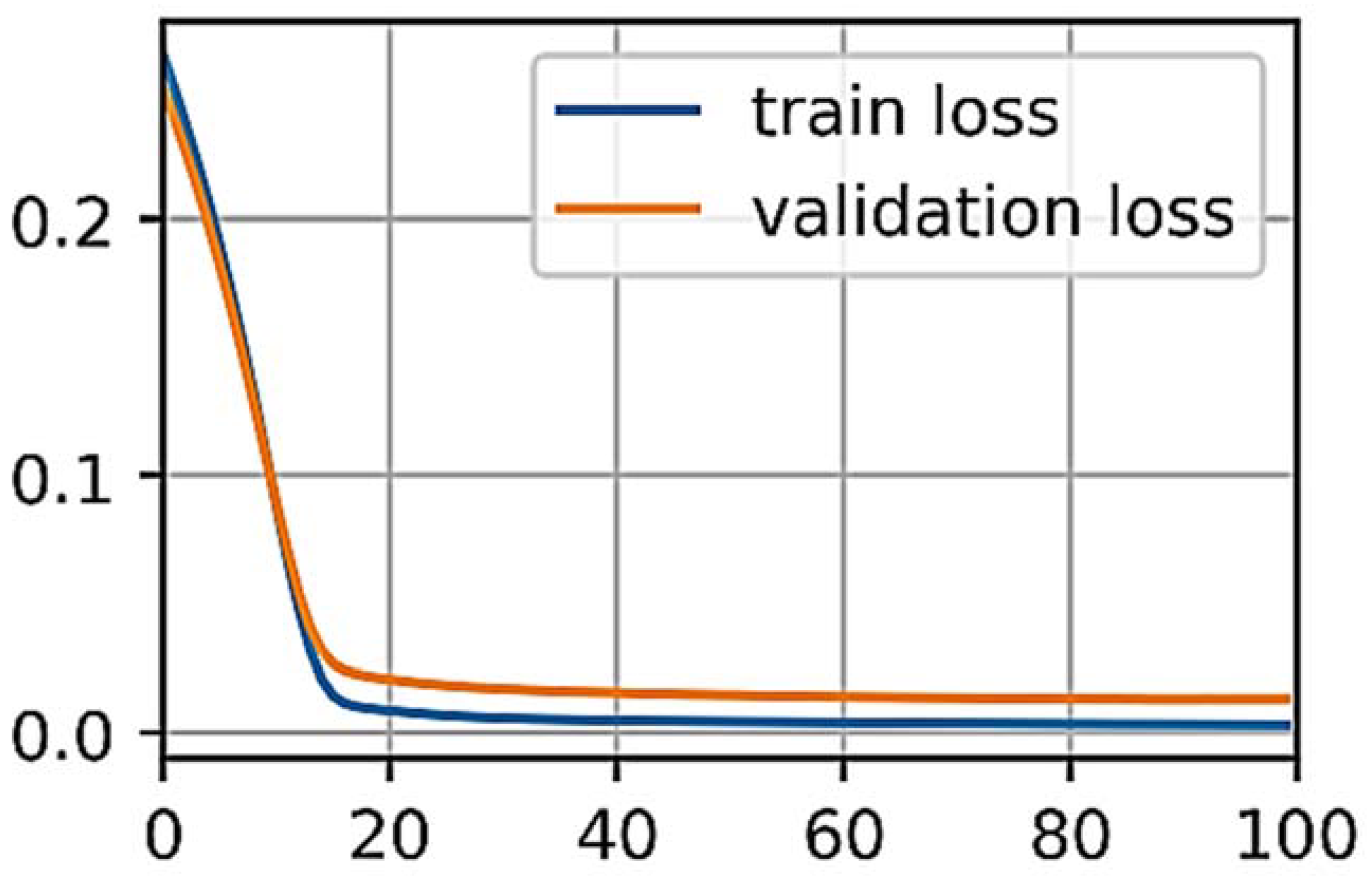
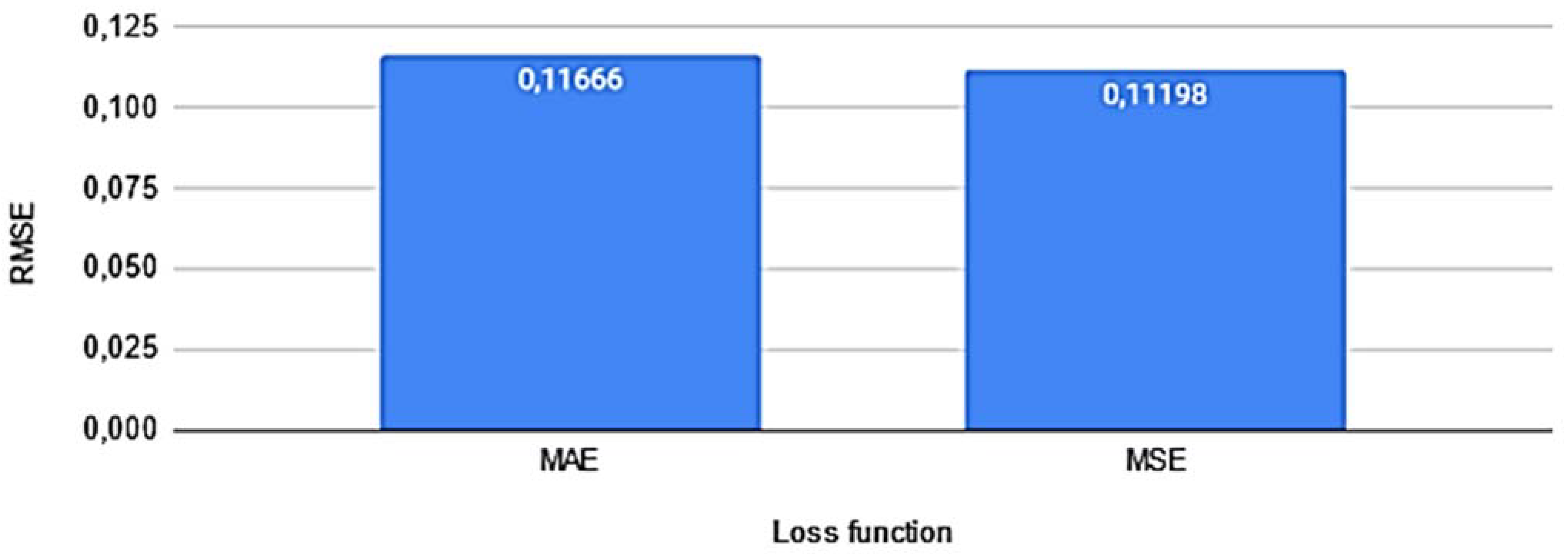
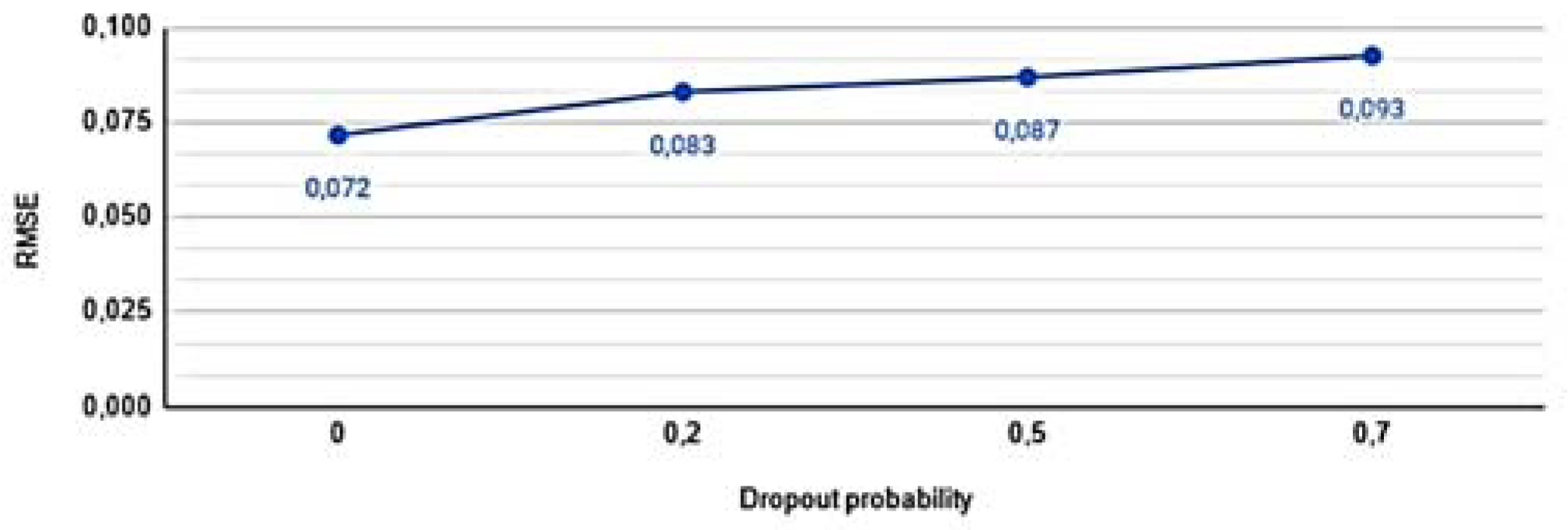
3.1. Model Tuning
3.2. Test
3.3. Tailored Models
4. Discussion
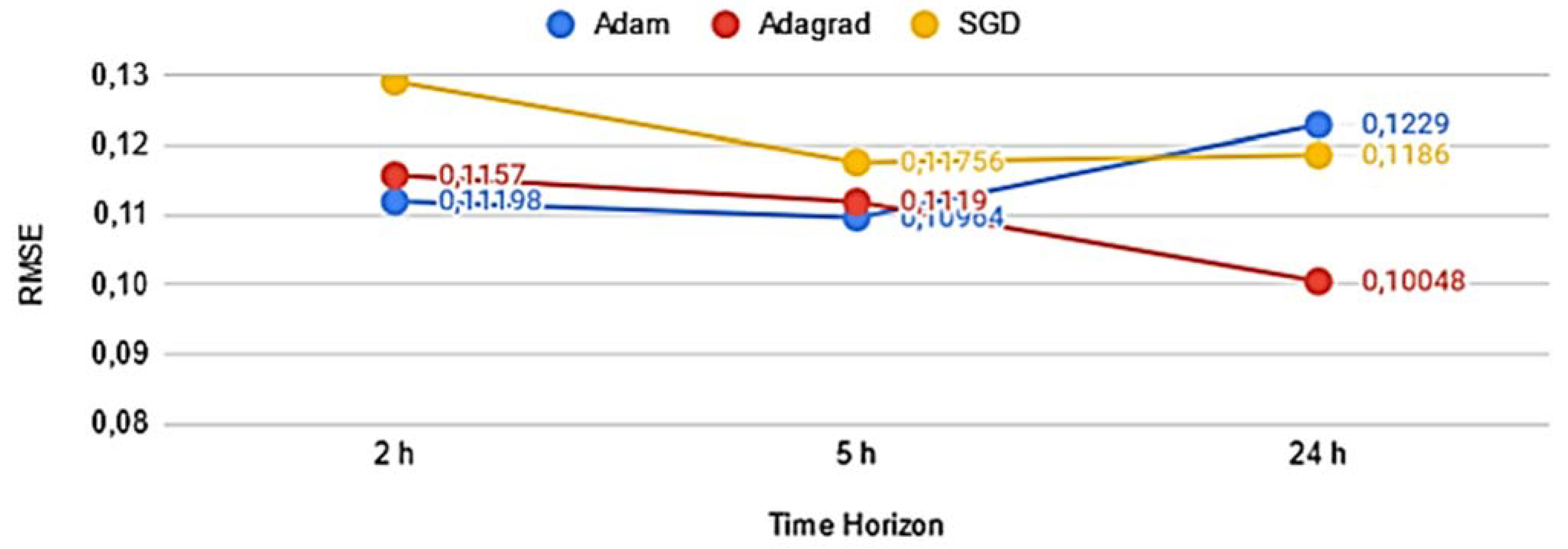
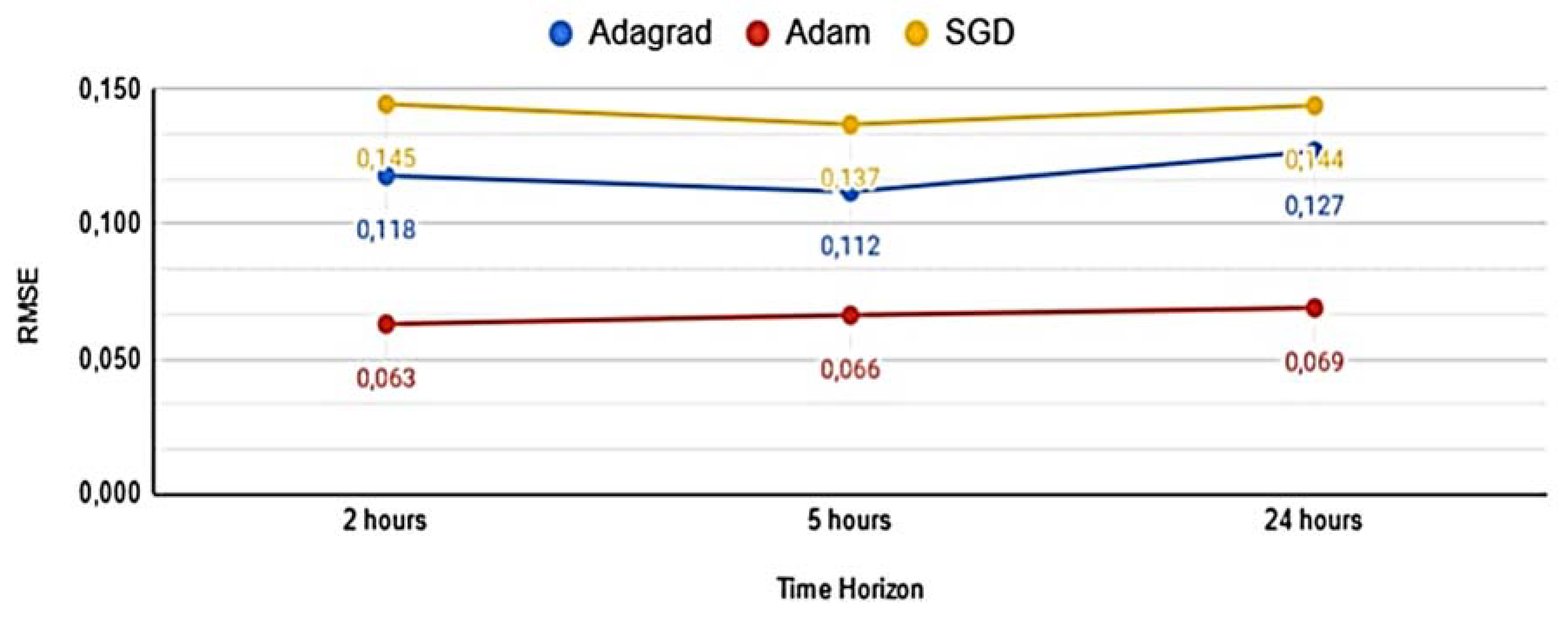
- Increasing the size of the time horizon has a worse impact on the performance of the model if the optimiser is of the type indicated by Adam; the ability to predict variables well in advance would be vital in cases such as prolonged sensor failure, but this type of prediction would be less reliable if the performance of the optimiser is not monitored.
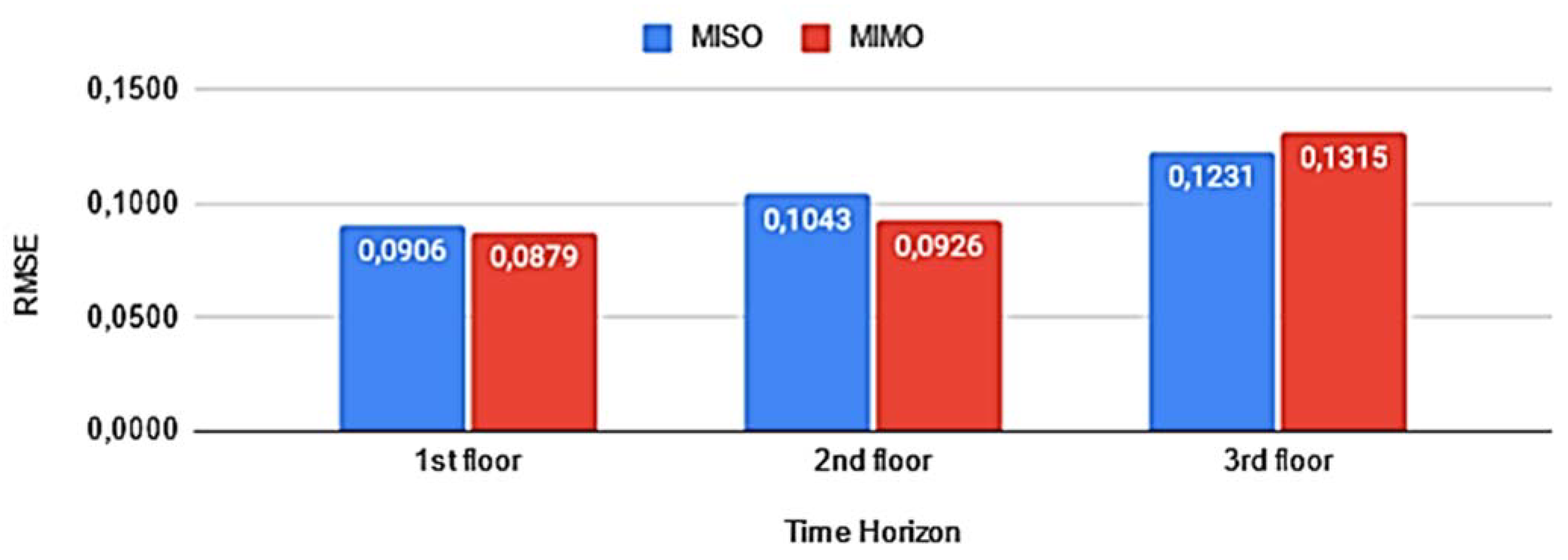
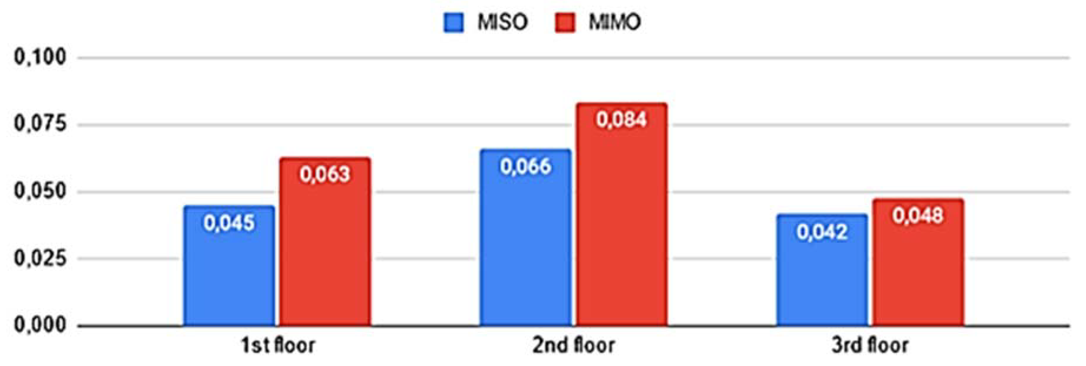
- The MISO scenario does not necessarily guarantee smaller errors in predictions, because it explores a simplified scenario. On the other hand, the MIMO approach ensures completeness in representing the future state of the building. A model that can generalise sufficiently, however, can also achieve better results by running MIMO scenarios, as demonstrated in the Model Tuning subsection and also reported in other similar studies.
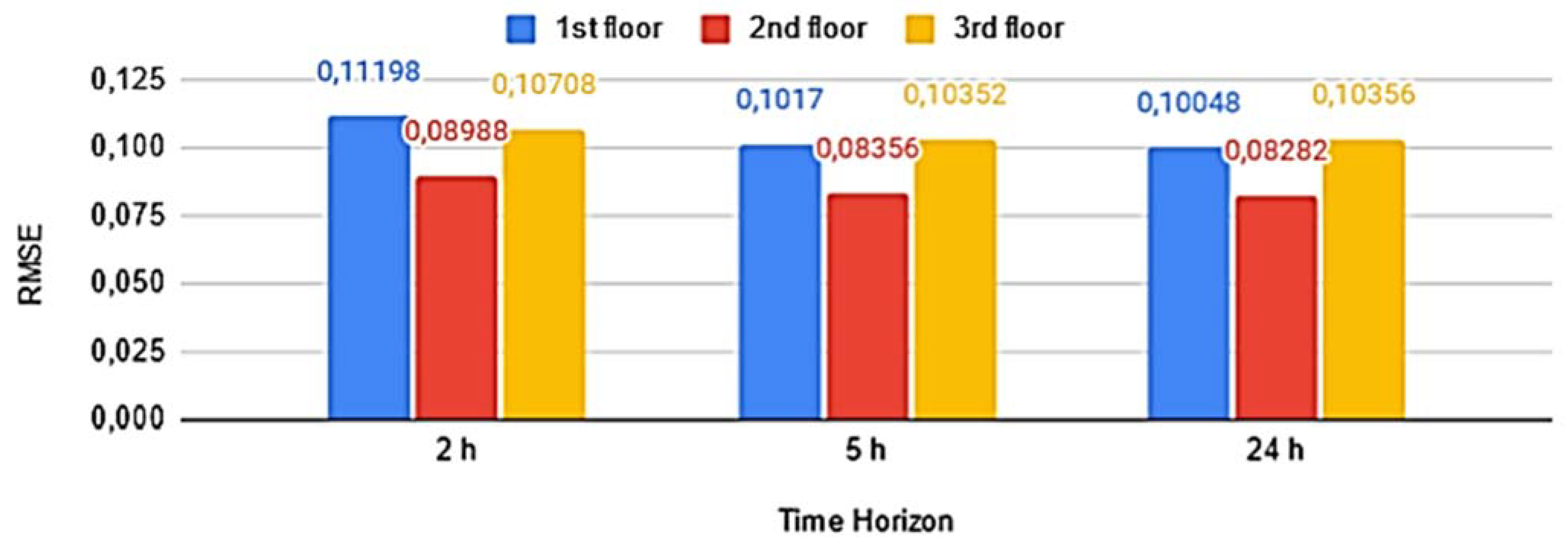
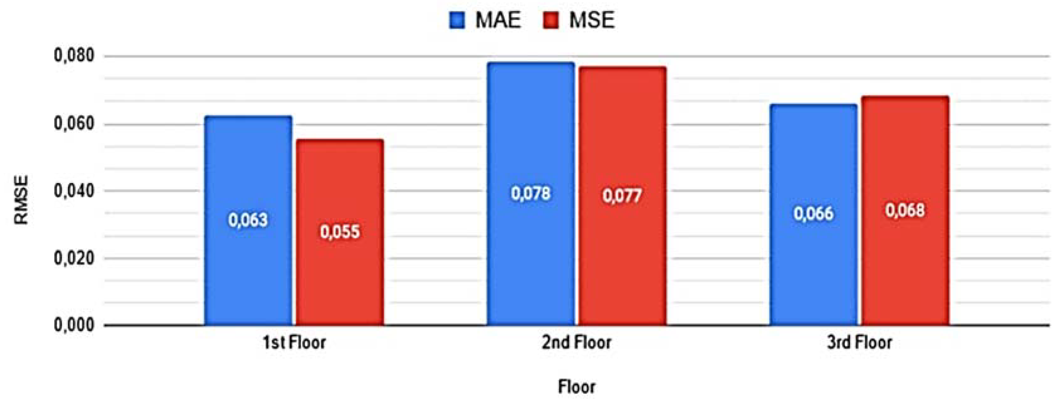
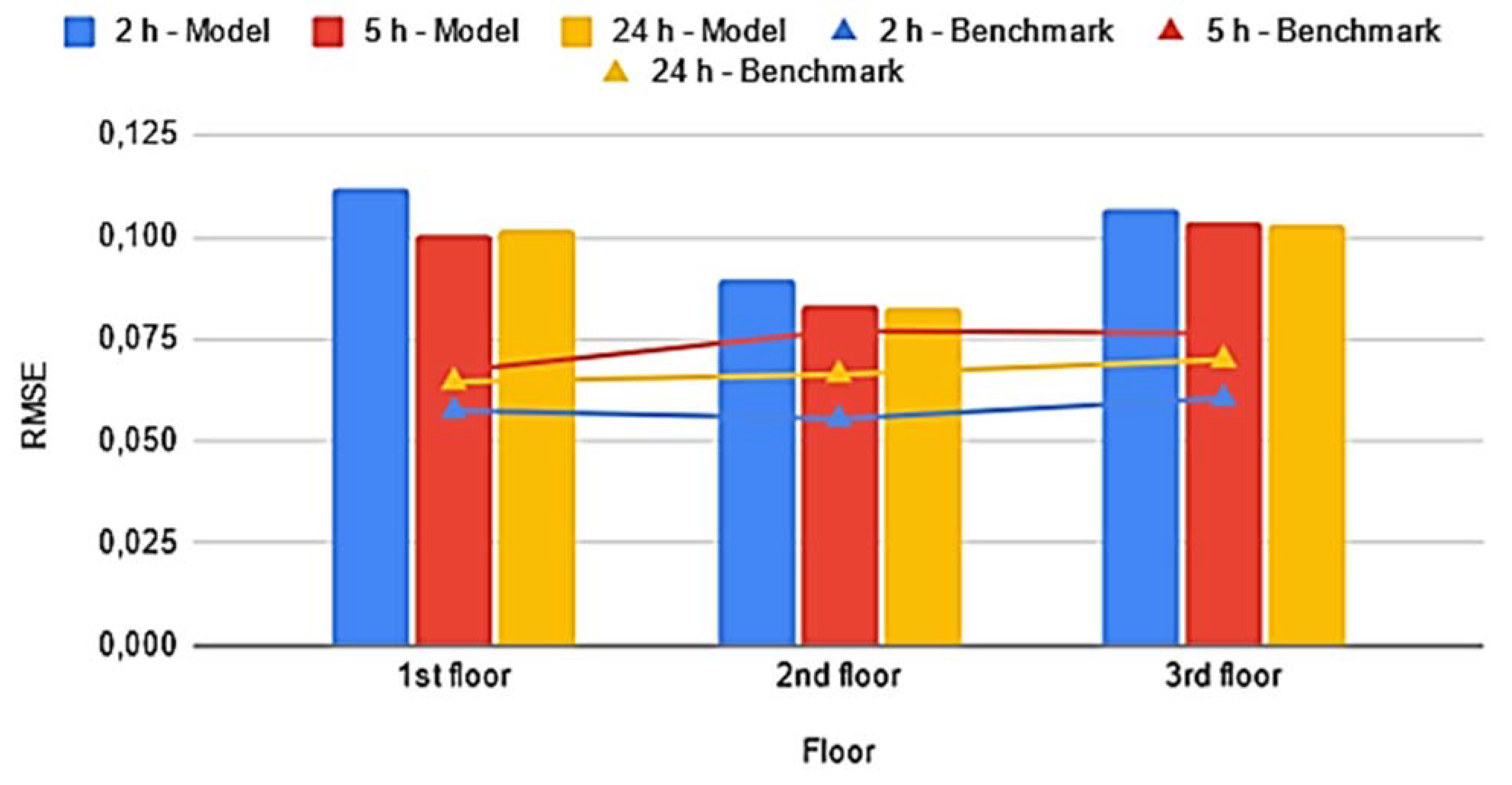
- It must be considered that each floor has different levels of complexity because it is defined by different dynamics. The third floor, for example, has the particularity of the roof, while the second is influenced by the proximity of the other two floors, whose influences are not considered by the input variables. When treating each floor as a single thermal zone, the model’s predictions for the first floor are the most accurate compared to those for the second and third floors, whereas when the model is trained to generalise more, it does not seem to be influenced much by the floor considered.
- The traditional structure works well for short-term forecasts, but performance may deteriorate as the forecast horizon is extended, to the point that for a longer period the two-way structure is preferable; this is the case both considering the plans as separate areas. Thus, the length of the horizon appears to be a parameter that affects performance.
- The chosen learning rate ensures error constancy during the training phase and is very low (i.e., 0.000001); at the same time, since the preferred optimiser is often of the Adam type, known to have the fastest convergence rate, calculation times are not unacceptable, and similarly when the chosen optimiser is of the Adagrad or SGD type.
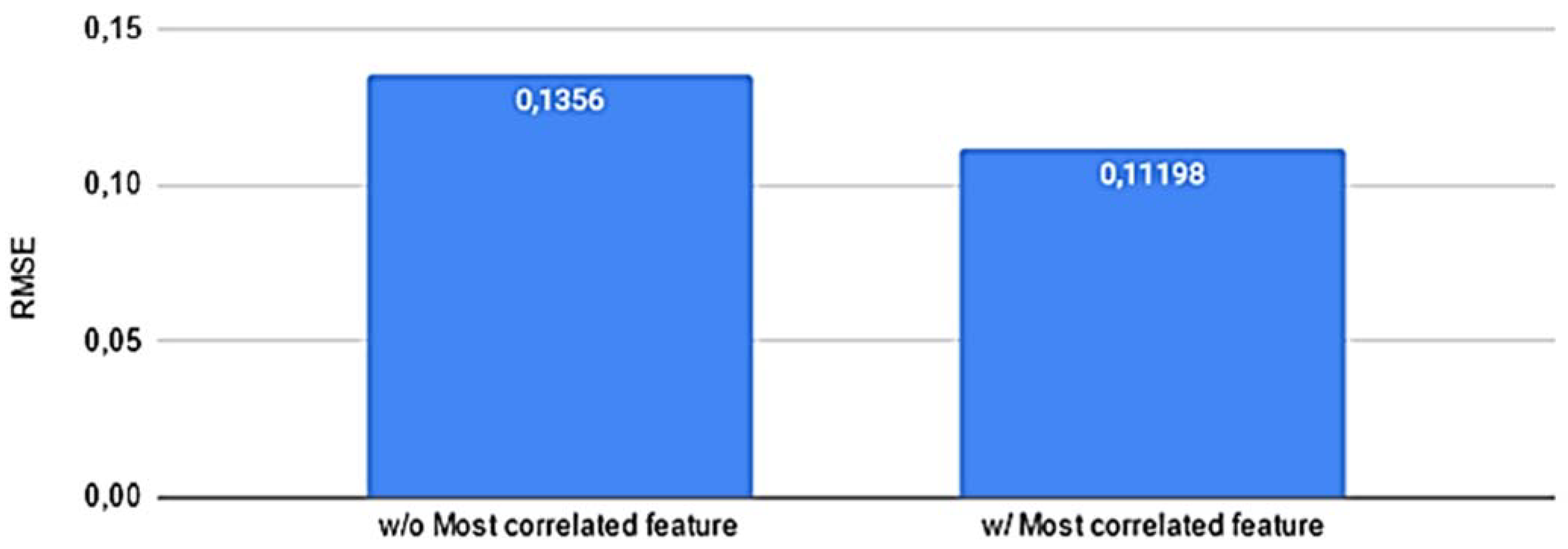
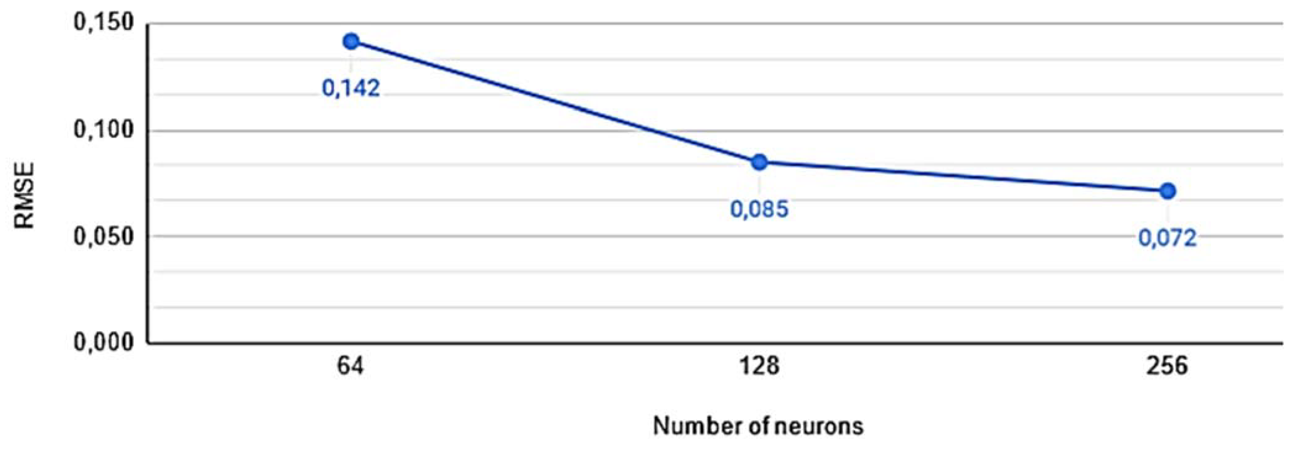
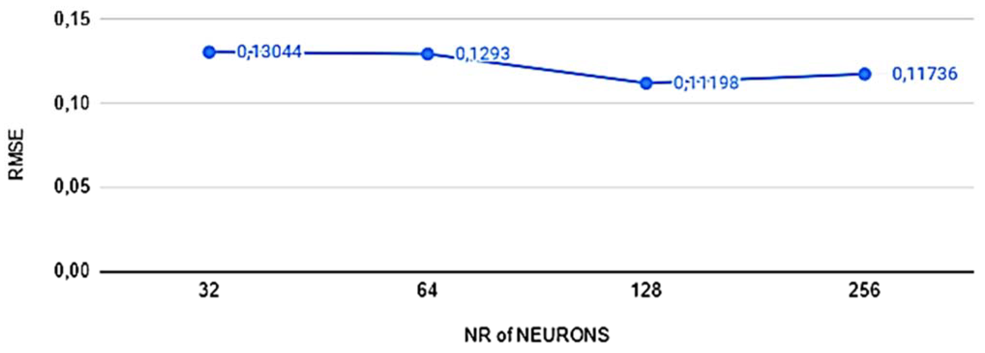
- The highest tested numerosity (i.e., 256 neurons) is the one that guarantees the best performance when the model is perfectly adapted to the reference area as far as possible. Otherwise, a model that must remain versatile may become too complex and the ideal number of neurons is much lower, around 128, resulting in a simpler structure.
Comparison with Similar Studies
5. Conclusions
Author Contributions
Funding
Institutional Review Board Statement
Informed Consent Statement
Data Availability Statement
Acknowledgments
Conflicts of Interest
Nomenclature
| °C | Celsius degree |
| AHU | Air Handling Unit |
| ANN | Artificial Neural Networks |
| ARMA | AutoRegressive Moving Average |
| ARMAX | AutoRegressive Moving Average with eXogenous inputs |
| ARX | AutoRegressive time series with eXogenous inputs |
| avg | average |
| BP | Back Propagation |
| ELM | Extreme Learning Machine |
| EU | European Union |
| h | hour(s) |
| HVAC | Heating Ventilation Air Conditioning |
| LSTM | Long Short-Term Memory |
| MAE | Mean Absolute Error |
| MAEE | Mean Absolute Error Estimation |
| MIMO | Multi Input Multi Output |
| MISO | Multi Input Single Output |
| MSE | Mean Squared Error |
| NARX | Nonlinear AutoRegressive with eXternal input |
| ODE | Ordinary Differential Equation |
| R | correlation index |
| RC | Resistance-Capacitance |
| ReLU | Rectified Linear Unit |
| RMSE | Root Mean Squared Error |
| SVM | Support Vector Machine |
| WRT | With Respect To |
References
- Directive 2010/31/EU Energy Performance Building Directive; European Parliament: Strasbourg, France, 2010.
- Aliberti, A.; Bottaccioli, L.; Macii, E.; Di Cataldo, S.; Acquaviva, A.; Patti, E. A non-linear autoregressive model for indoor air-temperature predictions in smart buildings. Electronics 2019, 8, 979. [Google Scholar] [CrossRef] [Green Version]
- Zhao, H.X.; Magoulès, F. A review on the prediction of building energy consumption. Renew. Sustain. Energy Rev. 2012, 16, 3586–3592. [Google Scholar] [CrossRef]
- Fong, K.F.; Hanby, V.I.; Chow, T.T. HVAC system optimization for energy management by evolutionary programming. Energy Build. 2006, 38, 220–231. [Google Scholar] [CrossRef]
- Foucquier, A.; Robert, S.; Suard, F.; Stéphan, L.; Jay, A. State of the art in building modeling and energy performance prediction: A review. Renew. Sustain. Energy Rev. 2013, 23, 272–288. [Google Scholar] [CrossRef] [Green Version]
- Amara, F.; Agbossou, K.; Cardenas, A.; Dubé, Y.; Kelouwani, S. Comparison and simulation of building thermal models for effective energy management. Smart Grid Renew. Energy 2015, 6, 95–112. [Google Scholar] [CrossRef] [Green Version]
- Fraisse, G.; Viardot, C.; Lafabrie, O.; Achard, G. Development of a simplified and accurate building model based on electrical analogy. Energy Build. 2002, 34, 1017–1031. [Google Scholar] [CrossRef]
- Ramallo-González, A.P.; Eames, M.E.; Coley, D. Lumped parameter models for building thermal modelling: An analytic approach to simplifying complex multi-layered constructions. Energy Build. 2013, 60, 174–184. [Google Scholar] [CrossRef] [Green Version]
- Van Dijk, D. EN ISO 52016 1: The new International Standard to calculate building energy needs for heating and cooling, internal temperature and heating and cooling loads. In Proceedings of the Building Simulation, Rome, Italy, 2–4 September 2019. [Google Scholar]
- Vivian, J.; Zarrella, A.; Emmi, G.; De Carli, M. An evaluation of the suitability of lumped-capacitance models in calculating energy needs and thermal behaviour of buildings. Energy Build. 2017, 150, 447–467. [Google Scholar] [CrossRef]
- Wang, S.; Xu, X. Simplified building model for transient thermal performance estimation using GA-based parameter identification. Int. J. Therm. Sci. 2006, 45, 419–432. [Google Scholar] [CrossRef]
- Braun, J.E.; Chaturvedi, N. An inverse gray-box model for transient building load prediction. HVAC Res. 2002, 8, 73–99. [Google Scholar] [CrossRef]
- Chen, R.T.; Rubanova, Y.; Bettencourt, J.; Duvenaud, D.K. Neural ordinary differential equations. NeurIPS 2018, 31, 6572–6583. [Google Scholar]
- Daw, A.; Karpatne, A.; Watkins, W.; Read, J.; Kumar, V. Physics-guided neural networks (PGNN): An application in lake temperature modeling. arXiv 2017, arXiv:1710.11431. [Google Scholar]
- Massano, M.; Patti, E.; Macii, E.; Acquaviva, A.; Bottaccioli, L. An online gray-box model based on unscented Kalman filter to predict temperature profiles in smart buildings. Energies 2020, 13, 2097. [Google Scholar] [CrossRef]
- Hermawan, P.E. Indoor temperature prediction of the houses with exposed stones in tropical mountain regions during four periods of different seasons. Int. J. Civ. Eng. Technol. 2019, 10, 604–612. [Google Scholar]
- Soleimani-Mohseni, M.; Thomas, B.; Fahlén, P. Estimation of operative temperature in buildings using artificial neural networks. Energy Build. 2006, 18, 635–640. [Google Scholar] [CrossRef]
- Lu, T.; Viljanen, M. Prediction of indoor temperature and relative humidity using neural network models: Model comparison. Neural Comput. Applic 2009, 18, 345. [Google Scholar] [CrossRef]
- Mba, L.; Meukam, P.; Kemajou, A. Application of artificial neural network for predicting hourly indoor air temperature and relative humidity in modern building in humid region. Energy Build. 2016, 121, 32–42. [Google Scholar] [CrossRef]
- Shi, X.; Lu, W.; Zhao, Y.; Qin, P. Prediction of indoor temperature and relative humidity based on cloud database by using an improved BP neural network in Chongqing. IEE Access 2018, 6, 30559–30566. [Google Scholar] [CrossRef]
- Attoue, N.; Shahrour, I.; Younes, R. Smart building: Use of the artificial neural network approach for indoor temperature forecasting. Energies 2018, 11, 395. [Google Scholar] [CrossRef] [Green Version]
- Xu, C.; Chen, H.; Wang, J.; Guo, Y.; Yuan, Y. Improving prediction performance for indoor temperature in public buildings based on a novel deep learning method. Build. Environ. 2019, 148, 128–135. [Google Scholar] [CrossRef]
- Huang, H.; Chen, L.; Hu, E. A neural network-based multi-zone modelling approach for predictive control system design in commercial buildings. Energy Build. 2015, 97, 86–97. [Google Scholar] [CrossRef]
- Fang, Z.; Crimier, N.; Scanu, L.; Midelet, A.; Alyafi, A.; Delinchant, B. Multi-zone indoor temperature prediction with LSTM-based sequence to sequence model. Energy Build. 2021, 245, 111053. [Google Scholar] [CrossRef]
- Li, Q.; Meng, Q.; Cai, J.; Yoshino, H.; Mochida, A. Applying support vector machine to predict hourly cooling load in the building. Appl. Energy 2009, 86, 2249–2256. [Google Scholar] [CrossRef]
- Noorazizi, M.S.; Zaki, S.A.; Abdullah, S.S. Black box modelling and simulating the dynamic indoor air temperature of a laboratory using ARMA model. Indones. J. Electr. Eng. Comput. Sci. 2020, 21, 791–800. [Google Scholar]
- Afroz, Z.; Shafiullah, G.; Urmee, T.; Higgins, G. Prediction of Indoor Temperature in an Institutional Building. Energy Procedia 2017, 142, 1860–1866. [Google Scholar] [CrossRef]
- Mateo, F.; Carrasco, J.J.; Sellami, A.; Millán-Giraldo, M.; Domínguez, M.; Olivas, E.S. Machine learning methods to forecast temperature in buildings. Expert Syst. Appl. 2013, 40, 1061–1068. [Google Scholar] [CrossRef]
- Mustafaraj, G.; Lowry, G.; Chen, J. Prediction of room temperature and relative humidity by autoregressive linear and non-linear neural network models for an open office. Energy Build. 2011, 43, 1452–1460. [Google Scholar] [CrossRef]
- Gustin, M.; McLeod, R.S.; Lomas, K.J. Forecasting indoor temperatures during heatwaves using time series models. Build. Environ. 2018, 143, 727–739. [Google Scholar] [CrossRef]
- Alawadi, S.; Mera, D.; Fernández-Delgado, M.; Alkhabbas, F.; Olsson, C.M.; Davidsson, P. A comparison of machine learning algorithms for forecasting indoor temperature in smart buildings. Energy Syst. 2020, 1–17. [Google Scholar] [CrossRef] [Green Version]
- Dabas, N.; Singh, R.P. ELM-Kernel and reduced kernel ELM based watermarking scheme. J. Inf. Secur. Appl. 2019, 46, 173–192. [Google Scholar] [CrossRef]


| Description | Unit of Measurement |
|---|---|
| Ceiling conditioning panel supply temperature | °C |
| Return temperature of cold collector supplying ceiling conditioning panels | °C |
| Supply temperature of cold collector supplying ceiling conditioning panels | °C |
| AHU supply temperature for the whole considered building area | °C |
| Return temperature of hot collector supplying ceiling conditioning panels | °C |
| Supply temperature of hot collector supplying ceiling conditioning panels | °C |
| Target floor AHU supply humidity degree | Int |
| Target floor AHU return humidity degree | Int |
| Target floor AHU supply temperature | °C |
| Target floor AHU return temperature | °C |
| Outdoor temperature | °C |
| Target office setpoint temperature | °C |
| Target office indoor temperature | °C |
| Hour of the day | Int |
| Dataset | Percentage | Records |
|---|---|---|
| Training set | Around 70% | Around 23,000 (i.e., 9 months of observations from first floor) |
| Validation set | Around 30% | Around 4000 (i.e., 2 months of observations from first floor) |
| First Test Set | 100% | Around 23,000 (i.e., 11 months of observations from second floor) |
| Second Test Set | 100% | Around 23,000 (i.e., 11 months of observations from third floor) |
| Dataset | Percentage | Records |
|---|---|---|
| Training set | Around 70% | Around 23,000 (i.e., 8 months of observations) |
| Validation set | Around 15% | Around 4000 (i.e., 1–5 months of observations) |
| Test set | Around 15% | Around 4000 (i.e., 1–5 months of observations) |
| Office and Prediction Horizon | 2 h | 5 h | 24 h |
|---|---|---|---|
| P1-R40 | 0.0879 | 0.0878 | 0.0771 |
| P1-R38 | 0.1070 | 0.0942 | 0.0945 |
| P1-R39 | 0.1220 | 0.1086 | 0.1011 |
| P1-R42 | 0.1182 | 0.1108 | 0.1120 |
| P1-R45 | 0.1248 | 0.1071 | 0.1177 |
| P2-R40 | 0.0926 | 0.0920 | 0.0900 |
| P2-R38 | 0.0875 | 0.0801 | 0.0836 |
| P2-R39 | 0.0902 | 0.0817 | 0.0914 |
| P2-R42 | 0.0846 | 0.0717 | 0.0721 |
| P2-R45 | 0.0945 | 0.0886 | 0.0807 |
| P3-R40 | 0.1315 | 0.1291 | 0.1245 |
| P3-R38 | 0.0768 | 0.0789 | 0.0806 |
| P3-R39 | 0.1594 | 0.1571 | 0.1650 |
| P3-R42 | 0.0785 | 0.0689 | 0.0726 |
| P3-R45 | 0.0892 | 0.0836 | 0.0751 |
Publisher’s Note: MDPI stays neutral with regard to jurisdictional claims in published maps and institutional affiliations. |
© 2022 by the authors. Licensee MDPI, Basel, Switzerland. This article is an open access article distributed under the terms and conditions of the Creative Commons Attribution (CC BY) license (https://creativecommons.org/licenses/by/4.0/).
Share and Cite
Di Già, S.; Papurello, D. Hybrid Models for Indoor Temperature Prediction Using Long Short Term Memory Networks—Case Study Energy Center. Buildings 2022, 12, 933. https://doi.org/10.3390/buildings12070933
Di Già S, Papurello D. Hybrid Models for Indoor Temperature Prediction Using Long Short Term Memory Networks—Case Study Energy Center. Buildings. 2022; 12(7):933. https://doi.org/10.3390/buildings12070933
Chicago/Turabian StyleDi Già, Silvia, and Davide Papurello. 2022. "Hybrid Models for Indoor Temperature Prediction Using Long Short Term Memory Networks—Case Study Energy Center" Buildings 12, no. 7: 933. https://doi.org/10.3390/buildings12070933
APA StyleDi Già, S., & Papurello, D. (2022). Hybrid Models for Indoor Temperature Prediction Using Long Short Term Memory Networks—Case Study Energy Center. Buildings, 12(7), 933. https://doi.org/10.3390/buildings12070933