Detecting Damage Evolution of Masonry Structures through Computer-Vision-Based Monitoring Methods

Abstract

Detecting the onset of structural damage and its progressive evolution is crucial for the assessment and maintenance of the built environment. This paper describes the application of a computer-vision-based methodology for structural health monitoring to a shake table investigation. Three rubble stone masonry walls, one unreinforced and two reinforced, were tested under natural earthquake base inputs, progressively scaled up to collapse. White noise signals were also applied for dynamic identification purposes. Throughout the experiments, videos were recorded, under both white noise excitation and environmental vibrations, with the table at rest. The videos were preprocessed with motion magnification algorithms and analyzed through a principal component analysis. The natural frequencies of the walls were detected and their progressive decay was associated with damage accumulation. Results agreed with those obtained from another measurement system available in the laboratory and were consistent with the crack pattern development surveyed during the tests. The proposed approach proved useful to derive information on the progressive deterioration of the structural properties, showing the feasibility of this methodology for real field applications.

1. Introduction

Existing masonry and historic buildings have usually sustained loads and exceptional actions, such as earthquakes, for many decades, sometimes even centuries or millennia. This time span is well beyond the service life they had likely been originally conceived for and, to ensure their safety conditions, maintenance has to be efficiently programmed and performed.

Actual structural health conditions thus need to be assessed to prioritize interventions and to monitor possible changes in the structural performance of the building stock. Most of the times, non-destructive techniques (NDTs) are preferred as the means by which a structure can be inspected without affecting its serviceability. Many NDTs are based on visual observations or on the evaluation of material properties. Others relate structural conditions to the observed change of the global behavior of the structure through a combination of measurements of either static or dynamic quantities. The use of vibration test data to determine natural frequencies and modal shapes can be referred to in this last group.

The problem of vibration-based damage detection has been dealt with for long time in the scientific community [1,2,3,4]. Nevertheless, during the last decades, many innovative technologies as well as optimized sensors-placing criteria have emerged, allowing more and more sustainable and extensive monitoring campaigns [5,6]. Dynamic monitoring can be performed under either seismic or ambient excitation (usually due to wind, traffic, etc.) with the main objective of estimating modal parameters. A periodic observation of these measurements and/or a comparison with the expected structural behavior, determined through numerical or analytical models, can provide a warning of altered conditions that may compromise structural safety. These monitoring techniques, routinely performed with physically attached wired or wireless sensors (accelerometers or vibrometers) have, however, some intrinsic limitations related to the number of sensors that can be placed on the structure, their cost, maintenance, and, sometimes, the accessibility of the structure itself.

To cope with these issues and to overcome some of the above-mentioned drawbacks, computer vision (CV)-based structural dynamics techniques have emerged and have demonstrated clear advantages in terms of cost, speed, and spatial resolution. Nowadays, CV-based techniques have been intensively explored for the extraction of modal parameters, measuring displacement time histories by determining the relative position of a structure throughout time [7,8,9,10,11,12].

Referring to CV-based structural dynamics, techniques for motion magnification (MM) [13] have been introduced to emphasize and visualize small motions from video measurements [14,15]. Such preprocessing stage is not only indispensable when dealing with imperceptible structural vibrations due to traffic or wind, but, as it will be further explained, it is also a filtering expedient. While in the literature some applications of these techniques on historic masonry structures have already been proposed [14], the novelty of this study lies in the adoption of principal component analysis to extract the main components related to the natural frequency of the structure. This work also provides a systematic comparison with other monitoring techniques, and, namely, with an optical system making use of infrared cameras and retro-reflective markers. Finally, relying on the measurements recorded during a number of tests on different specimens characterized by different damage states, the work investigates the application of the technique as a means to detect possible seismic induced damage.

In fact, in the context of historic masonry buildings, monitoring is being employed with a twofold aim, that is, as a diagnosis tool and as a control tool, and it is recognized as pivotal throughout the entire preservation process [16,17,18]. Looking at the damage caused to masonry structures by earthquakes or simply due to natural deterioration, it is essential to set up tools to monitor the evolution of cracking and possibly detect early warning signs of irreversible changes of structural safety conditions. For such purpose, it is crucial to rely on noninvasive techniques and fast elaboration tools.

To this end, dynamic identification performed via non-contact CV-based tools is a very promising alternative to traditional measurements, since dense and continuous points can be followed and their position can be tracked during time, determining dynamic properties of the structure (i.e., natural frequencies and mode shapes), which are extremely sensitive to any mass or stiffness changes induced by damage [19].

In the following sections, the methodology is presented (Section 2), which was set up and implemented in a Matlab code, taking the motion magnification stage on its phase-based version (PBMM) from the work by Wadhwa et al. [13] and performing a principal component analysis (PCA) to reduce the number of significant motion components to extract the dynamic properties of the structure. Then, in Section 3, the case study on which the methodology was applied is presented, consisting of three rubble stone masonry walls tested on a shake table under both artificial white noise excitation and strong motion earthquake inputs, for which damage progressively advanced up to the collapse. Throughout the experimental investigation, several videos were recorded and analyzed with the proposed technique. In Section 4, the results are compared, in terms of detected frequencies, with those of a monitoring technique adopted in the laboratory for consistent input excitation. In addition, a damage index was calculated and its evolution is related with the progressive development of damage surveyed during the tests and with a visible change of the shape of the hysteresis cycles as well as with the progressive increase of the hysteretic energy. Finally, based on such comparisons, Section 5 reports the advantages of the proposed CV-based method within a more comprehensive discussion in the perspective of its future applications to real structures.

2. Methodology

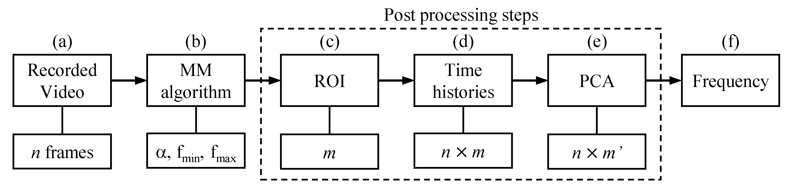
The CV-based methodology is summarized in the flowchart in Figure 1. The video recording (a) and the motion magnification step (b) precede the semi-automated post-processing ones, which start from the selection of an appropriate region of interest (ROI) (c) within the video frames, in which, in general, a parameter considered as representative of the motion of the structure is monitored and tracked during time. This procedure can be followed considering either the motion of a pixel or, as in this case, the evolution of its gray intensity throughout the test (intensity variation). The time histories are then collected and analyzed to identify the dynamic properties of the structure. Having extracted several time histories (d) of the gray intensity for a number of pixels (m), a PCA (e) is performed to reduce the dimensionality of the data and, consequently, to reduce the number of time series ($m^{\prime }<m$) to be analyzed in the frequency domain (f).

It is worth underlying that, differently from laboratory tests, structures in natural environments might exhibit imperceptible vibrations, not detectable unless MM algorithms are applied on the recorded video prior to any other post-processing step. Thus, a MM step (b) should be, in case, introduced right after the video recording in the chart. The MM algorithm in its phase-based version [13] was used in this study and its main features are summarized in the following. MM allows to evaluate and modify, through an amplification factor $\alpha$, local motions on video sequences. This step is fundamental, especially when dealing with videos in which displacement is not visible and, consequently, hardly detectable. The aim is to amplify small motions, within a given range of frequencies (bandpass filtering with predefined high-pass $f_{min}$ and low-pass $f_{max}$ frequencies), without distorting the video sequences.

In its simplest form, considering the 1D translational case and defining $I(x,0)=f\left(x\right)$ as the image gray intensity at the first instant and at the position x, at the generic instant t, the coordinate x can be subjected to a displacement, $\delta$, and the intensity I to a change, obtaining

$$I(x,t)=f(x+\delta (t\left)\right)$$

(1)

which, approximated in a first-order expansion, leads to

$$I(x,t)\approx f\left(x\right)+\delta \left(t\right)\frac{\partial f\left(x\right)}{\partial x}$$

(2)

Applying a temporal band-pass filter ($f_{min}$, $f_{max}$) to $I(x,t)$, and assuming that the motion signal $\delta \left(t\right)$ lies within the defined domain, an amplification factor $\alpha$ can be applied and the processed magnified intensity can be written as

$$\widehat{I}(x,t)\approx f\left(x\right)+(1+\alpha )·\delta \left(t\right)\frac{\partial f\left(x\right)}{\partial x}$$

(3)

Nonetheless, depending on the magnitude of the amplification factor $\alpha$, the application of MM may introduce an additional and artificial noise to the video. Hence, for example, attention should be paid to light condition during video recording, or to possible vibrations of the camera support. The reader is referred to [13] for a more detailed description of the steps characterizing the PBMM algorithm.

Once the MM analysis is conducted, a new magnified video will be generated and then analyzed in the later steps.

It is known that each pixel of a grayscaled image can be characterized by its intensity, i.e., a measure of the amount of light that can range from 0 (black) to 255 (white). According to the methodology proposed, defining n as the number of frames composing the video sequence, the video is first converted in grayscale frames so that each pixel of the single frame, identified by its coordinates $x_k$ and $y_k$, is characterized by an intensity value $I(x_k,y_k)$. This latter is also a function of time t, each time instant corresponding to a frame. Monitoring the variation of intensity during time provides a series of time histories, each referred to a pixel, which can be considered as representative of the motion, captured through the variation in colour/light of a number of sensors that corresponds to the dimension of the selected ROI. One possible solution for ROI selection is provided by [14], based on the evaluation of the entropy of the images, and it is the one adopted in this study. The average local entropy is a statistical measure of randomness, which can be used to characterize the contrast of an input image: focusing on a single pixel, high entropy means that the selected pixel has a low probability of having, in its neighborhood, pixels with the same gray intensity. Hence, pixels with high entropy can be better visualized and their intensity variation can be better caught by the computer vision technique. This choice also entails a high signal-to-noise ratio for the selected region. The average local entropy ($\overline{E}$) of the k-th pixel is defined in this context as

$$\overline{E}(x_k,y_k)=\frac{{\displaystyle \sum _{i=1}^n}-\left({\displaystyle \sum _z}p\left(x_k,y_k\right){log}_{2}p\left(x_k,y_k\right)\right)}{n}$$

(4)

where n is the number of the frames and $p(x_k,y_k)$ is the normalized histogram counts of the grayscale intensities evaluated in a $9\times 9$ square “neighborhood” of the pixel k (z is the number of pixels analyzed within the $9\times 9$ pixels neighborhood). The ROI, therefore, can be selected choosing areas with higher local entropy values. Once the ROI of dimension $b\times h$ is selected, the total number of pixels to be monitored is $m=b·h$, and a matrix $\mathbf{T}$ collecting, by column, the m time histories of the gray intensity made up of n instants/frames can be assembled and then post-processed

$$\mathbf{T}=\left[\begin{array}{cccccc}{\mathbf{T}}_{\mathbf{1}}& {\mathbf{T}}_{\mathbf{2}}& \dots & {\mathbf{T}}_{\mathbf{k}}& \dots & {\mathbf{T}}_{\mathbf{m}}\end{array}\right]$$

(5)

The single component of $\mathbf{T}$, $T_{ik}$, represents the intensity value at the i-th frame (i.e., i-th instant) of the k-th monitored pixel ($k=1,2,\dots ,m$).

Recorded digital videos might, however, contain a number of irrelevant information, i.e., related to noise, which can bias the results of the frequency analysis. These undesired components can be originated by the acquisition instrument, by the resolution of the camera, or by light conditions in the test environment and can render the identification of the most relevant frequency components very cumbersome. It is therefore important to isolate parts of the signal that can be related to structural response from those that do not provide any significant information on the structural behavior.

In this paper, in addition to conventional high-pass and low-pass band filters, a PCA is performed to reduce the number of variables in the dataset (now containing m elements/variables), while preserving the information contained in the original one, as per [11]. First, variables are standardized in order to have them all in the same scale, so that each variable can equally contribute to the analysis. In order to understand how the variables of the input dataset are varying from the mean with respect to each other and to identify highly correlated variables which contain redundant information, a covariance computation is performed. Once the covariance matrix ($\mathbf{COV}$) is defined as an $m\times m$ symmetric matrix, the eigenvalues and eigenvectors of $\mathbf{COV}$ are computed to determine the principal components of the dataset. There will be m eigenvalues (${\lambda }^r$) and $m\times m$ eigenvectors listed in $\Lambda$ and in $\Phi$, respectively. Principal components can be defined as new uncorrelated variables, containing most of the information of the original dataset, ordered so that the first component provides most of the information on the analyzed phenomenon.

To evaluate the relative amount of variances accounted for by each component, the percentage value ${\delta }^r$ is calculated as

$${\delta }^r=\frac{{\lambda }^r}{{\displaystyle \sum _r}{\lambda }^r}·100$$

(6)

and ${\Lambda }^{\prime }$ is computed sorting, in descending order, the ${\delta }^r$ values of $\Lambda$. This passage allows to identify the m principal components in order of significance. At this stage, the user needs to set a minimum percentage value of variances, ${\delta }_{min}$, of the information he wants to consider to declare that the components he is taking into account are enough for the characterization of the considered dataset.

For $r=1,2,\dots ,m$, defining ${\delta }_{tot}^r={\delta }_{tot}^{r-1}+{\delta }^r$, at the generic r-th cycle, if ${\delta }_{tot}^r<{\delta }_{min}$, then $r=r+1$, while if ${\delta }_{tot}^r\ge {\delta }_{min}$ the process stops and the components $\le r$ are considered, while the others removed. In this study, as a reference value, ${\delta }_{min}=90\%$ is defined, and $m^{\prime }$ will be the number of principal components considered.

The feature vector, $\mathbf{F}$ ($m\times m$′), is then computed and only the eigenvectors of the m′ components will be considered. Thus, the final step, consisting of the frequency domain analysis, is performed on a reduced set of m′ vectors, with $m^{\prime }\le m$. To reorient the data from the original axes to the new ones represented by the principal components, the final matrix ${\mathbf{T}}_{\mathbf{f}}$ of dimensions $n\times m^{\prime }$ is computed.

Finally, power spectrum analysis is performed and the main frequency/ies of the structure can be detected by means of a peak picking analysis.

3. Case Study

The CV-based structural health monitoring methodology described in the previous section has already been validated for simple case studies of fatigue tensile tests on fabric reinforced cementitious matrix (FRCM) coupons [20]. In that case, videos were recorded at a standard 30 fps acquisition frequency through a commercial smartphone and the technique succeeded in capturing crack opening rate, tracking both the intensity variation and the position of some selected pixels near the discontinuity.

In the present paper, the methodology is applied to three full-scale rubble stone masonry walls subjected to shake table tests, aiming at detecting damage evolution through the measurement of their natural frequency decay, which was also used to derive the progressive growth of a damage index.

3.1. Shake Table Test Setup and Instrumentation

The three wall specimens tested on the shake table had the same dimensions of 0.5 m thickness, 3.73 m height, and 1.63 m width. They were built on reinforced concrete beams using rubble stone units and weak lime mortar, resembling the typical characteristics of the masonry type surveyed in the villages in Central Italy, which suffered heavy damage during the destructive earthquake sequence in 2016–2017 [21]. One wall was tested as it was, and the other two walls were reinforced adopting different strengthening techniques, both characterized by relatively low invasiveness and consisting of a preliminary injection with consolidating mortar. In one case, stones were drilled in the direction perpendicular to the wall façade, according to a predefined pattern, crossing the section but keeping a 5 cm distance from the back façade. Carbon fiber reinforced polymer (CFRP) connectors were inserted in the holes, which were then grouted with a cement-based mortar. The other strengthening technique consisted of a combination of a composite reinforced mortar (CRM) overlay, composed of a glass fiber reinforced polymer (GFRP) mesh and a lime-based mortar matrix, on the back façade, and a mesh of ultra-high-tensile-stress stainless steel cords hidden in the mortar joints of the façade. The mesh and the cords were connected by stainless steel threaded bars crossing the wall thickness and secured to the back with tightened bolts. This technique is already commercialized under the name “Reticola Plus”. More details on the reinforcement techniques can be found in [22]. In the following, the unreinforced wall will be referred to as UR, that strengthened with CFRP connectors as CC, and, finally, that strengthened with CRM and stainless steel cords as CR.

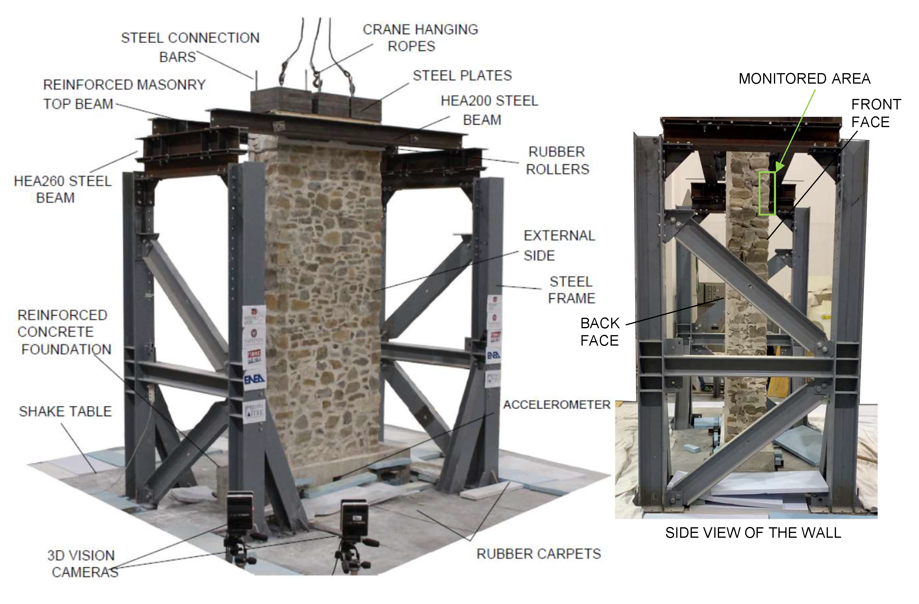
The testing setup (Figure 2 was kept identical for the three walls and was meant to mimic a vertical spanning wall fixed at the base and restrained on top by a floor connection. Aiming at releasing vertical displacements, while preventing horizontal ones, low-friction rubber rollers were placed in contrast with the top of the wall, which was reinforced with a GFRP mesh (the same used for the CRM overlay) placed in the bed joints. Rollers were supported by transverse steel beams and lateral braced steel frames [23]. The acquisition system consisted of a commercial digital camera with 24.3 megapixel resolution, placed on a tripod at approximately 4 m distance from the specimen (Figure 2, recording at a 30 fps rate.

Tests were carried out on a 4 × 4 m${}^2$, six degrees of freedom shake table, controlled by four horizontal and four vertical hydraulic actuators. The testing protocol consisted of a series of strong motion tests performed under natural accelerograms, which were recorded during the 2016–2017 sequence at Norcia (NRC), Castel Sant’Angelo sul Nera (CNE), and Amatrice (AMT) stations. Input signals were applied, with the same order as above, with increasing scale factor (SF) with 0.2 stepping. Strong motion tests were labeled using the three letters of the record station and two numbers associated with the scale factor. For instance, the test under the natural accelerogram recorded at Amatrice station multiplied by SF = 0.4 was labeled as AMT04 and each equally scaled series consisted, for example, of three subsequent signals NRC02, CNE02, AMT02, if 0.2 was the selected scale factor.

Prior to the first series of strong motion tests and at the end of each equally scaled group of tests, a white noise signal was applied by the table, with peak acceleration equal to 0.05 g, in order to let a proper dynamic identification be performed. These tests were labeled as WHT, referring to the white noise input, with a progressively increasing number (WHT01, WHT02, etc.). The application of white noise signals is instrumental in dynamic identification, as this type of excitation is more similar to that induced by real environmental inputs. It is therefore more consistent with the identification performed by recording a video with the shake table on but at rest, and allows identification of the system’s natural frequencies independently from the dominant frequencies of the input signal that could possibly lead to incorrect identification.

A high-resolution 3D motion capture system named 3DVision was used [24] to record the displacements at predetermined locations, by means of retro-reflecting spherical markers distributed on an approximately 40 × 40 cm${}^2$ grid on both sides of the wall. Additional markers were placed on the foundation, on the top beam, and on the steel structure, for a total of 38 (on the front side) + 38 (on the rear side) markers. Acquisition was performed at 200 Hz frequency by nine near-infrared digital cameras placed around the shake table.

This was the only monitoring system adopted during the tests and is used in the context of the study presented herein as the one providing benchmark frequency values, with respect to which the proposed procedure is validated, by calculating a relative error. The data obtained from 3DV acquisition, performed during either WHT and strong motion tests, were post-processed calculating the fundamental frequencies of the walls with a multi-input multi-output (MIMO) approach as follows. First, the accelerations of the four markers on the foundation were calculated by double derivation of the recorded displacements, and were considered as seismic inputs. The accelerations obtained from 48 markers on the wall, comprising between z = 1.28 m (row n. 2) to z = 3.44 m (row n. 7) and on both sides, were considered for the output (z being the height from the top of the foundation beam). Accelerations were not filtered. Then, the transfer function ($\Omega \left(f\right)$) was calculated from each input marker to each output marker and, finally, all the transfer functions were averaged. The numerous measurement points of 3DVision made it possible to average many transfer functions and derive a global dynamic characterization of the wall, minimizing the effect of possible local singularities of the response or of errors in acquired data (e.g., caused by dust or by the fall of a marker). The fundamental frequency f was determined as that corresponding to the main peak of ($\Omega \left(f\right)$). Note that the frequencies calculated with 3DVision under strong motion tests will not be considered in this study for validation and comparison with those derived from videos, because these latter ones were only recorded during WHT tests and between strong motion ones with the table at rest.

3.2. Application of the Computer-Vision-Based Method

Videos were recorded with a commercial reflex camera at 30 fps sampling rate. Given the peculiar experimental setup conditions, all the videos were recorded from the same viewpoint, conveniently chosen to capture the out-of-plane motions of the wall specimens induced by the dynamic input at the base. Videos were taken both during WHT tests and in between strong motion tests of the same series, when this was possible, i.e., with the table at rest. In this latter case, videos aimed at capturing the invisible vibrations of the structure, which were induced by the oil circulating in the pipe system (the engines of the actuators were on, even when the table was at rest). Therefore, the excitation consisted of environmental noise, closely representative of actual on-site conditions, when wind or traffic cause vibrations. These videos were labeled as ENV, referring to the environmental noise excitation, with a progressively increasing number (ENV01, ENV02, etc.). In ENV videos, no visible displacements of the wall could be detected with the naked eye and, thus, MM was considered as an essential preprocessing stage. As already mentioned, MM within a selected frequency range acts as a further signal filter, so, for consistency, WHT videos also underwent the same MM preprocessing, adopting the same frequency range and amplification factor $\alpha$. The parameters defining the MM preprocessing stage (

Table 1. Adopted parameters for motion magnification.

$\mathit{\alpha }$	${\mathit{f}}_{\mathit{min}}$–${\mathit{f}}_{\mathit{max}}$	ROI
20	2–8 Hz	20 × 10

) were kept constant for all the analyzed cases, that is, the amplification factor $\alpha$ was set to 20, the frequency band comprised between 2 and 8 Hz, and the ROI was constituted by 200 pixels (10 × 20 rectangle). It is worth highlighting that 3DVision was not able to provide results under ENV conditions, because the amplitude of marker displacements was of the same order of magnitude of the resolution of the measurement system. On the other hand, relevant information could have been derived by high-resolution accelerometers. Nevertheless, with respect to the CV-based method, this would have entailed higher cost (for purchasing sensors and acquisition system) and time effort (for setup implementation) and would have provided data in a limited number of measurement points (the locations of the accelerometers) to be established a priori.

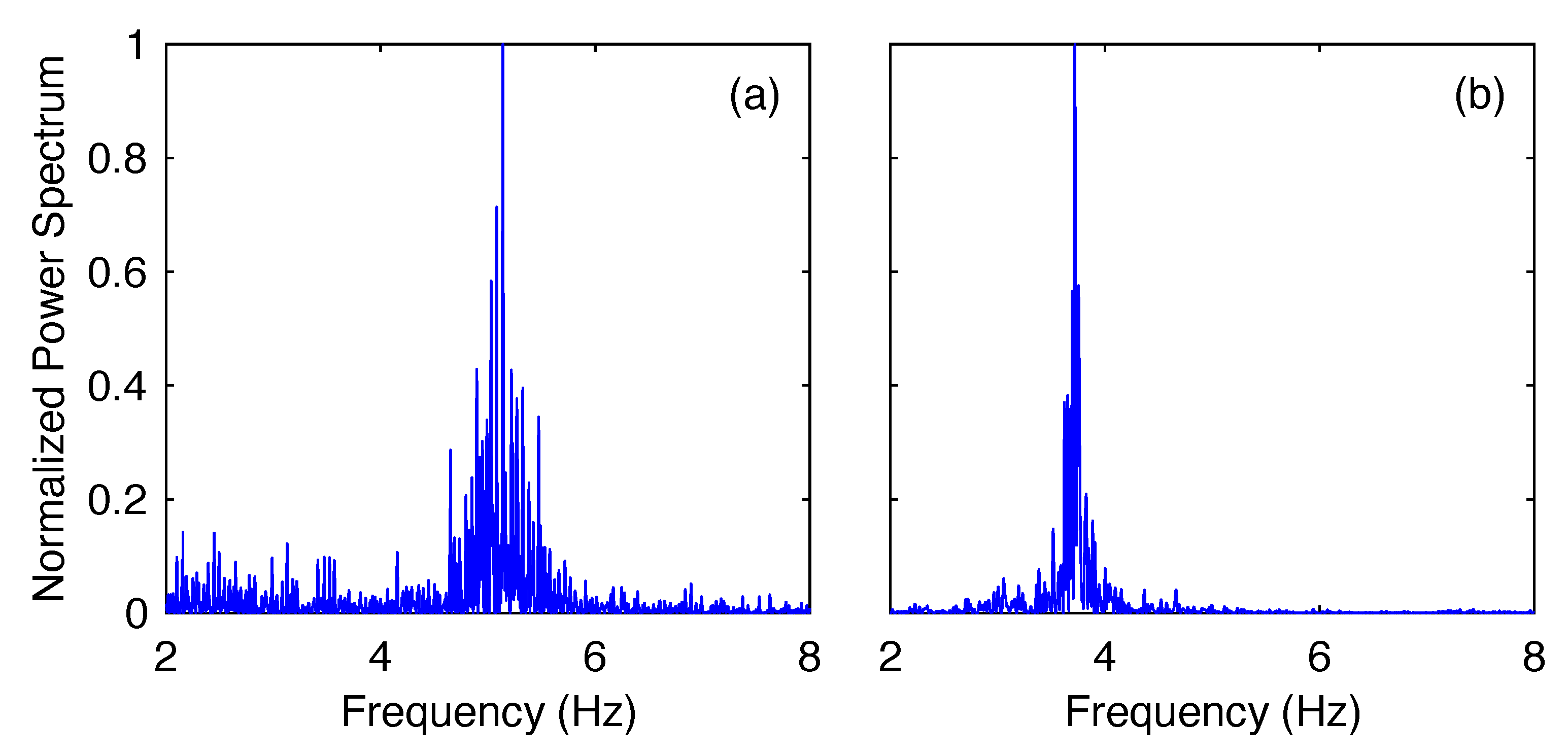
All analyses, as mentioned, were performed on a 10 × 20 region of interest; thus, 200 time histories of the pixels’ intensity variation constituted the original sample for each video. Following the flowchart reported in Figure 1, the frequency output was obtained in terms of a spectrum, from which the peak was extracted and recognized as the detected natural frequency of the wall. Figure 3 shows, as an example, the power spectra obtained for two WHT tests for UR wall (WHT01 and WHT04).

4. Results and Comparisons

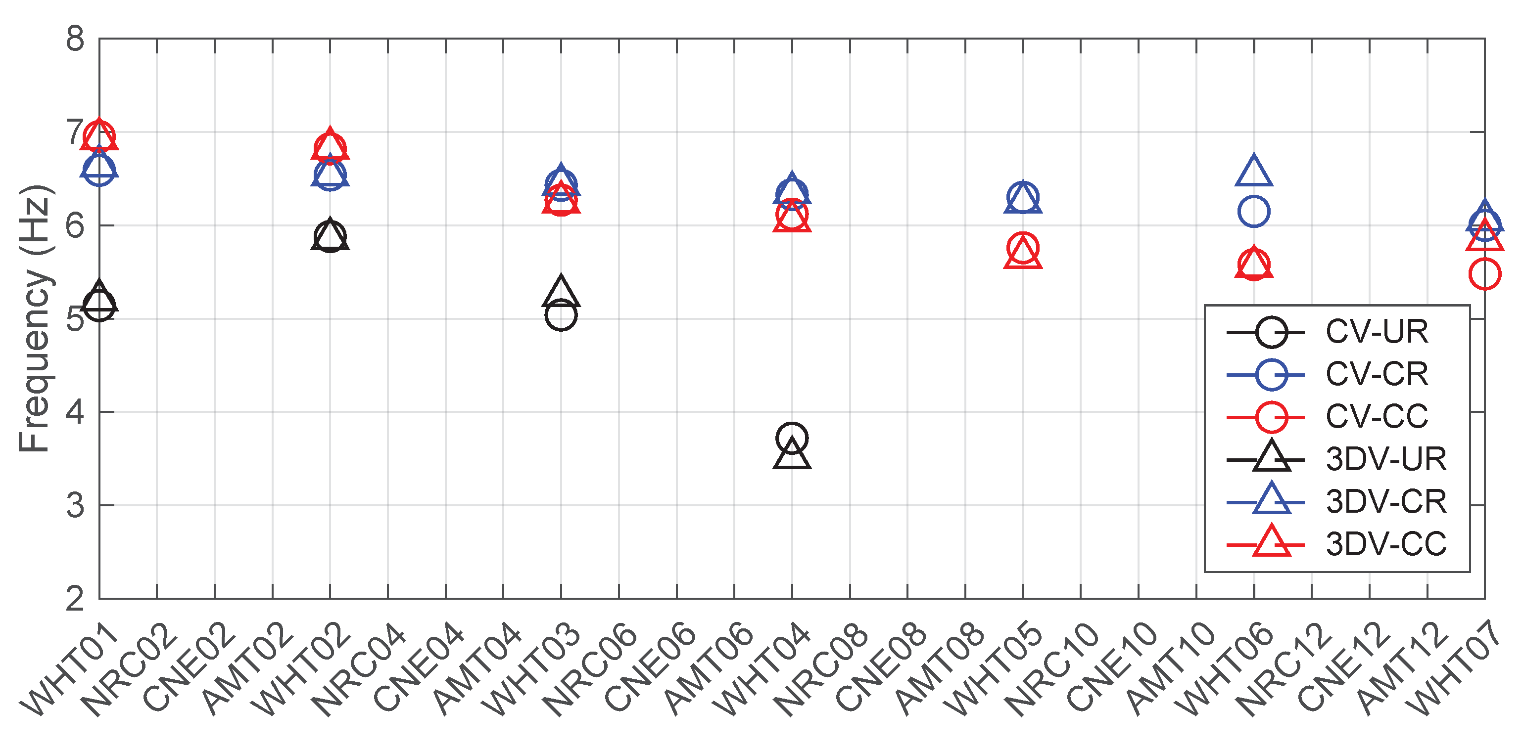
The frequencies of the three walls detected through the 3DVision (3DV) and the computer-vision-based methodology (CV) are shown in Figure 4, in which the tests are chronologically ordered on the x-axis. A direct comparison is possible only for white noise signals, as the two monitoring systems acquired data simultaneously. On the contrary, for strong motion inputs, data are available only from 3DVision, whereas for under environmental excitation, data are available only from the CV-based method. The graph shows an extremely good agreement in all cases. Both techniques detected an increase of the fundamental frequency of the UR wall between the first and the second white noise signal, which was due to a modification of the setup (the top steel beams were tightened prior to WHT02). A slightly worse performance of the CV method is envisaged in the case of the CR wall during the sixth white noise signal and for the CC wall in the case of the seventh WHT test. These discrepancies can reasonably be considered as isolated cases, related to unwanted additional vibrations induced on the camera or to an effect of the chosen ROI. Noteworthy is that this latter consists of a numerous but limited number of pixels on a predetermined portion of the wall, whereas 3DVision frequency estimates are based on an average made on markers distributed on the entire surface of the wall. The overall trend is clearly identified and, as will be more extensively discussed in the following, this will be assumed as the reference for the calculation of a damage index and the discussion of its evolution. It is noted that the trends of stiffness degradation (or, equivalently, of frequency decay) of CC and CR walls stay smooth and with an almost constant slope between one set of strong motions and the subsequent one, whereas for UR wall, the relative decrease of frequency is markedly more evident passing from WHT03 to WHT04, meaning that the series with scale factor 0.6 caused a more significant increase of damage on UR than on CC and CR, as can reasonably be expected.

The relative errors with respect to the 3DVision estimates of the fundamental frequencies for the three walls were calculated for each WHT test and are summarized in

Table 2. Adopted parameters for motion magnification.

UR	CR	CC
1.15%	0.83%	0.26%
Scale factor 0.2
0.34%	0.08%	0.10%
Scale factor 0.4
4.00%	0.14%	0.29%
Scale factor 0.6
5.98%	0.25%	1.16%
Scale factor 0.8
	0.72%	1.68%
Scale factor 1.0
	5.96%	0.36%
Scale factor 1.2
	0.99%	6.32%

. Such error is never above 6.5%, indicating that the proposed procedure is accurate in capturing the frequency of a wall subjected to white noise excitation. Nonetheless, the advantage of using this technique as an alternative to expensive accelerometers is more evident when analyzing the videos recorded between strong motion signals (ENV), when imperceptible vibrations could not be detected otherwise, as it may happen in real field conditions.

In order to provide a further representation of damage evolution, a damage index was calculated according to the following equation [25]:

$$D{I}_i=1-{\left(\frac{f_i}{f_{WHT02}}\right)}^2$$

(7)

where $D{I}_i$ is the damage index at the i-th test, $f_i$ is the detected frequency in the i-th test, and $f_{WHT02}$ is the frequency of the walls under WHT02. Conditions before WHT02 were neglected both because no significant damage occurred during strong motion tests with SF = 0.2 and because of the above-mentioned modification of the setup when the UR wall was being tested, which would have made the results not consistent. $DI$ represents damage in the 0 ÷ 1 range, such that $DI$ = 0 corresponds to no damage and $DI$ = 1 corresponds to collapse.

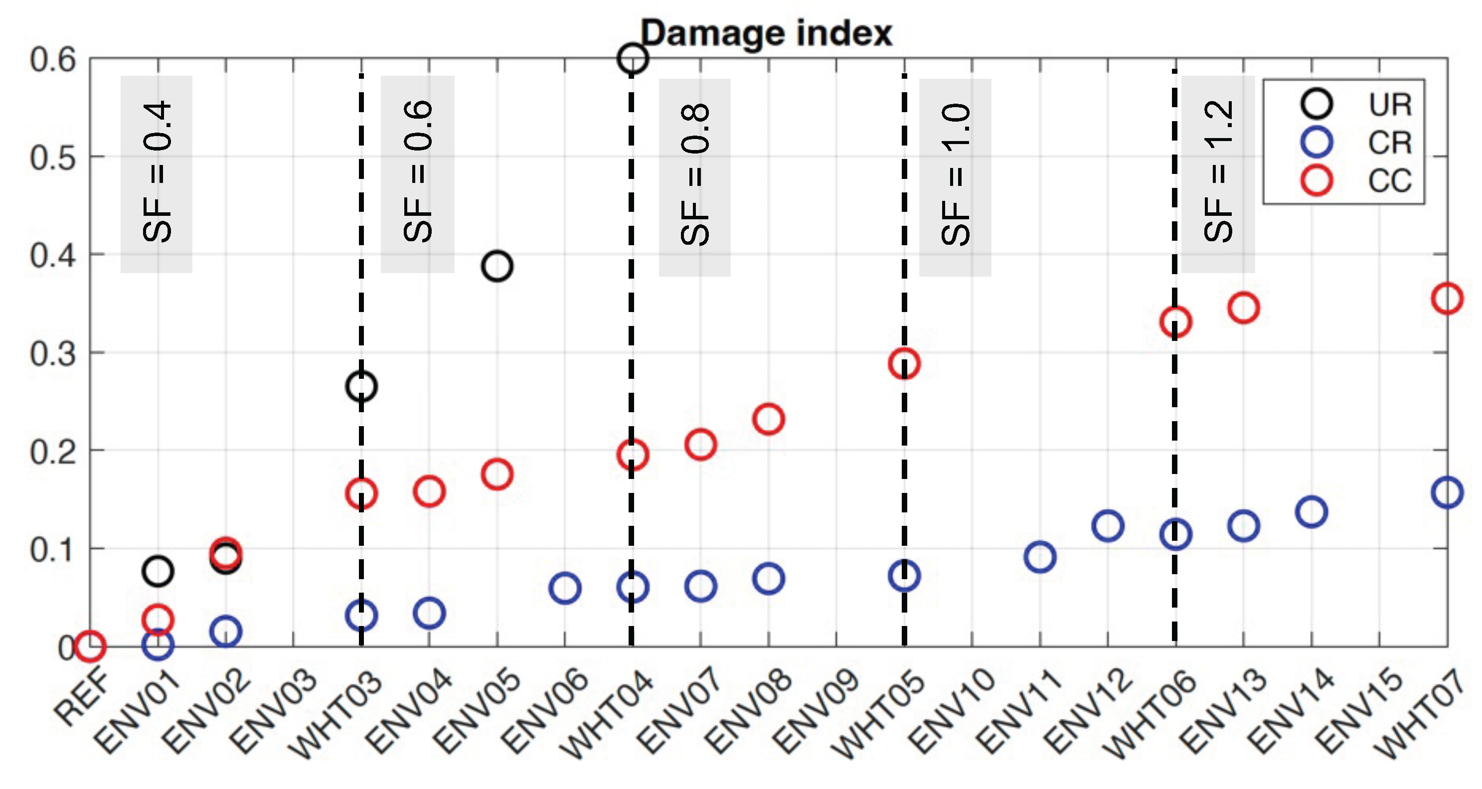
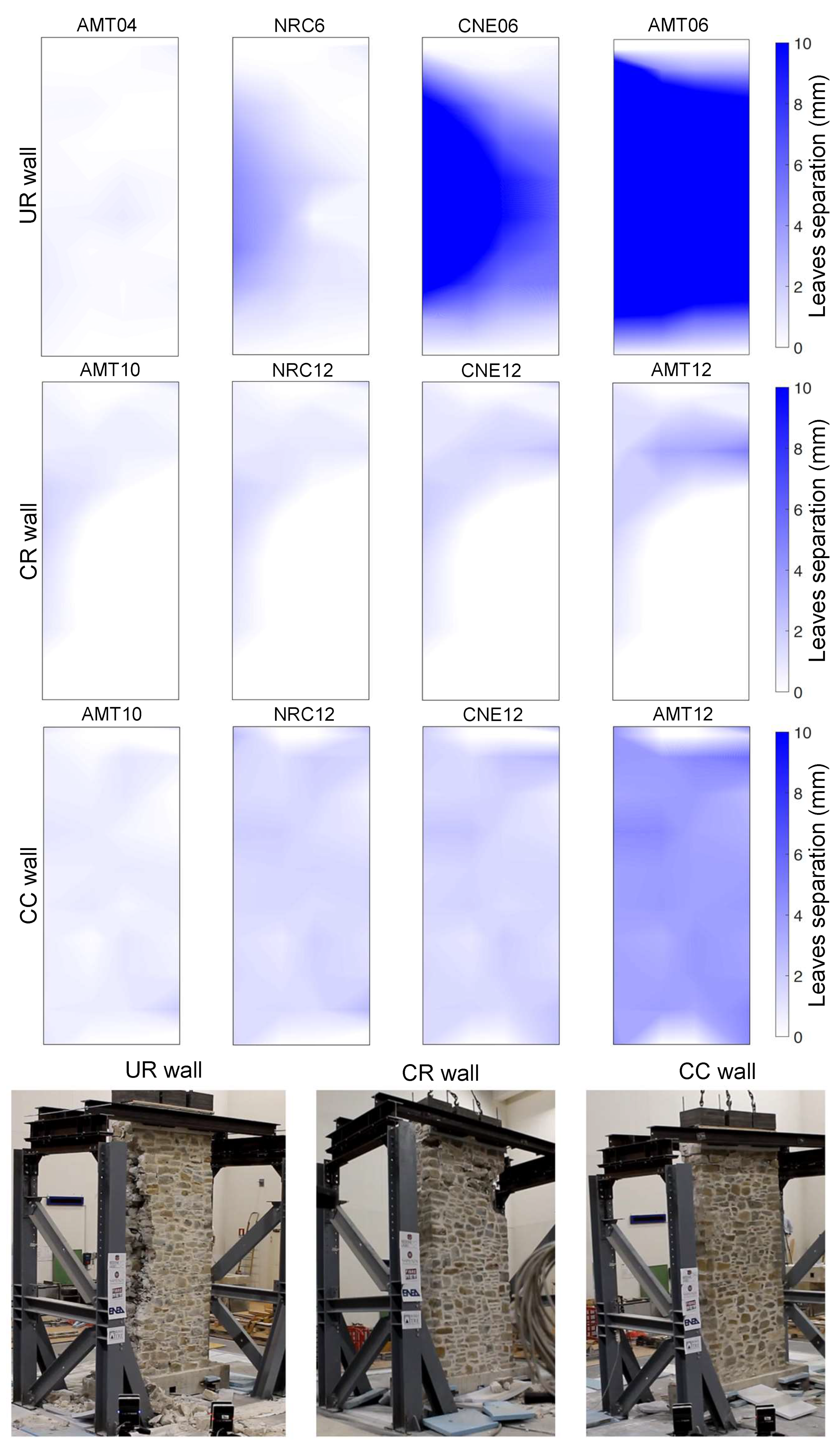
Damage index was calculated from the frequencies provided by CV either for WHT tests or for ENV video recordings. A marked nonlinear trend in plots reported in Figure 5 can be noted. Observing data referred to the UR wall, an increase in damage is first located between ENV01 and WHT03, that is, following AMT04. It is interesting to note that, during the 0.6 scaled sequence of signals, the damage increased with almost the same rate after NRC06 and CNE06, as testified by the DI value at ENV05 (immediately after CNE06). Again, the AMT signal caused a relatively higher increase of damage, highlighted by the value of DI detected for the WHT04 video, recorded during the white noise test after AMT06. Experimentally, this is confirmed looking at Figure 6, showing the progressive leaf separation measured by processing the displacements of the markers placed on the front and on the back sides of the wall. During the 0.8 scaled sequence, no further measures of DI are reported since the wall experienced the partial collapse on the monitored face (no more videos were recorded for ENV excitation), attaining a global failure under CNE08 signal.

Damage index evolution shows a different trend for CR and CC walls, which experienced less damage accumulation than UR up to the last measured point, that is, WHT07, after the 1.2 scaled sequence of strong motion tests. The slope of the DI curves seems quite constant during the experiments, whereas CC wall accumulated more damage with respect to CR, as it can also be deduced looking at the contours of leaf separation in Figure 6. For the same signal (AMT12), the last strong motion test after which videos under white noise excitation were recorded, the relative displacement between the front and the back façades shows a comparable value, but much more distributed on the whole structure in the case of the CC wall. This is reflected in the higher values attained by the DI prior to collapse, which in both cases took place during the 1.4 scaled series, resulting in the fall of stones from the upper portion of the wall. The frequency decay and the damage accumulation measured through the proposed technique result are consistent with the damage observed on the walls during the experimental investigations, as described in [21,22]. In particular, the unreinforced wall reached its ultimate limit state by exhibiting an out-of-plane bending collapse mechanism of the two wall leaves. This was accompanied by an evident crumbling phenomenon, which first affected a lateral edge of the wall and then involved the entire structure during collapse. On the other hand, in both the reinforced walls, a local failure took place. The patterns of leaves separation (shown in Figure 6) and the analyses on dynamic response and dissipated energy (reported below) highlight some differences between CR and CC. More specifically, as for the mode of failure, the wall reinforced with CRM and ultra-high-stainless-steel cord repointing (CR) showed localized failure at the top, with leaf separation and fall of stone units. The wall strengthened with CFRP connectors (CC), instead, exhibited a spread distribution of leaf separation and a limited number of stone units that fell down on the table from the portion immediately below the crowning beam (Figure 6).

During an earthquake, structures accumulate damage while dissipating energy. This can be estimated by adding up the area within all the hysteretic cycles that the system develops during the ground motion. Evaluating the dissipated energy in hysteresis cycles is recognized to be representative of the accumulation of damage in structures subjected to dynamic excitations (e.g., [26,27,28]), to which damage can be related [29,30].

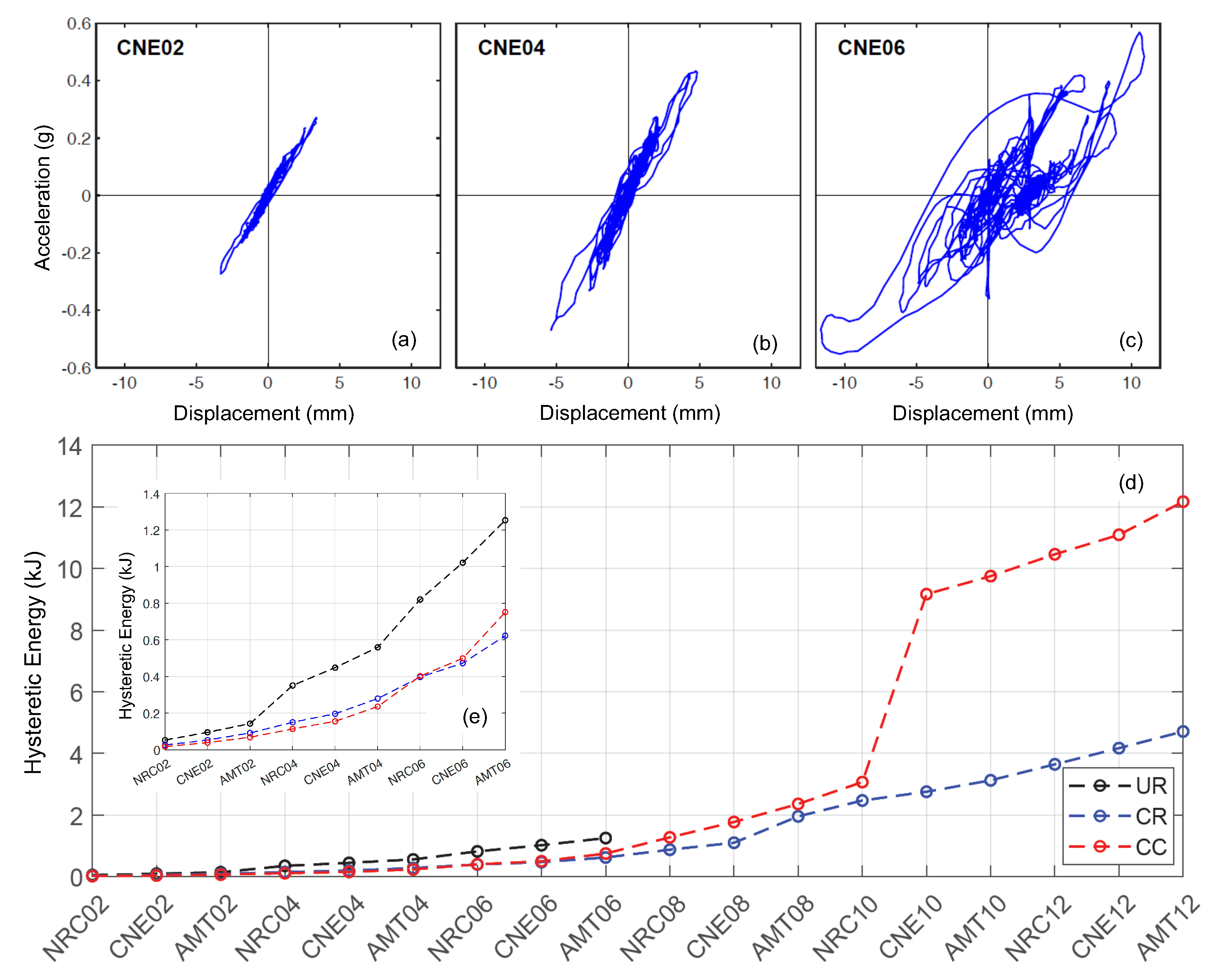
For the analyzed cases, hysteretic energy was calculated for each strong motion test by multiplying the area included in the acceleration–displacement cycles of a marker by the mass attributed to it, and then summing the contributions of all markers. Figure 7a–c show, for the sake of an example, the acceleration versus displacement cycles of one marker on the rear side of UR wall at about 2.5 m height, under three strong motion tests with the same record applied at the base (CNE), amplified by increasing SF. Figure 7d reports the cumulative hysteretic energy of the three walls under strong motion tests. On the one hand, it can be noted that the energy dissipated by CR and CC walls is sensibly higher with respect to UR, if the entire seismic sequence to which each wall was subjected is considered. This is clearly due to the much higher intensity of earthquake base motion attained by the strengthened walls with respect to the unstrengthened one. On the other hand, focusing on the first series of signals (up to AMT06) reported in Figure 7e, it is evident how the cumulative dissipated energy is markedly higher for UR than for CC and CR. This indicates that, under the (nominally) same base inputs, UR wall experienced a heaver damage, which is consistent with both the experimental evidences (crack pattern and progressive damage evolution) and with the damage index trend reported above. Both the frequency decay and the damage index exhibit an almost linear trend. On the other hand, the evolution of cumulative dissipated energy is markedly nonlinear, due to the higher base accelerations achieved at collapse. The higher dissipated energy estimated for CC wall with respect to CR wall was attributed to the wider area interested by leaves separation.

5. Conclusions

A computer-vision-based structural health monitoring methodology was applied to determine the natural frequency of three rubble stone masonry walls tested on the shake table and to track the progressive damage accumulation correlated with the frequency decay occurring along the experimental investigation. Videos were recorded with commercial cameras at standard acquisition frequencies, both under white noise excitations produced by the shake table and under environmental vibrations, with the table at rest, closely representative of actual on-site conditions under the effect of wind or traffic. The small amplitude of recorded oscillations in this latter case made it necessary to preprocess videos with motion magnification algorithms.

Frequencies under white noise excitation were compared to those measured by a high-resolution passive 3D motion capture system, named 3DVision, installed at the shake table laboratory, revealing an extremely good agreement. The results of the CV-based method under environmental vibrations, which could not be even obtained by 3DVision, well captured the progressive frequency decay, consistently with the evolution of damage observed experimentally and detected by 3DVision under strong motion earthquake inputs.

On the basis of the frequency decay, a damage index was calculated, whose evolution was judged compatible with the trend of the hysteretic energy obtained from 3DVision measurement and with phenomenological evidence surveyed in the laboratory during test execution and by data related to leaf separation.

Despite that the validation of the CV-based structural health monitoring methodology described in this paper was performed under controlled laboratory conditions, the outcomes of this study clearly indicate the great potential of the method and set the stage for more complex and real on-site applications on full-scale structures under environmental actions. In this context, based on the experience gained in the laboratory, the combination of the proposed procedure with motion magnification algorithms will undoubtedly represent an essential and unavoidable preprocessing step. Ongoing research on this topic is being devoted to the analysis of case studies in real environments, to validate the procedure and to highlight issues related to ambient conditions and real field excitations on large-scale structures. Compared to other dynamic identification strategies, the relatively cheap equipment and the limited computation time required by the proposed approach make it an appealing alternative. Nevertheless, it still needs to be validated on a wider database of case studies before it can be routinely adopted in the engineering practice.