Abstract
With rapid urbanisation in China, sustainable urban development faces a major obstacle due to insufficient consideration of land-use efficiency. Currently, despite progress in analysing land-use efficiency, not every land manager has enough knowledge of green land use from a county perspective. Therefore, the objective of this research is to explore the spatiotemporal evolution law focused on county green land-use efficiency (CGLUE), which can support sustainable county development. Based on 10 specific CGLUE factors identified through a content-mining tool, this study explored the temporal and spatial evolution law of 11 counties in Sichuan Province using the ultra-efficient slacks-based measure (SBM), kernel density estimation, and Moran’s I statistic. The study found that (1) CGLUE factors cover the administrative area, total investment in fixed assets by region, the number of employed persons in secondary and tertiary industries, gross domestic product in secondary and tertiary industries, the average wage of staff and workers, basic statistics on per capita park green area, carbon emissions of land, the volume of industrial wastewater discharged, the volume of industrial sulphur dioxide emission, and the volume of industrial soot (dust) emission; (2) from a time-evolution perspective, CGLUE shows an increasing trend of time series evolution as a whole, and its dynamic evolution process has obvious differences in time. CGLUE increased, and the difference in CGLUE became larger from 2010 to 2012. CGLUE also increased, and the difference in CGLUE became smaller from 2013 to 2016. CGLUE also increased, and the difference in CGLUE became larger from 2017 to 2020; (3) from a spatial evolution perspective, the global spatial evolution laws of CGLUE show that the spatial agglomeration state has gone from strong to weak. Overall, however, Sichuan Province CGLUE maintains a high spatial agglomeration effect. The local spatial evolution laws show that the CGLUE of the 11 counties is positively correlated. The high–low CGLUE agglomeration areas are mainly distributed in Chengdu, Mianyang, Meishan and Yibin; the low–low CGLUE agglomeration areas are mainly distributed in Deyang, Yaan, and Zigong. The novelty of the research lies in these aspects: (1) the carbon emissions of land should be considered the undesired output of CGLUE; (2) CGLUE in Sichuan Province has various growing stages from a time perspective; (3) CGLUE in Sichuan Province has a high spatial concentration in Chengdu from spatial view, and these counties’ resources flow and interact at high speed. These findings offer a solid reference for the sustainable development of these 11 counties in Sichuan Province.
1. Introduction
The complex characteristics of rapid urbanisation can make urban land use irrational and inefficient, decreasing arable land and causing disorderly urban sprawl, less green space, and a heat island effect [1,2]. Therefore, it is critical to have harmony between population growth and urban development [3,4]. The key to sustainable urban development is to realise efficient urban land use [5]. Efficient urban land use can improve land value even when land supply is limited, and it is necessary for sound environmental and economic growth.
Efficiency refers to the most efficient use of resources under given conditions to meet set needs and visions. Urban land-use efficiency refers to the many economic benefits and pollutants that can be generated per unit of urban land area. In the context of economic globalisation, urban land-use efficiency is associated with economic structures, industry input, land use, and urban planning [6,7]. Urban land-use efficiency contains factors such as the scale of the primary industry, the scale of the secondary industry, the scale of the tertiary industry, urban area, waste discharge, and urban population [8,9,10]. Previous studies have explored a series of factors measuring urban land-use efficiency [11], but they have rarely given enough attention to the integration of green and low-carbon elements into urban land-use systems. Therefore, this study aims to explore land-use efficiency by considering green and low-carbon elements.
County green land-use efficiency (CGLUE) refers to using the lowest land-use cost to generate maximum benefits to improve an area’s economy, environment, and quality of life for the residents [12,13]. Compared with urban land-use efficiency, CGLUE pays more attention to low-carbon elements. These refer to, under the conditions of the county, limited land area, reasonable industrial layout, and development methods that help counties produce high economic benefits, better ecological environments, and low-carbon emissions. Some previous studies have researched the evaluation systems, spatial patterns, and regional differences in land-use efficiency in big cities [14,15,16]. However, these studies of revolving land-use efficiency have not paid attention to the practically sustainable development requirements of a county [17]. It is difficult to mitigate illegal county land use, environmental pollution, and economic downturn. Table 1 lists a total of 80 county unsustainable development accidents in Sichuan Province issued by official reports from 2009 to 2022. The root cause of inefficient land use is illegal land grants by county management committees, accounting for 35%, which reflects that county managers cannot understand the temporal and spatial evolution laws of CGLUE. Therefore, to avoid disorder in land approvals, it is necessary to recognise specific factors and understand the status of CGLUE.

Table 1.
Unsustainable county development accidents.
This research analysed this issue by focusing on four questions: (1) Which factors can measure CGLUE? (2) How does the law of CGLUE operate in different counties under time series? (3) How do the global evolution law of CGLUE and the local agglomeration effect of CGLUE operate in different counties under spatial series? The findings of this research will not only contribute to the literature on CGLUE assessment and add knowledge to county land resources management, but it will also offer some suggestions to county managers.
2. Literature Review
It is widely accepted in the literature that efficient land use in urbanisation plays a critical role in improving sustainable urban development [18]. Efficient land-use strategies should reconcile economic, environmental, and social sustainability [19]. Recently, many urban land-use efficiency studies have been presented that, for example, recognise the characteristics of land-use efficiency and metropolitan agglomeration [20,21].
Concerning urban land-use efficiency, some studies have pointed out that rapid urbanisation has caused serious environmental pollution, and urban land-use efficiency should consider the environment, social sustainability, and governance [22,23,24]. Many studies verify that urban land-use efficiency has three aspects: economic level, industry structure, and government regulation. These aspects often cover per capita gross domestic product (GDP), population density, and the degree of market openness [25,26,27]. Some studies used system information modelling (SIM) to verify that land-use efficiency can be measured by three aspects: innovation, industrial structure, and economic connections. It has been pointed out that technological processes, pure technical efficiency, and scale efficiency are the main aspects of urban land-use efficiency [28,29]. Industrial structure and population density affect environmental regulations, and these regulations affect urban land-use efficiency [30,31].
Various factors of urban land-use efficiency stem from environmental, social, and governance elements. A study by [32] used 26 cities in the Yangtze River delta as an example to build an evaluation system for urban land-use efficiency under the green development concept, which contains the inputs of land, capital, labour, and energy factors in the process of urban development. Ref. [33] used the super-efficiency slacks-based model (SBM) of data envelopment analysis (DEA) and partial least squares structural equation modelling to analyse the data of 35 cities to measure urban land-use efficiency and explore the key driving factors. Their study pointed out that urban land-use efficiency is related to the spatial heterogeneity of different regions, and the efficiency had a 0.17% rise from 2007 to 2015. It was noted that land-use efficiency contained economic, infrastructure, and market elements.
Many studies have paid much attention to assessing urban land-use efficiency in different years. For example, the human appropriation of the net primary production (HANPP) framework has been used to analyse land-use efficiency in New Zealand. One study found that efficiency increased from 1860 to 1920, declined in 1950, increased to 41% in 1980, and declined to 32% in 2005 [34]. The Malmquist index approach was used to measure and decompose urban land-use total factor productivity, and a pane vector autoregressive model was used to investigate the interactions among urban land-use total factor productivity, technological progress, pure technical efficiency, and scale efficiency in China from 2003 to 2016 [29]. That study showed that overall urban-land use efficiency increased at an annual growth rate of 0.7%. Some scholars measured green land utilisation efficiency in the Beijing–Tianjin–Hebei urban agglomeration from 2006 to 2016 and found that efficiency in 2016 was higher than in 2006, and energy and environment were the driving factors affecting green land use [35]. The study also found that the efficiency of each city was positively correlated with its economic development and negatively correlated with construction land expansion.
Different cities have different urban land-use efficiency. Europe and Japan have the lowest population growth rate and land consumption rate, which indicates that these regions have high urbanisation, and more attention should be paid to the coordination of urban land use and population growth in cities [36]. Meanwhile, wealthy cities have higher urban land-use efficiency compared with poor cities, indicating that urban land-use efficiency is associated with per capita disposable income. For example, Western, Atlantic, and Central Europe have high land-use efficiency, according to the results of a comparative analysis of 417 metropolitan regions in Europe [19]. Urban land-use efficiency varies significantly across the country, and the mean efficiency values in the eastern, central, and western regions are 0.733, 0.535, and 0.507, respectively [37]. The spatial regression model was used by [30] to analyse the spatial effects of urban land-use efficiency. Their study pointed out that urban land-use efficiency was sensitive to regional heterogeneity and city size. Moreover, ref. [38] found that Xi’an had inefficient urban land use. Their study showed that land-use efficiency in the old urban area and the mature built-up area was relatively high, and the land-use efficiency of the emerging expansion area and the edge area was relatively low. ArcGIS was used to assess spatiotemporal land-use changes between 2007 and 2019. The findings revealed a prevalence of urban land-use inefficiencies in all cities in Ethiopia, the rate of land consumption in most cities far exceeded the population growth rate, and densification (urban infill) was low and slow [39].
Overall, this study is interested in urban land-use efficiency. It recognises relevant factors and evaluates many urban land-use efficiencies. However, previous studies have paid little attention to county land-use efficiency and have ignored the carbon emissions of land use. Therefore, the key issue of the study is exploring the temporal and spatial evolution law of county green land-use efficiency. Section 3 outlines the research methods, Section 4 details the reasons for choosing Sichuan Province and the data analysis methods, and Section 5 illustrates the results. Discussion of the findings follows in Section 6, conclusions are drawn in Section 7, and limitations and future research directions are outlined in Section 8.
3. Research Methods
This study’s analysis of the spatiotemporal evolution characteristics of CGLUE in the study areas involved four steps. Firstly, a content-mining tool was used to recognise the CGLUE factors. Secondly, relevant data were analysed by SBM to calculate CGLUE in the study areas. Thirdly, the kernel density estimation was used to reveal the time-series dynamic evolution law of CGLUE. In this third step, each CGLUE corresponded to a kernel density value. Kernel density estimation can convert the discrete CGLUE of each county into a continuous function curve, which is convenient for seeing the trend of the CGLUE in each county over time. Rather than using discrete points that were not always legible, this study analysed the CGLUE time evolution law based on the continuous function curve. Fourth, Moran’s I statistic was used to reveal the spatial dynamic evolution law of CGLUE. In this fourth step, the global Moran’s I statistic analysed the overall change in the spatial agglomeration state in the study areas. The local Moran’s I statistic analysed the agglomeration of CGLUE in each county from the spatial perspective. Detailed information about the research steps is presented in Figure 1.
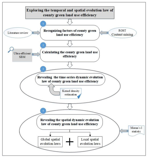
Figure 1.
The general framework of this research.
3.1. Content Mining
ROST CM6.0 (ROST content-mining system version 6.0) is a word-segmentation system software used in content analysis. The advantage of ROST content mining is that it can directly and simultaneously segment words, merge synonyms, delete nonsensical words, and search online for critical words from the literature and reports [40,41]. Another advantage of ROST CM6.0 is that it can acquire assessment information by objective and qualitative data, reducing the subjectivity of research results. Detailed information on the basic operation principles of ROST is given in Figure 2.
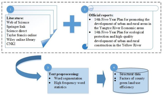
Figure 2.
Basic operation principles of ROST content mining.
3.2. Ultra-Efficient SBM
First proposed by Charns in 1978, DEA (data envelopment analysis) is an efficient method for evaluating decision-making units with multiple input and output indicators [42,43]. DEA methods mainly use the CCR (Charnes Cooper and Rhodes), the BCC (Banker, Charnes and Cooper), and the SBM models [44,45]. The CCR model is used to measure the total efficiency of decision-making units (DMU) in the case of fixed returns to scale. The BCC model is used to measure the pure technology and scale efficiency of DMU under dynamic returns to scale. The CCR and BCC models usually take the radial measurement as the premise, assuming that the input and output change is in the same proportion, although few such situations exist. Compared to these models, the SBM model can effectively avoid these shortages. The advantage of the ultra-efficient SBM is that it can eliminate the deviation and influence caused by the difference between the radial and angular selection and reflects the slack variables of surplus input and insufficient output [46,47]. Another advantage of the ultra-efficient SBM is that it can evaluate decision-making units whose efficiency value is greater than 1, obtaining more accurate efficiency results [48]. Therefore, this study used the ultra-efficient SBM to explore the CGLUE in the study areas. The detailed calculation equations are given below:
In Equation (1), represents the CGLUE index; is the number of DMU; is the number of input elements; is the expected output; is the undesired output. Vectors , , and are input vector, expected output vector, and undesired output vector, respectively. Matrix , , . , , and are the input slack variable, the expected output slack variable, and the undesired output slack variable, respectively; is the weight vector.
In the above equations, when the CGLUE index is ≥ 1, the decision-making unit is effective, and the CGLUE is effective. When the CGLUE index is 0 ≤ < 1, the decision-making unit may be ineffective, and the CGLUE is relatively low. The county needs to further improve the ratio of input and output to achieve the best efficiency.
3.3. Kernel Density Estimation
The kernel density estimation is a nonparametric method used to estimate the dynamic distribution characteristics of data based on the time perspective [49,50]. The advantage of the kernel density estimation is that it can avoid the subjectivity of function settings when estimating the parameter and improve the accuracy of estimation results [51,52]. Another advantage of the kernel density estimation is that it can accurately calculate the average effect of all sample points from a time perspective [53,54]. Therefore, this study conducted kernel density estimation to reveal the time-series dynamic evolution law of CGLUE. The detailed equation is presented below:
In Equation (2), represents the number of samples; represents the window width;; is a kernel function; denotes the ith sample. The kernel functions contain several types, including the uniform kernel, the Gauss kernel, the Epanechnikov kernel, and the quadric kernel. The different kernel functions have little impact on the results. This study used the uniform kernel to conduct the kernel density estimation. It uses uniform kernel density to convert the discrete CGLUE of each county into a continuous function curve, which is convenient for analysing CGLUE time evolution law.
3.4. Exploratory Spatial Data Analysis
Exploratory spatial data analysis (ESDA) is a series of techniques and methods mainly used to reveal spatial distribution law and the spatial interaction mechanism of data. Moran’s I statistic is an effective ESDA method that measures global spatial autocorrelation and the local spatial agglomeration effect [55,56]. The advantage of the Moran’s I statistic is that it can be combined with maps to test spatial independence, and map results are visual and intuitive for easy decision-making [57]. Another advantage of the Moran’s I statistic is that it can analyse objective data to alleviate the uncertainty of subjective data. Recently, Moran’s I statistic has been used in real estate, urban management, public health, and disease mapping [58]. In this study, research was aimed at finding the different counties’ autocorrelation in CGLUE and the spatial agglomeration effect of CGLUE, which needed a mapping result. Therefore, Moran’s I statistic was selected to analyse the spatial evolution law of CGLUE. The basic calculation rules of the global Moran’s I statistic are represented in Equation (3), and the local Moran’s I statistic calculation steps are presented in Equation (4):
In Equations (3) and (4), Moran’s I is the Global Moran’s I statistic, and is the local Moran’s I statistic. is a distance weight between and , which can be specified as a distance band [59]; and are green county land-use efficiency in county and j county; represents the mean of the CGLUE of all counties; is the number of observations. and are the normalised values of CGLUE for i county and j county, respectively.
Moran’s I statistic distribution range is [−1, 1]. When the distribution range is [0, 1], there is a positive correlation between the efficiency values of each geographic entity. When the distribution range is [−1, 0], there is a negative correlation between the efficiency values of each geographic entity. A value of 0 represents no correlation between the efficiency values of each geographic entity.
4. Data Collection and Analysis
4.1. Study Area
The study area of this research comprises 11 counties located in Sichuan Province, and the boundaries of Sichuan province on the map of China have been marked in green, represented in Figure 3. The counties are Chengdu, Zigong, Panzhihua, Luzhou, Deyang, Mianyang, Suining, Guangyuan, Meishan, Yibin, and Yaan (see Figure 4, where the areas are marked in purple on the map).
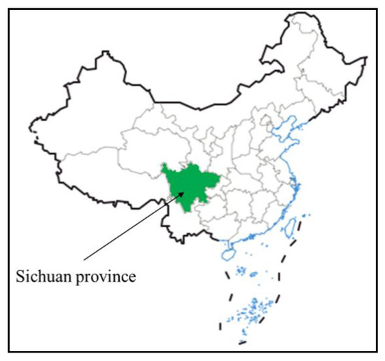
Figure 3.
Boundaries of Sichuan province in China.
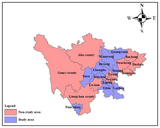
Figure 4.
The 11 counties of Sichuan Province selected for this research.
There were two reasons for choosing Sichuan Province. First, China has recently begun paying more attention to interior urban economic development, and Sichuan Province has a prominent position in China’s interior. China regards the development of Sichuan and Chongqing as national development goals, where urbanisation has an important role to play in analysing China’s urban development. Second, Sichuan Province attaches great importance to the coordinated development of environmental protection, economic development, and social harmony, providing a good foundation for this research on CGLUE.
The 11 counties were chosen for two reasons. First, they have relatively fast economic development, high intensity of land development, and high-speed operation of resource input and output. As the key counties in Sichuan Province, they represent the overall CGLUE of the province to a certain extent. Second, regarding the availability of data, these 11 counties have complete data, while other counties have incomplete data. The complete data can calculate the most real Moran statistics and fully present the spatiotemporal distribution law of CGLUE.
4.2. Data Collection
First, in the process of recognising the CGLUE factors, literature-based data were mainly collected from public sources found through:
- The Chinese Social Sciences Citation Index and the Chinese Science Citation Database journal articles in China National Knowledge Infrastructure (CNKI);
- Science Citation Index Expanded and Social Sciences Citation Index journal articles in Web of Science Core Collection;
- Other high-quality studies from SpringerLink, ScienceDirect, Taylor & Francis Online, and Wiley Online Library;
- The targets of the “14th Five-Year Plan for promoting the development of urban and rural areas in the Yangtze River Economic areas” and the “14th Five-Year Plan for ecological protection and high-quality development of urban and rural construction in the Yellow River” issued by the Ministry of Housing and Urban–Rural Development of China.
Second, in calculating CGLUE, data were collected from official reports and websites. This study selected the panel data of 11 counties in Sichuan Province from 2010 to 2020 as the research samples. The data came from the Sichuan Statistical Yearbook (2010–2020), the Chengdu Statistical Yearbook (2010–2020), the Sichuan Provincial Bureau of Statistics, and the China National Statistical Database. In particular, carbon emissions were calculated by the weighted sum of various energy consumptions, the coefficient value of converted standard coal, and the carbon emission coefficient. These energy sources contain raw coal, coke, petroleum pitch, petroleum coke, gasoline, kerosene, diesel, fuel oil, liquefied petroleum gas, natural gas, and electricity.
4.3. Data Analysis Tools
First, to recognise the GGLUE factors, the researchers reviewed all critical studies. The factor-recognition process was divided into two steps: (1) the most frequent factors were recognised by the ROST content-mining tool according to the number of occurrences of each factor; (2) these factors were then divided into several categories based on the principle of attribute similarity.
Second, to calculate the CGLUE from 2010 to 2020, according to the theory of ultra-efficient SBM, the CGLUE data were analysed by MaxDEA software.
Third, the CGLUE time evolution law was analysed by Stata 16 software. The software analysed the time evolution law of the green land-use efficiency of the 11 counties from 2010 to 2020.
Fourth, to analyse the CGLUE spatial evolution law, this study employed GeoDa software to explore global and local spatial evolution laws in the study areas.
5. Research Findings
5.1. CGLUE Factors
As shown in Table 2, the CGLUE factors were recognised. They contain five parts involving land resources, capital resources, labour resources, expected output, and undesired output. The ROST content-mining software recognises 252 records related to CGLUE, including 23 high-frequency words, 10 of which have more than 60 frequencies. According to the principle of the minority obeying the majority, words with more than 60 frequencies often appear in related texts, and they can measure CGLUE. Therefore, this study has regarded these 10 high-frequency words as the CGLUE factors. Detailed information on the CGLUE factors can be found in Table 2. The findings in Table 2 are highly consistent with reality, where the Ministry of Ecology and Environment of the People’s Republic of China often measure urban pollutant emissions by the volume of industrial wastewater discharged, the volume of industrial sulphur dioxide emission, and the volume of industrial soot (dust) emission. The National Development and Reform Commission in China often uses total investment in fixed assets by region and the number of employed persons in secondary and tertiary industries to measure the resource input of urban development.
Table 2.
Factors of CGLUE.
According to data-collection rules, detailed information on CGLUE factors values is represented in the Supplementary File.
5.2. CGLUE Results
This study indicates that county green land-use efficiency can be perfect sometimes, while inefficient at other times, as shown in Figure 5 and Figure 6. Detailed information on the 11 counties’ CGLUE from 2010 to 2020 is given in the Supplementary File. The most efficient counties are Chengdu, Panzhihua, and Zigong. The top five efficient counties are Panzhihua in 2012 (ρ = 3.399), Zigong in 2017 (ρ = 2.649), Zigong in 2018 (ρ = 2.535), Chengdu in 2018 (ρ = 2.433), and Panzhihua in 2011 (ρ = 2.226). The most inefficient counties are Luzhou, Mianyang, and Yibin. Detailed information is shown in Figure 7. The efficient counties are marked in red, and the inefficient counties are marked in yellow. In Figure 7, the counties with moderate efficiency are marked in blue, and grey areas are not analysed.
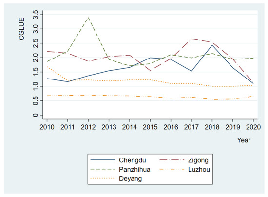
Figure 5.
CGLUE results in Chengdu, Zigong, Panzhihua, Luzhou, and Deyang.
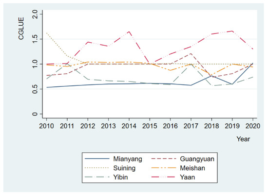
Figure 6.
CGLUE results in Mianyang, Guangyuan, Suining, Meishan, Yibin, and Yaan.
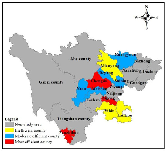
Figure 7.
CGLUE in 11 counties of Sichuan Province.
5.3. Results of CGLUE Time-Evolution Laws
In terms of the time-series perspective of these 11 counties, Figure 8, Figure 9 and Figure 10 show their time-evolution features. In these figures, the x-axis represents the comprehensive CGLUE value of the 11 counties, and the y-axis represents the comprehensive kernel density value of the 11 counties. The distribution location, shape, and polarisation phenomenon of the curve trend reveal the time-series dynamic evolution law of 11 countries’ CGLUE from 2010 to 2020. This study explored several time-evolution laws of CGLUE in the following.
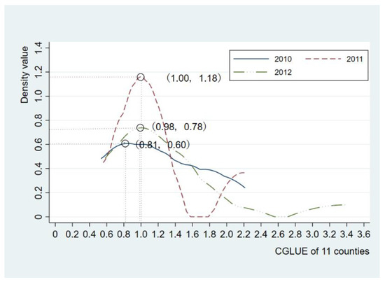
Figure 8.
Efficiency kernel density curve from 2010 to 2012.
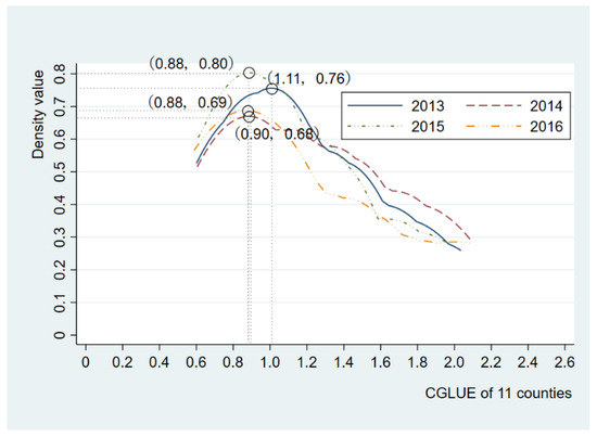
Figure 9.
Efficiency kernel density curve from 2013 to 2016.
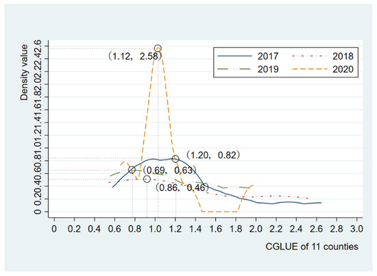
Figure 10.
Efficiency kernel density curve from 2017 to 2020.
First, the central axis of the curve is slowly shifting to the right overall. The central axis interval from 2010 to 2020 are 0.81, 1.00, 0.98, 1.11, 0.90, 0.88, 0.88, 1.20, 0.86, 0.69, and 1.12, respectively. This shows that although the efficiency of these 11 counties fluctuates in these years, the fluctuation range is not large, and it fluctuates around 1. It also shows that the CGLUE in Sichuan is fluctuating, but the overall level is growing.
Second, it further develops the perspective of the shape of the nuclear density curve. Figure 8 shows that the nuclear density curves in 2011 and 2012 have two double peaks, and 2010 is a single peak. This indicates that there was a discrete phenomenon in CGLUE in 2011 and 2012, the difference in CGLUE between counties gradually increased, and there was a slight polarisation phenomenon in 2011 and 2012. Figure 9 shows that each of the four curves has only one peak. This indicates that the CGLUE in 2013, 2014, 2015, and 2016 increased and converged, and the differences between counties gradually narrowed. Figure 10 shows that the nuclear density curves in 2017, 2018, and 2019 have a different single peak, and 2020 has a double peak. This indicates that there was a converged phenomenon in CGLUE from 2017 to 2019; the difference in CGLUE between counties gradually narrowed. In 2020, there was a discrete phenomenon in CGLUE, the difference in CGLUE between counties gradually increased, and there was a significant polarisation phenomenon in 2020.
Therefore, CGLUE shows an increasing trend of time-series evolution as a whole, and its dynamic evolution process has obvious differences in time. From 2010 to 2020, CGLUE went through three stages: (1) a single peak evolved into a double peak from 2010 to 2012, (2) a different single peak evolved into a different single peak from 2013 to 2016, and (3) a different single peak evolved into a different double peak from 2017 to 2020. Meanwhile, the central axis of the curve slowly fluctuated and shifted to the right overall. The above features indicate that in stage (1), CGLUE increased, and the difference in CGLUE became larger from 2010 to 2012. In stage (2), CGLUE also increased, and the difference in CGLUE became smaller from 2013 to 2016. In stage (3), CGLUE also increased, and the difference in CGLUE became larger from 2017 to 2020.
5.4. Spatial Evolution Laws of CGLUE
5.4.1. Global Spatial Evolution Laws of CGLUE
Table 3 reflects the global Moran’s I statistic of CGLUE in the 11 counties. The global Moran’s I statistic is both positive and significant at the 0.05 level. This indicates that the CGLUE in the 11 counties is positive spatial aggregation. In addition, from 2010 to 2020, the global Moran’s I statistic first increased and then decreased. The global Moran’s I statistic continued to increase from 2010 to 2019, and the spatial aggregation of CGLUE continued to increase. In 2020, the global Moran’s I statistic of CGLUE decreased to 0.428. This reflects a change in the spatial agglomeration state from strong to weak and indicates that the differences in CGLUE expanded. Overall, the degree of spatial agglomeration from 2010 to 2020 is presented in Figure 11. This scatterplot shows that CGLUE fluctuates between 0.3 and 0.6. This indicates that the spatial aggregation of the CGLUE of the 11 counties remained higher.
Table 3.
Global Moran’s I statistic of CGLUE in study areas.
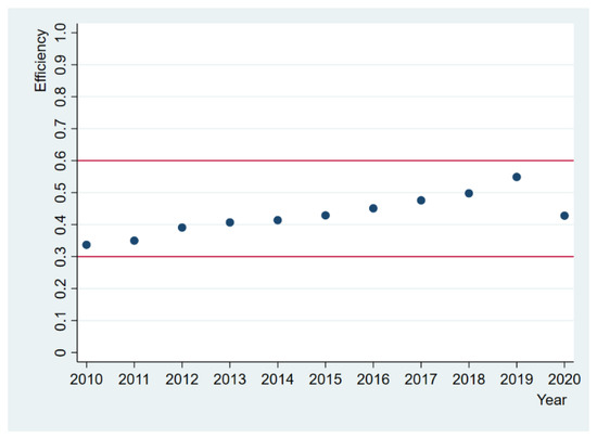
Figure 11.
The degree of spatial agglomeration of CGLUE.
5.4.2. Local Spatial Evolution Laws of CGLUE
These results of the local spatial evolution laws are dynamic, the high–low CGLUE agglomeration areas are increasing, and many resources of Sichuan province are gathered in Chengdu. For example, Figure 12, Figure 13 and Figure 14 reflect the LISA aggregation diagram of CGLUE in the 11 counties in 2010, 2015, and 2020, respectively. They indicate that the CGLUE of the 11 counties presents the characteristics of different high–low adjacency and low–low adjacency.
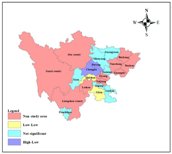
Figure 12.
LISA aggregation diagram of the 11 counties’ CGLUE in 2010.
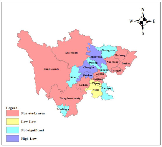
Figure 13.
LISA aggregation diagram of the 11 counties’ CGLUE in 2015.
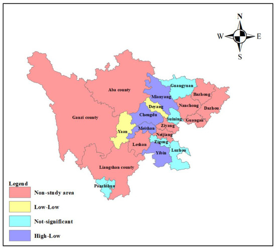
Figure 14.
LISA aggregation diagram of the 11 counties’ CGLUE in 2020.
In these figures, the purple areas represent counties with higher CGLUE adjacent to counties with lower CGLUE. The high–low CGLUE agglomeration areas were mainly distributed in Chengdu and Deyang in 2010. The high–low CGLUE agglomeration areas were mainly distributed in Chengdu, Mianyang, and Meishan in 2015. The high–low CGLUE agglomeration areas were mainly distributed in Chengdu, Mianyang, Meishan, and Yibin in 2020. In these areas, the high agglomeration area is relatively developed in terms of economic level and has sufficient circulation of various production factors. These areas have a high degree of intensive utilisation of construction land, and the economic density per unit of construction land is much higher than in other areas. In the high–low-type CGLUE agglomeration area, the resources of the high-aggregation area flow to the low-aggregation area. This shows that the spatial and resource conduction effect plays a positive role in driving the CGLUE of surrounding counties and realises the synergistic growth of CGLUE in adjacent counties.
In these figures, the yellow areas represent counties with lower CGLUE adjacent to counties with lower CGLUE. The low–low CGLUE agglomeration areas were mainly distributed in Meishan and Yibin in 2010. The low–low CGLUE agglomeration areas were mainly distributed in Zigong and Yibin in 2015. The low–low CGLUE agglomeration areas were mainly distributed in Deyang and Yaan in 2020. Low–low CGLUE areas have a low economic level, insufficient circulation of various production factors, and a low degree of intensive utilisation of construction land, and the economic density per unit of construction land area is much lower than in other areas. The agglomeration effect of CGLUE in other regions is not significant. Figure 15, Figure 16 and Figure 17 demonstrate the rationality of the results in this study.
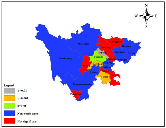
Figure 15.
Reliability of local Moran’s I statistic calculation results in 2010.
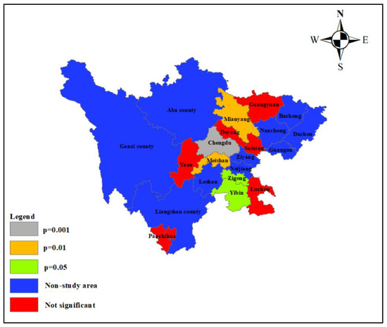
Figure 16.
Reliability of local Moran’s I statistic calculation results in 2015.
Figure 17.
Reliability of local Moran’s I statistic calculation results in 2020.
6. Discussion
The findings in Table 2 suggest that the administrative area, total investment in fixed assets by region, number of employed persons in secondary and tertiary industries, GDP in secondary and tertiary industries, the average wage of staff and workers, basic statistics on per capita park green area, carbon emissions of land, the volume of industrial wastewater discharged, the volume of industrial sulphur dioxide emission, and the volume of industrial soot (dust) emission are critical factors in analysing CGLUE. In contrast to previous studies, this study indicates that the carbon emissions of land should be considered an undesired output [60,61]. With the targets of carbon reduction, economic improvement, and sustainable social development, how much carbon will be generated by each unit of land resource is particularly important [62,63]. The carbon emissions of land can measure land resources’ coal consumption, natural gas emissions, and electricity consumption.
As illustrated by the time-evolution laws shown in Figure 8, Figure 9 and Figure 10, this study has a revolved CGLUE evolution law based on time series. The county’s green land-use efficiency in the 11 counties showed improvement. The main reason for this is that Sichuan Province established the concept of a park city, and the economic development of the city considers the green environment and social sustainability. For example, Figure 10 shows a peak in 2020. There are several reasons for this peak. First, in terms of air-quality improvement, Sichuan Province realised the whole-chain supervision of trucks delivering gas. Second, vehicles transporting concrete can transport no more than 5 tons per trip. Third, Sichuan accelerated the improvement in the urban green travel system and strengthened the integrated development and efficient operation of rail and public transport to reduce carbon emissions and advocate for green travel.
As shown in Table 3 regarding the analysis of spatial evolution law, the Global Moran’s I statistic of CGLUE increased first and then decreased. The reasons for the increased CGLUE include Sichuan Province’s acceleration of the promotion of urbanisation and the integrated development of the whole region. Moreover, Sichuan Province coordinated the construction of the South Sichuan, Northeast Sichuan, Panxi Economic Zone, and Northwest Sichuan Ecological Demonstration Zone. The two measures above mean that the spatial agglomeration of CGLUE continued to increase. However, in 2020, the global Moran’s I statistics of CGLUE decreased to 0.428, which reflected the change in the spatial agglomeration state from strong to weak, indicating that the difference in CGLUE between regions expanded because of COVID-19. However, overall, Sichuan Province CGLUE still maintained a high spatial concentration.
As represented by the spatial evolution law in Figure 12, Figure 13 and Figure 14, the high–low CGLUE agglomeration areas are increasing, and many resources of Sichuan province are gathered in Chengdu. Chengdu, Mianyang, Meishan, and Yibin, which had a high effect from 2010 to 2020, continued to influence Deyang, Yaan, and Zigong, which had a low effect. This result is highly consistent with reality. Sichuan Province highlights the coordinated development of Chengdu, Deyang, Meishan, and Zigong in Sichuan Province’s 14th Five-Year Plan Report. These counties’ resources are flowing and interacting at high speed.
7. Conclusions
China is in the process of high-quality development, and it is increasing its green urbanisation. Sichuan Province’s urbanisation has introduced various significant changes to urban morphology. In exploring the relationship between green urbanisation and land-use efficiency, this study contributes to our understanding of the time and spatial evolution law of 11 CGLUE counties. The following conclusions can be drawn.
The findings show that the CGLUE factors are the administrative area, total investment in fixed assets by region, number of employed persons in secondary and tertiary industries, GDP in secondary and tertiary industries, the average wage of staff and workers, basic statistics on per capita park green area, carbon emissions of land, the volume of industrial wastewater discharged, the volume of industrial sulphur dioxide emission, and the volume of industrial soot (dust) emission. This study gives more attention to the carbon emissions of land compared to previous studies, which measured the carbon emissions of land resources.
Each county’s green land-use efficiency was analysed. For example, the green land-use efficiency in Chengdu continued to rise from 1.273 in 2010 to 2.434 in 2018 and reduced from 1.648 in 2019 to 1.095 in 2020. The values of CGLUE are all greater than 1, and the peak of the kernel density curve is at a relatively high level. The high level of efficiency and the curve value are growing, which shows that the overall level of Chengdu’s land use is efficient.
From the time-evolution perspective, the overall level of the 11 counties’ green land-use efficiency has been explored. The peak value of the kernel density curve is always at a high level, and the interval on the right side of the curve continues to decrease, indicating that the overall level of Sichuan Province in 11 counties’ green land-use efficiency is growing.
From the spatial evolution perspective, the global Moran’s I statistic of the CGLUE is greater than 0, which indicates that CGLUE has a positive influence on the spatial distribution characteristic. The spatial aggregation of CGLUE continued to increase from 2010 to 2019 and decreased in 2020. The spatial agglomeration state went from strong to weak, indicating that the differences in CGLUE expanded but are not obvious. The 11 counties kept a higher spatial aggregation of CGLUE.
From the spatial evolution perspective, the local Moran’s I statistic of the CGLUE represents both the high–low and low–low types. The high–low CGLUE agglomeration areas are mainly distributed in Chengdu, Mianyang, Meishan, and Yibin. The low–low CGLUE agglomeration areas are mainly distributed in Deyang, Yaan, and Zigong. These high and low CGLUE agglomeration areas show the high-speed exchange of resources in recent years and that the CGLUE gap between counties is shrinking and converging.
8. Limitations and Future Directions of Research Work
There are also several limitations to this study and future directions for the CGLUE. First, with the development of urbanisation, resources, expected output, and undesired output will continue to be dynamic. This study has only analysed county green land-use efficiency from 2010 to 2020, which can only provide near-term management advice for county managers. Therefore, the dynamic database should be further discussed. Second, this study has analysed 11 counties located in Sichuan Province, and the study areas could be expanded in the future.
Supplementary Materials
The following supporting information can be downloaded at: https://www.mdpi.com/article/10.3390/buildings12060816/s1, Table S1: CGLUE factors values of 11 counties in 2010. Table S2: CGLUE factors values of 11 counties in 2011. Table S3: CGLUE factors values of 11 counties in 2012. Table S4: CGLUE factors values of 11 counties in 2013. Table S5: CGLUE factors values of 11 counties in 2014. Table S6: CGLUE factors values of 11 counties in 2015. Table S7: CGLUE factors values of 11 counties in 2016. Table S8: CGLUE factors values of 11 counties in 2017. Table S9: CGLUE factors values of 11 counties in 2018. Table S10: CGLUE factors values of 11 counties in 2019. Table S11: CGLUE factors values of 11 counties in 2020. Table S12: 11 Counties CGLUE from 2010 to 2020.
Author Contributions
Conceptualization: T.Y.; methodology: T.Y.; software, J.Z.; validation: T.Y., J.Z. and Y.X.; Formal analysis, T.Y.; investigation, L.L.; resources, J.Z.; data curation, T.Y.; writing—original draft preparation, T.Y.; writing—review and editing, T.Y.; visualization, T.Y.; supervision, J.Z.; project administration, T.Y.; funding acquisition, T.Y. All authors have read and agreed to the published version of the manuscript.
Funding
The work described in this paper was fully supported by a school project (grant no. RZ2100000776).
Institutional Review Board Statement
Not applicable.
Informed Consent Statement
Not applicable.
Data Availability Statement
The data presented in this study are available on request from the corresponding author.
Conflicts of Interest
The authors declare no conflict of interest.
References
- Halleux, J.-M.; Marcinczak, S.; van der Krabben, E. The adaptive efficiency of land use planning measured by the control of urban sprawl. The cases of the Netherlands, Belgium and Poland. Land Use Policy 2012, 29, 887–898. [Google Scholar] [CrossRef]
- Bala, R.; Prasad, R.; Yadav, V.P. Quantification of urban heat intensity with land use/land cover changes using Landsat satellite data over urban landscapes. Theor. Appl. Climatol. 2021, 145, 1–12. [Google Scholar] [CrossRef]
- Abduljabbar, R.L.; Liyanage, S.; Dia, H. The role of micro-mobility in shaping sustainable cities: A systematic literature review. Transp. Res. Part D Transp. Environ. 2021, 92, 102734. [Google Scholar] [CrossRef]
- Chakraborty, S.; Maity, I.; Dadashpoor, H.; Novotny, J.; Banerji, S. Building in or out? Examining urban expansion patterns and land use efficiency across the global sample of 466 cities with million plus inhabitants. Habitat Int. 2022, 120, 102503. [Google Scholar] [CrossRef]
- Steurer, M.; Bayr, C. Measuring urban sprawl using land use data. Land Use Policy 2020, 97, 104799. [Google Scholar] [CrossRef]
- Rozum, R.I.; Liubezna, I.V.; Kalchenko, O. Improving efficiency of using agricultural land. Sci. Bull. Polissia 2017, 1, 193–196. [Google Scholar] [CrossRef][Green Version]
- Herzig, A.; Nguyen, T.T.; Ausseil, A.-G.E.; Maharjan, G.R.; Dymond, J.R.; Arnhold, S.; Koellner, T.; Rutledge, D.; Tenhunen, J. Assessing resource-use efficiency of land use. Environ. Model. Softw. 2018, 107, 34–49. [Google Scholar] [CrossRef]
- Ferreira, M.D.P.; Féres, J.G. Farm size and Land use efficiency in the Brazilian Amazon. Land Use Policy 2020, 99, 104901. [Google Scholar] [CrossRef]
- Jiang, X.; Lu, X.; Liu, Q.; Chang, C.; Qu, L. The effects of land transfer marketization on the urban land use efficiency: An empirical study based on 285 cities in China. Ecol. Indic. 2021, 132, 108296. [Google Scholar] [CrossRef]
- Wang, S.; Cebula, R.J.; Liu, X.; Foley, M. Housing prices and urban land use efficiency. Appl. Econ. Lett. 2021, 28, 1121–1124. [Google Scholar] [CrossRef]
- Dinda, S.; Das Chatterjee, N.; Ghosh, S. An integrated simulation approach to the assessment of urban growth pattern and loss in urban green space in Kolkata, India: A GIS-based analysis. Ecol. Indic. 2020, 121, 107178. [Google Scholar] [CrossRef]
- Liu, S.; Xiao, W.; Li, L.; Ye, Y.; Song, X. Urban land use efficiency and improvement potential in China: A stochastic frontier analysis. Land Use Policy 2020, 99, 105046. [Google Scholar] [CrossRef]
- Bozdag, A.; Inam, S. Collaborative land use planning in urban renewal. J. Urban Reg. Anal. 2021, 13, 323–342. [Google Scholar] [CrossRef]
- Raman, R.; Roy, U.K. Taxonomy of urban mixed land use planning. Land Use Policy 2019, 88, 104102. [Google Scholar] [CrossRef]
- Anugraha, A.S.; Chu, H.-J.; Ali, M.Z. Social sensing for urban land use identification. ISPRS Int. J. Geo-Inf. 2020, 9, 550. [Google Scholar] [CrossRef]
- Den, X.Z.; Gibson, O. Sustainable land use management for improving land eco-efficiency: A case study of Hebei, China. Ann. Oper. Res. 2020, 290, 265–277. [Google Scholar]
- Ghosh, P.A.; Raval, P.M. Modelling urban mixed land-use prediction using influence parameters. GeoScape 2021, 15, 66–78. [Google Scholar] [CrossRef]
- Jalilov, S.-M.; Chen, Y.; Quang, N.; Nguyen, M.; Leighton, B.; Paget, M.; Lazarow, N. Estimation of urban land-use efficiency for sustainable development by integrating over 30-year landsat imagery with population data: A case study of Ha Long, Vietnam. Sustainability 2021, 13, 8848. [Google Scholar] [CrossRef]
- Masini, E.; Tomao, A.; Barbati, A.; Corona, P.; Serra, P.; Salvati, L. Urban growth, land-use efficiency and local socioeconomic context: A comparative analysis of 417 metropolitan regions in Europe. Environ. Manag. 2019, 63, 322–337. [Google Scholar] [CrossRef]
- Adintsova, N.P.; Yelfimova, Y.M.; Zhuravleva, E.P.; Levushkina, S.V.; Chernobay, N.B. Ecological and economic efficiency use of agricultural lands. Res. J. Pharm. Biol. Chem. Sci. 2018, 9, 1316–1330. [Google Scholar]
- Noda, K.; Iida, A.; Watanabe, S.; Osawa, K. Efficiency and sustainability of land-resource use on a small island. Environ. Res. Lett. 2019, 14, 054004. [Google Scholar] [CrossRef]
- Zitti, M.; Ferrara, C.; Perini, L.; Carlucci, M.; Salvati, L. Long-term urban growth and land use efficiency in Southern Europe: Implications for sustainable land management. Sustainability 2015, 7, 3359–3385. [Google Scholar] [CrossRef]
- Saikku, L.; Mattila, T.J. Drivers of land use efficiency and trade embodied biomass use of Finland 2000–2010. Ecol. Indic. 2017, 77, 348–356. [Google Scholar] [CrossRef]
- Shan, L.; Jiang, Y.; Liu, C.; Wang, Y.; Zhang, G.; Cui, X.; Li, F. Exploring the multi-dimensional coordination relationship between population urbanization and land urbanization based on the MDCE model: A case study of the Yangtze River Economic Belt, China. PLoS ONE 2021, 16, e0253898. [Google Scholar] [CrossRef]
- Fetzel, T.; Gradwohl, M.; Erb, K.H. Conversion, intensification, and abandonment: A human appropriation of net primary production approach to analyze historic land-use dynamics in New Zealand 1860–2005. Ecol. Econ. 2014, 97, 201–208. [Google Scholar] [CrossRef]
- Searchinger, T.D.; Wirsenius, S.; Beringer, T.; Dumas, P. Assessing the efficiency of changes in land use for mitigating climate change. Nature 2018, 564, 249–253. [Google Scholar] [CrossRef]
- Tan, S.; Hu, B.; Kuang, B.; Zhou, M. Regional differences and dynamic evolution of urban land green use efficiency within the Yangtze River Delta, China. Land Use Policy 2021, 106, 105449. [Google Scholar] [CrossRef]
- Guastella, G.; Pareglio, S.; Sckokai, P. A spatial econometric analysis of land use efficiency in large and small municipalities. Land Use Policy 2017, 63, 288–297. [Google Scholar] [CrossRef]
- Yang, K.; Zhong, T.; Zhang, Y.; Wen, Q. Total factor productivity of urban land use in China. Growth Chang. 2020, 51, 1784–1803. [Google Scholar] [CrossRef]
- Attardi, R.; Cerreta, M.; Sannicandro, V.; Torre, C.M. Non-compensatory composite indicators for the evaluation of urban planning policy: The land-use policy efficiency index (LUPEI). Eur. J. Oper. Res. 2018, 264, 491–507. [Google Scholar] [CrossRef]
- Zhang, X.P.; Lu, X.H.; Chen, D.L.; Zhang, C.Z.; Ge, K.; Kuang, B.; Liu, S. Is environmental regulation a blessing or a curse for China’s urban land use efficiency? Evidence from a threshold effect model. Growth Chang. 2021, 52, 265–282. [Google Scholar] [CrossRef]
- Tang, Y.; Wang, K.; Ji, X.; Xu, H.; Xiao, Y. Assessment and spatial-temporal evolution analysis of urban land use efficiency under green development orientation: Case of the Yangtze River delta urban agglomerations. Land 2021, 10, 715. [Google Scholar] [CrossRef]
- Zhu, X.; Zhang, P.; Wei, Y.; Li, Y.; Zhao, H. Measuring the efficiency and driving factors of urban land use based on the DEA method and the PLS-SEM model-A case study of 35 large and medium-sized cities in China. Sustain. Cities Soc. 2019, 50, 101646. [Google Scholar] [CrossRef]
- Fetzel, T.; Niedertscheider, M.; Haberl, H.; Krausmann, F.; Erb, K.-H. Patterns and changes of land use and land-use efficiency in Africa 1980–2005: An analysis based on the human appropriation of net primary production framework. Reg. Environ. Chang. 2015, 16, 1507–1520. [Google Scholar] [CrossRef]
- Pang, X.; Wang, D.; Zhang, F.; Wang, M.; Cao, N. The spatial-temporal differentiation of green land use in Beijing-Tianjin-Hebei urban agglomeration. Chin. J. Popul. Resour. Environ. 2018, 16, 343–354. [Google Scholar] [CrossRef]
- Li, C.; Cai, G.; Du, M. Big data supported the identification of urban land efficiency in eurasia by indicator SDG 11.3.1. ISPRS Int. J. Geo-Inf. 2021, 10, 64. [Google Scholar] [CrossRef]
- Liu, Z.; Zhang, L.; Rommel, J.; Feng, S. Do land markets improve land-use efficiency? evidence from Jiangsu, China. Appl. Econ. 2020, 52, 317–330. [Google Scholar] [CrossRef]
- Huang, J.; Xue, D. Study on temporal and spatial variatizon characteristics and influencing factors of land use efficiency in Xi’an, China. Sustainability 2019, 11, 6649. [Google Scholar] [CrossRef]
- Koroso, N.H.; Lengoiboni, M.; Zevenbergen, J.A. Urbanization and urban land use efficiency: Evidence from regional and Addis Ababa satellite cities, Ethiopia. Habitat Int. 2021, 117, 102437. [Google Scholar] [CrossRef]
- Dai, P.; Zhang, S.; Chen, Z.; Gong, Y.; Hou, H. Perceptions of cultural ecosystem services in urban parks based on social network data. Sustainability 2019, 11, 5386. [Google Scholar] [CrossRef]
- Zhao, Y.X.; Cheng, S.X.; Yu, X.Y.; Xu, H.L. Chinese public’s attention to the COVID-19 epidemic on social media: Observational descriptive study. J. Med. Internet Res. 2020, 22, e18825. [Google Scholar] [CrossRef] [PubMed]
- Cook, W.D.; Tone, K.; Zhu, J. Data envelopment analysis: Prior to choosing a model. Omega 2014, 44, 1–4. [Google Scholar] [CrossRef]
- Sueyoshi, T.; Yuan, Y.; Goto, M. A literature study for DEA applied to energy and environment. Energy Econ. 2016, 62, 104–124. [Google Scholar] [CrossRef]
- Hatami-Marbini, A.; Emrouznejad, A.; Tavana, M. A taxonomy and review of the fuzzy data envelopment analysis literature: Two decades in the making. Eur. J. Oper. Res. 2011, 214, 457–472. [Google Scholar] [CrossRef]
- Emrouznejad, A.; Yang, G.-L. A survey and analysis of the first 40 years of scholarly literature in DEA: 1978–2016. Socio-Econ. Plan. Sci. 2018, 61, 4–8. [Google Scholar] [CrossRef]
- Tone, K.; Tsutsui, M. Dynamic DEA with network structure: A slacks-based measure approach. Omega 2014, 42, 124–131. [Google Scholar] [CrossRef]
- Mahmoudi, R.; Emrouznejad, A.; Shetab-Boushehri, S.-N.; Hejazi, S.R. The origins, development and future directions of data envelopment analysis approach in transportation systems. Socio-Econ. Plan. Sci. 2020, 69, 100672. [Google Scholar] [CrossRef]
- Choi, Y.; Zhang, N.; Zhou, P. Efficiency and abatement costs of energy-related CO2 emissions in China: A slacks-based efficiency measure. Appl. Energy 2012, 98, 198–208. [Google Scholar] [CrossRef]
- O’Brien, T.A.; Kashinath, K.; Cavanaugh, N.R.; Collins, W.; O’Brien, J.P. A fast and objective multidimensional kernel density estimation method: FastKDE. Comput. Stat. Data Anal. 2016, 101, 148–160. [Google Scholar] [CrossRef]
- Helu, A.; Samawi, H.; Rochani, H.; Yin, J.; Vogel, R. Kernel density estimation based on progressive type-II censoring. J. Korean Stat. Soc. 2020, 49, 475–498. [Google Scholar] [CrossRef]
- Goldenshluger, A.; Lepski, O. Bandwidth selection in kernel density estimation: Oracle inequalities and ADAPTIVE MINIMAX optimality. Ann. Stat. 2011, 39, 1608–1632. [Google Scholar] [CrossRef]
- Jeon, J.; Taylor, J.W. Using conditional kernel density estimation for wind power density forecasting. J. Am. Stat. Assoc. 2012, 107, 66–79. [Google Scholar] [CrossRef]
- Calonico, S.; Cattaneo, M.D.; Farrell, M.H. On the effect of bias estimation on coverage accuracy in nonparametric inference. J. Am. Stat. Assoc. 2018, 113, 767–779. [Google Scholar] [CrossRef]
- Baddeley, A.; Nair, G.; Rakshit, S.; McSwiggan, G.; Davies, T.M. Analysing point patterns on networks—A review. Spat. Stat. 2021, 42, 100435. [Google Scholar] [CrossRef]
- Bilal, U.; Tabb, L.P.; Barber, S.; Roux, A.V.D. Spatial inequities in COVID-19 testing, positivity, confirmed cases, and mortality in 3 US cities an ecological study. Ann. Intern. Med. 2021, 174, 936–944. [Google Scholar] [CrossRef]
- Islam, A.; Abu Sayeed, M.; Rahman, M.K.; Ferdous, J.; Islam, S.; Hassan, M.M. Geospatial dynamics of COVID-19 clusters and hotspots in Bangladesh. Transbound. Emerg. Dis. 2021, 68, 3643–3657. [Google Scholar] [CrossRef]
- Lima, R.C.D.A.; Resende, G.M. Using the Moran’s I to detect bid rigging in Brazilian procurement auctions. Ann. Reg. Sci. 2020, 66, 237–254. [Google Scholar] [CrossRef]
- Bivand, R.S.; Wong, D.W.S. Comparing implementations of global and local indicators of spatial association. Test 2018, 27, 716–748. [Google Scholar] [CrossRef]
- Aghadadashi, V.; Molaei, S.; Mehdinia, A.; Mohammadi, J.; Moeinaddini, M.; Bakhtiari, A.R. Using GIS, geostatistics and Fuzzy logic to study spatial structure of sedimentary total PAHs and potential eco-risks; An eastern persian gulf case study. Mar. Pollut. Bull. 2019, 149, 110489. [Google Scholar] [CrossRef]
- Scharlemann, J.; Tanner, E.V.; Hiederer, R.; Kapos, V. Global soil carbon: Understanding and managing the largest terrestrial carbon pool. Carbon Manag. 2014, 5, 81–91. [Google Scholar] [CrossRef]
- Ciais, P.; Tan, J.; Wang, X.; Roedenbeck, C.; Chevallier, F.; Piao, S.-L.; Moriarty, R.; Broquet, G.; Le Quéré, C.; Canadell, J.G.; et al. Five decades of northern land carbon uptake revealed by the interhemispheric CO2 gradient. Nature 2019, 568, 221–225. [Google Scholar] [CrossRef] [PubMed]
- Houghton, R.A.; House, J.I.; Pongratz, J.; Van Der Werf, G.R.; DeFries, R.S.; Hansen, M.C.; Le Quéré, C.; Ramankutty, N. Carbon emissions from land use and land-cover change. Biogeosciences 2012, 9, 5125–5142. [Google Scholar] [CrossRef]
- Ahmad, M.; Rehman, A.; Shah, S.A.A.; Solangi, Y.A.; Chandio, A.A.; Jabeen, G. Stylized heterogeneous dynamic links among healthcare expenditures, land urbanization, and CO2 emissions across economic development levels. Sci. Total Environ. 2021, 753, 142228. [Google Scholar] [CrossRef] [PubMed]
Publisher’s Note: MDPI stays neutral with regard to jurisdictional claims in published maps and institutional affiliations. |
© 2022 by the authors. Licensee MDPI, Basel, Switzerland. This article is an open access article distributed under the terms and conditions of the Creative Commons Attribution (CC BY) license (https://creativecommons.org/licenses/by/4.0/).