Abstract
The noise effects in the room impulse response (RIR) make the decay range of the integrated impulse response insufficient for reliable determination of reverberation time (RT). One of the preferred techniques to minimize noise effects is based on noise subtraction, RIR truncation, and correction for the truncation. The success of RT estimation through the method depends critically on the accurate estimation of the truncation time (TT). However, noise fluctuation and RIR irregularities can lead to discrepancies in the determined TT from the optimal value. The general goal of this paper is to improve RT estimates. An iterative procedure based on a non-exponential decay model consisting of a double-slope decay term and a noise term is presented to estimate the TT accurately. The model parameters are generated until the iterative procedure converges to a minimum difference between the energy decay curve (EDC) generated by the model and the Schroeder decay function. The decay rates of the EDCs with added pink noise levels are compared to those of the EDCs with low background noise. In addition, the detected TTs and the corresponding RTs are compared with the existing method and the noise compensation method (subtraction–truncation–correction method).
1. Introduction
The reverberation time (RT) is the most representative and physically important parameter related to the average properties of a room [1,2,3]. Hence, it is essential for predicting speech intelligibility [4,5]. The well-known and widely used method to calculate RT is determined by the energy decay curve (EDC) generated by Schroeder’s method [6]. However, the ambient and equipment noise is always present in environments, occurring in the room impulse response (RIR) during measurements [7]. The noise may lead to a characteristic curvature in the EDC [8,9]. Therefore, the dynamic range of the EDC is insufficient for the reliable determination of RT. To overcome the problem, studies and achievements were proposed to mitigate insufficient dynamic ranges in the Schroeder decay functions [10,11,12,13,14,15]. The typical research emphasized truncating the RIR at a time point to generate noise-free decay curves [12,13]. Although various times can be used for RIR truncation, only the time where the main decay slope intersects with the noise floor level representing the optimal truncation time (TT) gives the correct decay slope and RT [14,15]. The relative error of the RT of the measured RIR will be greater than 5% when the deviation of the TT from the optimal TT is larger than 10% [16].
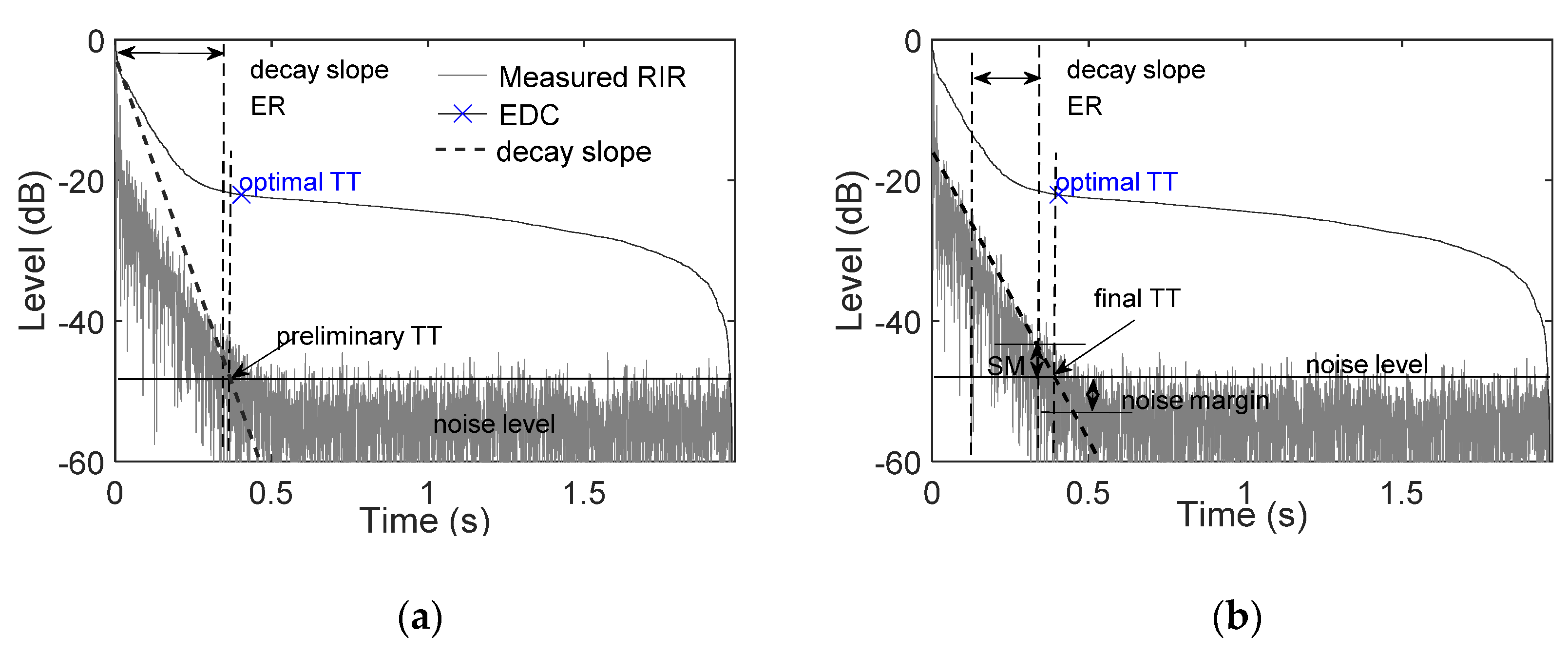
Precise determination of TT is difficult in practice. According to the research [16], the TT can be manually determined by a simple method of an intersection of the main decay slope and the noise floor level. However, the non-exponential decay and the characteristic curvature in the EDC make the decay slope dependent on the ER [8,15], as seen in the decay slope (black dotted curve) in Figure 1. Observing Figure 1a, when the measured RIR has high initial peaks, the corresponding EDC presents a non-exponential decay behavior. The decay slope estimated in the ER, ranging from the beginning of the RIR to a certain point some dBs above the assumed noise level, is decreased, resulting in a smaller value of the preliminary TT than the optimal TT. In order to reduce the influence of the non-exponential decay of the EDC on the decay slope estimation, the ER can be manually adjusted using an additional slope margin (SM) and a noise margin [15]. In the case presented in Figure 1b, the influence of the initial peak of the RIR on the decay slope is decreased, causing the generated final TT close to the optimal TT.
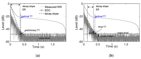
Figure 1.
Detection of TT dependent on the ER: (a) the preliminary TT generated from the estimated ER; (b) the final TT generates from the ER with a selection slope margin and noise margin.
Despite the optimal TT detected, the characteristic curvature in the EDC results in an error in the RT determination. In this case, the PNR, depending on the final TT, prescribes a maximum decay range for the measurement of T30. However, the relative error of the T30 estimated in the decay range of the EDC is over 20%. It has been illustrated that without noise compensation, the relative error of the RT is approximately 16% or even larger [14,17]. That is why one must pay special attention to the noise compensation since the decay curve can be automatically limited to its reliable dynamic range according to the actual SNR [14]. However, the truncation effects in the EDC are approaching minus infinity at the TT, causing a severe underestimation of the RT for low SNR. The error of RT determination caused by improper truncation depends on the TT displacement. Thus, Lundeby et al. [10] proposed a correction term to prevent the effects. The correction part assumes an exponential decay, which should be the same as the decay slope of the estimation range (ER) ranging from the TT to a certain point [9,10]. However, this range has been influenced by noise since the signal and noise energy are equal at the TT. Furthermore, the fluctuation in the noise tail of the RIR or different segment size may cause different estimations of the mean-square values of the noise levels, complicating the ERs determination. Considering the decay slope depends on the ER, the error will cause the TT to deviate from the optimal value.
In order to counteract the noise estimation influence in TT detection, techniques based on the energy–time curve analysis of the signal envelope are proposed since the noise level can be found and explicitly estimated [17,18]. A nonlinear decay model that consists of an exponential decay plus noise is fitted to energy–time functions of the measured RIR by applying the least-squares (LS) optimization to automatedly determine the TT [8,19]. Nevertheless, the model still leaves some uncertainty in the measured RIR with non-exponential decay. The deviation of the detected TT from the optimal value can also be large when the measured RIR has double-slope decay behavior [8,18]. In order to improve the ability of TT detection in more complex cases, the nonlinear decay model expressed in multiple-slope decay terms in terms of the Bayesian analysis may be more suited to describe the Schroeder decay functions in practicality [20,21]. Besides these mathematical methods, studies based on signal techniques have been developed to de-noising the RIRs to improve the dynamic range of the EDC [16,22]. These de-noising procedures rely on the accurate estimation of the TT.
Considering the high initial peaks and early reflections of measured RIRs, a noise compensation procedure is combined with a nonlinear regression model with multiple-slope decay terms and a noise term to decrease the RIR irregularities and noise uncertainty in the TT determination. The model parameters, including the noise level LN and start level , automatically define the ER related to the TT. The procedure automatically estimates the model parameters by iteratively minimizing the difference between the EDC of the model and the EDC generated from the RIR given in Section 4. The iterative process leads to convergence to the minimum value by LS optimization estimation of initial parameters after only a few iterations. The investigation is carried out on the measured RIRs with artificial and natural ambient noise. In addition, the proposed procedure for determining the TT and the corresponding RT of measured RIRs is compared with the compensation method.
2. Procedure for Detection of TT
2.1. Nonlienar Regression Model
According to the studies [17,23], the mean-square value of the background noise can be explicitly found and estimated by using a nonlinear regression model. The parameters in the model, including the initial level, noise level, and decay slope can be calculated through LS optimization by fitting the nonlinear decay model to the logarithmic decays of the measured RIRs. The nonlinear decay model consisting of a single exponential decay and stationary noise is proposed to produce a smooth decay envelope to decrease the RIR fluctuation as [8]:
The parameters , , and represent the initial level, the average noise level, and the exponential decay slope, respectively. The envelopes consist of exponential decay and noise, denoted by and . The is constant since the model is related to the stationary background noise in the RIR. The time limits, and , are the lower and the upper limits of the backward integration, respectively. The TT (denoted by ) derives from the model, which can be estimated from the parameters,
The procedure shows that the influence of the fluctuations on the TT determination is almost eliminated. The errors of the model parameters in Equation (1) are minimized by using the LS difference fitting to the integrated model and the EDC of the RIR. However, this model failed to describe the RIR with a non-exponential decay slope, and it led to an estimation error on parameter , causing a significant deviation of the detected TT [19,24].
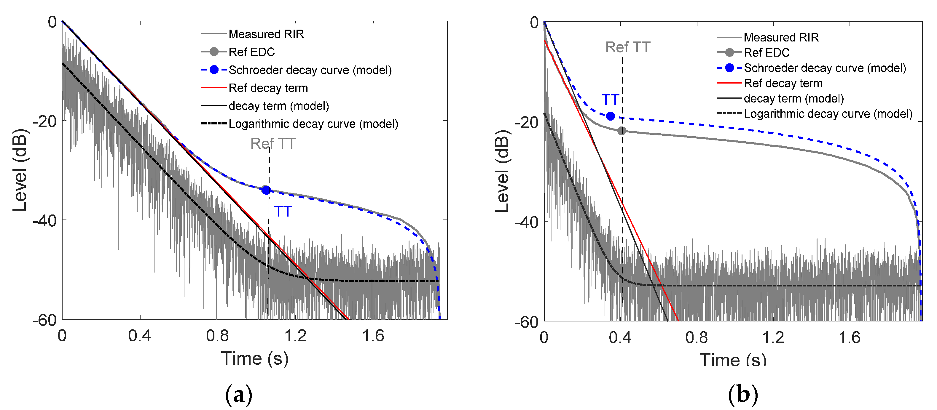
Figure 2 presents the comparison results of the TT detected from the two measured RIR with exponential decay and non-exponential decay between the reference TT. The RIRs measured from rooms B and C (as described in Section 3) are used as inputs in the LS optimization, yielding the model parameters to form the logarithmic decay curves and the corresponding normalized EDCs in terms of the Schroeder decay function. As shown in Figure 2a, the model generates a smooth and a monotone-decreasing decay curve that is well-suited to describe the reference EDC of the measured RIR with truly exponential decay. The decay slope and the noise level are detected more accurately, resulting in a slight deviation between the TT and the reference TT. The relative error of the RTs is approximately 1.6%. However, the EDC resulting from this model fails to describe the reference EDC of the measured RIR with a high initial peak, as shown in Figure 2b. The model causes a shift of the decay curve, leading to a relatively large deviation of the TT. In this case, the relative error of the RTs is up to 8.7%.
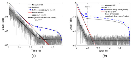
Figure 2.
Logarithmic decay curves (black dotted line) and Schroeder decay curve (blue dotted line) generated from the model (Equation (1)) after applying LS optimization together with the comparison between the reference TT and TT of the model and decay term: (a) Decay curves of the measured RIR (room C) with exponential decay; (b) Decay curves of the measured RIR (room B) with non-exponential decay.
2.2. Non-Exponential Decay Model on TT Detection
The nonlinear decay model of Equation (1), consisting of a single exponential decay and stationary noise in detecting TT, was briefly described. Considering the non-exponential decay behavior of measured RIRs, a solution using non-single-exponential decay model could enable a specific envelope closer to the real one. The single decay term in Equation (1) is considered to extend it to multiple-slope decays to generate a logarithmic envelope of the energy–time functions (RIR expressed in dB), with a non-exponential decay in terms of [17] is expressed as,
The subscript s in the model in Equation (3) is the decay order, denoting the decay model contains s different exponential decay terms with s different decay times. Where is the background noise in dB-scale, is the maximum RMS level in dB-scale.
According to reference [25,26], to define , the backward integration method is as beneficial as it has already proven to be for the accurate determination of the decay slope. The , determining the initial level of the , is defined as the level of the total impulse response energy normalized to the RT expressed as
and
Here, is the maximum impulse response value, and corresponds to each decay term of the . Based on the TT detection function of Equation (2), replacing the and by the (Equation (4)) and , the for j-th decay terms can be expressed as
Even though this procedure can be applied to a virtually unlimited number of slopes, this paper only analyzes the measured RIRs with double-slope decays. The symbol is the TT corresponding to the main decay slope and represents the bending point of the two decay terms [19]. The amplitude parameters , and decay slopes ( are mutually dependent. The displacement of TT from the optimum is demonstrated through the determination of RT, using the noise compensation mentioned in Figure 1. Considering the difficulties of manual adjustment operation in TT, the model Equation (3) incorporated in the noise compensation method [10] is conducted to automated determine the ER by the model parameters and The parameters are iteratively achieved by minimizing the deviation between the decay levels of the EDC at the TT of the measured RIRs and the backward integrated non-exponential decay model Equation (3) in terms of the Schroeder decay model [18,27],
Because the parameters in the model are unknown at the beginning of the iteration, the model parameters in Equation (7) are initially calculated using the LS optimization to fit the model to the Schroeder-integrated energy-time curve, given by [8,23]:
The LS optimization is realized using the MATLAB function (fminsearch) [24]. The LS optimization can also be realized using the MATLAB function (lscurvefit) [8]. The results of the parameters are applied in Equation (6) to form an EDC and to estimate the . The absolute value between the decay level of the logarithmic backward integrated model and the logarithmic backward integrated measured RIR is calculated. The iterative procedures will lead to convergence to the local minimum after only a few iterations [10]. When the absolute value exceeds approximately 0.5 dB [19], the iteration stops. The decay level difference between the decay level of the TT of the model and the measured RIR is applied to redefine the end level of the ER. The optimal TT is detected when the difference approaches zero or meets an acceptable threshold. The procedures are analyzed in detail in Section 4.2.
3. Implementation and Experimentation
The investigation in this paper was carried out using real measured RIRs to analyze and to confirm the performance and the feasibility of the proposed procedure for TT detection and RT estimation. The premise is that the parameters in the model can fully describe the backward integrated decay curve of a measured RIR. The measured RIRs are achieved from rooms with three different structures, which shows that the approach can work in rooms with various acoustic features. The proposed procedure fits the model to the EDC of the noisy RIRs, and it verifies the accuracy of the obtained TTs and RTs. The results are compared with the noise compensation method with noise subtraction, RIR truncation, and correction for the truncation [14,17]. The RT is calculated from the decay slope of the regression line over the decay range of the generated EDCs. The decay range starts at −5 dB to the decay level of the optimal , which is the case throughout the paper [9]. The process was developed in MATLAB for the calculation and optimal TT determination of the model parameters.
Artificial pink noise at different levels (from −60 dB to −40 dB in −5 dB steps) was added to the RIRs to produce various dynamic ranges and SNRs. The reason for using these RIRs is that the structures of the three rooms are different, and the background noise is low enough to add artificial noise. In addition, the acoustic parameters obtained from low background noise are more accurate than those with high background noise, enabling reliable evaluation. The meeting room (Room A) is a lecture theatre with approximate dimensions of 16.5 × 4.35 × 9.95 and 130 seats. The room is equipped with perforated plates, mineral–wool sound-absorbing board, and a marble floor. Although it is a single large room, the various absorption materials and specific structures produce a measured RIR with a strong direct sound. The generated decay curve is a non-exponential decay with double decay terms. The laboratory (Room B) is a simple room with a main rectangular volume with dimensions of 12 × 10 × 3.8 . The measured RIRs have double decay terms. The third room (Room C) is a common single classroom of approximately 12 × 9 × 3.2 . The measured RIR has a single-slope decay term. The design of the experiments follows the ISO 3382-1:2009 [9] to evaluate the reference RTs for three rooms. Four positions were used to measure the RIRs in the meeting room and laboratory, and three positions were used in the classroom, yielding fifty-one conditions to verify the model.
4. Analysis of the Proposed Procedure
Important factors in determination of the iterative procedure include the characteristics of RIR and the parameters that define the ER. In order to mitigate the effects of changing time iterative on the ER, the iterative procedure based on the model in Equation (7) is applied in an automated way that can fully estimate the ER related to the optimal TT. The model parameter of LN and respectively define the end and the start level of ER. Since the optimal TT gives a small fitting error between the decay levels of the EDCs of the measured RIRs and Equation (7), the model parameters are expected to well-describes the reference EDC of measured RIR. That is, the smaller the shift of the EDC, the more accurate the estimated model parameters, leading to the TT calculated by Equation (6) being close to the optimum. The RIRs measured in the meeting room with the added pink noise level at −50 dB, filtered in the octave band at 1 kHz, are used to present the proposed procedure. Since the actual is unknown in the measured RIR, the TT corresponding to the minimum deviation of the resulting truncated EDC with the reference decay curve is taken as the reference value. In addition, the analysis is based on generating the EDC of the model and the truncated EDCs of the noise compensation method, observing the deviations of these curves from the references.
4.1. Effects of Iterative Procedure on ER Defining
A number of studies focus on the implication of the noise compensation method in detecting TT since the ER of the decay slope can be automatically estimated in every step of the iteration [10,11]. The decay slope is initially estimated in the ER using linear regression between the time interval containing the response of 0-dB peak and the first interval 5–10 dB above the background noise level. A preliminary TT is determined at the intersection of the decay slope and the background noise level. A new time interval length is calculated based on the decay slope in the previous step, and it defines a new ER for decay slope estimation. The TT is generated until the iterative procedure is found to converge (maximum five iterations) [10].
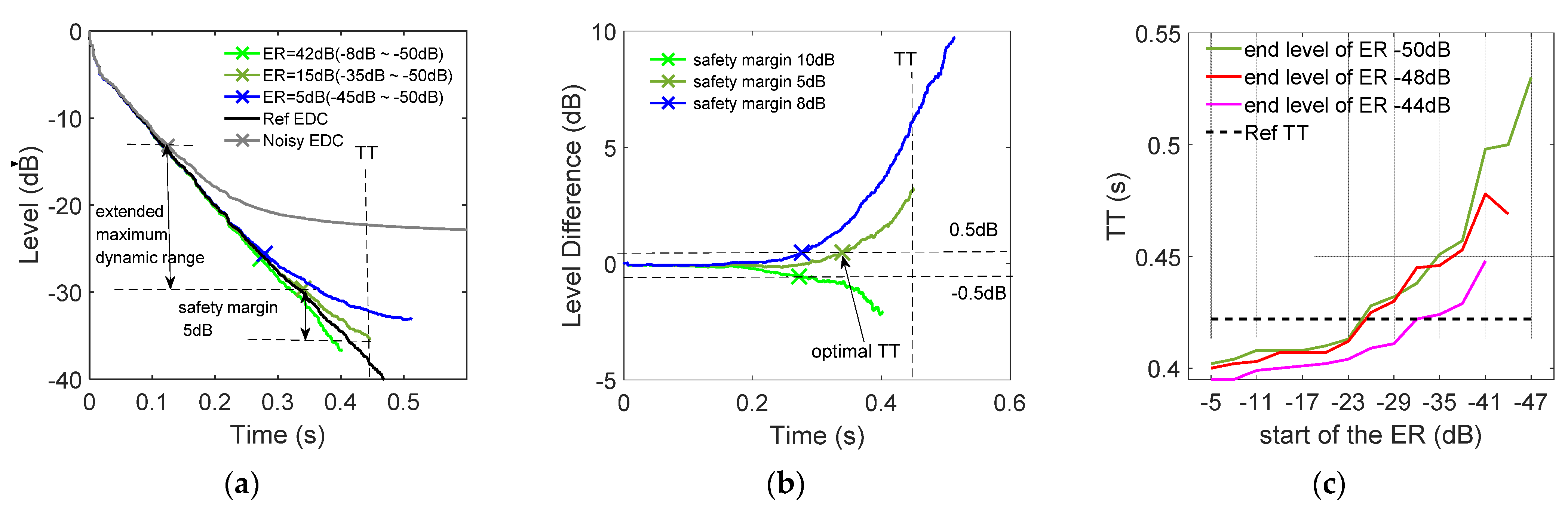
Regarding the truncation process, the optimal TT represents the minimum deviation of the resulting truncated EDC with the reference decay curve, which gives the correct decay slope and RT. Figure 3 presents the truncated EDCs resulting from noise subtraction, RIR truncation at the detected TT, correction term calculated by the TT, and decay slopes of different ER. In the case of an end level of −50 dB given in Figure 3a, the change of the start level of the ER affects the decay slope of the decay curves, causing them to deviate from the reference EDC, thus leading to different TT values. Observing Figure 3c, the closer the start of the ER to the beginning of the RIR, the smaller the detected TT value, leading to a characteristic drop of the EDC tail (green curve). On the other hand, the different pre-setting interval lengths lead to the variable end levels of the ER values (see the green decay curve in Figure 3c). With a fixed start level of the ER, the deviation between the TT and the reference TT increases, with the end level of the ER increasing. In this case, the maximum deviation of the TT is detected when the end of the ER approaches to the estimated mean noise level of −52 dB. The deviation is up to about 10 dB when the last 7 dB is used, as seen in the blue decay curve given in Figure 3b, which is the reason for leaving a safety margin of 5–10 dB above the level corresponding to the TT [9,10].
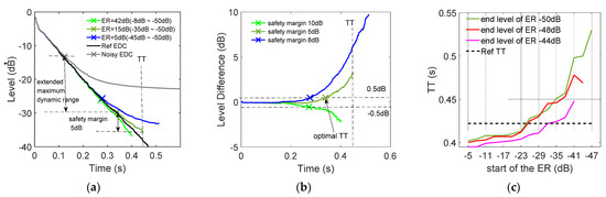
Figure 3.
Truncated EDCs and corresponding TT generated from the noise compensation method: (a) Reference EDC and the truncated EDCs result from the noise compensation method using different RIR ERs. (b) Deviation of the truncated EDC with different ERs given in (a) from the reference EDC. (c) TT was detected from the noise compensation method by using various RIR ERs.
Nevertheless, because the signal and the noise energy are equal at the TT, a deviation of the decay curve also appears even if the RIR is truncated at the actual TT. Figure 3a shows the minimum deviation of the decay curve detected by setting the ER of approximately 15 dB in the case of the end level is −50 dB. To obtain the correct value of RT, it may be possible to exclude the last changed part of the truncated EDC. In most cases, an optimal TT is where the deviation is within 0.5 dB by shifting the TT toward the beginning RIR [16]. This is an expected value, because the contributions of the decay and noise are approximately the same at this time point. The optimal TT resulting in a maximum dynamic range is obtained by using a safety margin of 5 dB [8]. The relative error of the T30 estimated in the truncated EDC above the optimal TT is reduced to 2.1%. Unfortunately, the deviations for the EDCs resulting from the ER of 42 dB and 5 dB are still large, approximately 1.7 dB and 0.9 dB, when using a safety margin of 5 dB. The optimal values of the safety margin for the two cases are about 8 dB and 10 dB. In real measured noisy RIR, it is difficult to determine the safety margin because there is no reference EDC for comparison. The applied safety margin is crucial for the TT determination and the corresponding decay slope estimation.
The pre-setting time interval may lead to variable start and end levels of ER values, especially when the RIR has non-exponential decays. The values will complicate the procedures of TT determination and decay slope estimation. Hence, an automatic algorithm defining the ER for the iterative procedure insensitive to noise level and the irregularities of the RIR is preferable. Furthermore, a strategy to make the truncated EDC above the TT close to the noise-free decay curves is expected.
4.2. Proposed Procedure on TT Detetecting
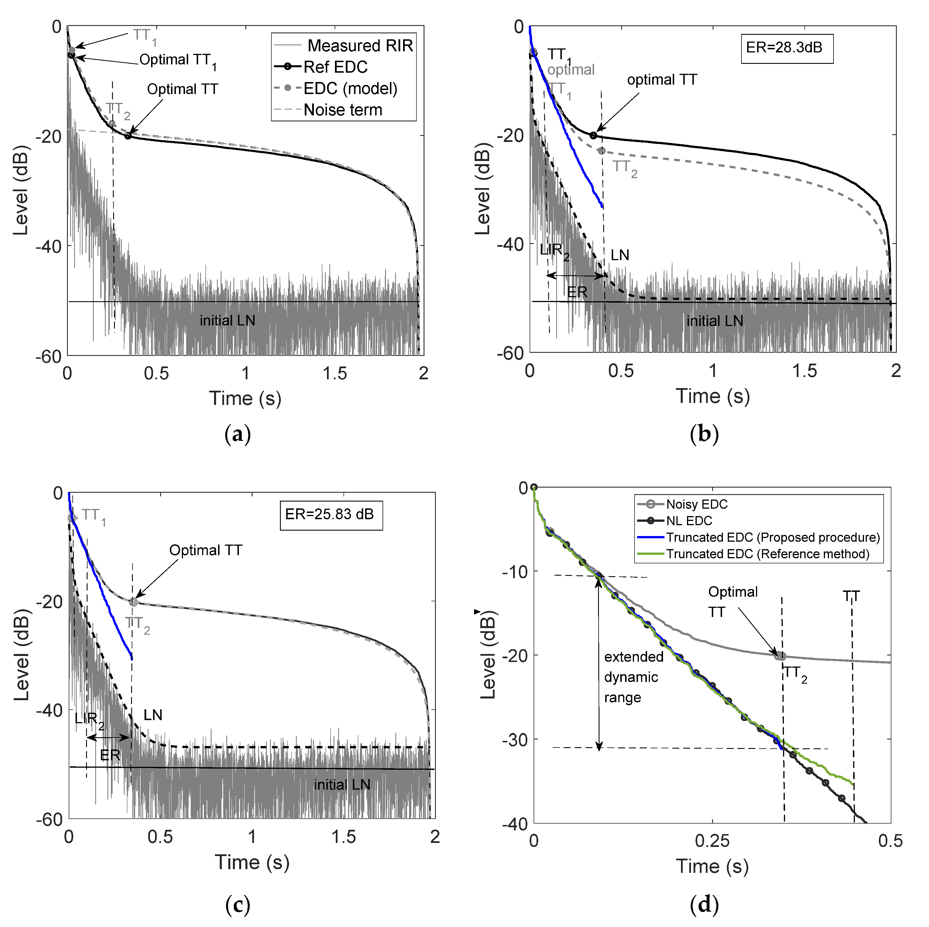
Unlike the first step of the method presented in Section 4.1, the ER of the decay slope and the noise level is unknown at the beginning of the iterative procedure. In the first step of the proposed procedure, the LS optimization fitting the logarithmic backward-integrated model (Equation (3)) to the logarithmic backward-integrated measured RIR provides the initial model parameters. The parameters are applied in Equation (7) and Equation (6) to form an EDC (gray dotted line) and to calculate the initial and , of approximately 0.026 s and 0.253 s, as shown in Figure 4a. It can be noted that the fluctuation of the RIR causes the decay curve to deviate from the reference EDC. Moreover, the fluctuation leads the and the to shift from the optimal value of the and the . In this case, the decay level difference at between the EDC of the model and the reference EDC is 1.1 dB. The estimated error of the is approximately 1.43%. The at the moves down with the level difference to obtain a new one. A new ER from the start RIR to the is obtained to calculate the . The decay level difference at the is up to 2.3 dB. In this case, the decay level difference is implemented to shift the initial LN upward to re-define the end level of the ER. The at the initial is calculated from the initial using Equation (4). Thus, the new ER is approximately 28.3 dB as calculated by the LIR2 and the new LN.
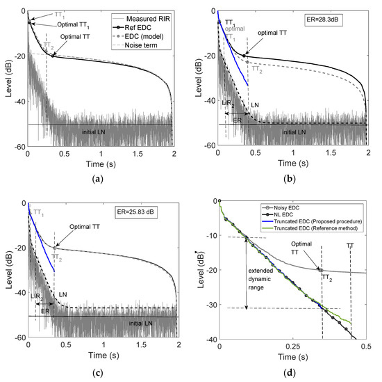
Figure 4.
Comparison of the reference EDC and the EDC obtained from the model given in Equation (7) and corresponding and estimated in Equation (6) by implementing the proposed procedure in each step: (a) The EDC (gray dotted line) generated from the model by using the LS optimization together with the and (b,c) The EDC (gray dotted line) generated from the model by using the parameters from the previous step of the iterative procedure together with the and . (d) comparison of the EDC truncated at the obtained from (c) and the EDC truncated at the given in Section 4.1.
The ER is applied to the iterative procedure to generate a new and a new , and the truncated EDC (blue curve) presented in Figure 4b. The deviation between the detected values and the optimal is decreased. A new is estimated by performing a linear regression of the generated truncated EDC in the range from to , yielding a new LIR2. Implementing those parameters to the model, the newly generated EDC (gray dotted curves) concurs well with the reference EDCs at , but it shifts from the noisy EDC at the , as presented in Figure 4b. The decay level difference at is reduced to approximately 0.09 dB, but the difference at is increased to 4 dB. Observing the LN at the logarithmic energy–time curve (black dotted curve) formed from Equation (3), the value has been influenced by the noise, resulting in a large value of . Because the difference at the is larger than the set absolute value of convergence, approximately 0.5 dB [8,16], the iterative procedure continues as in the previous step.
Finally, the optimal result of the is obtained from the ER of 25.2 dB after four step iterations. The decay curve formed from the model parameters concurs well with the reference EDC presented in Figure 4c. The EDC of the model shows a slight deviation from the reference EDC after 1.4 s. It can be noticed from the ER of the logarithmic energy–time curve that the noise level and the high initial peaks of the RIR have been excluded from the range. Hence, the resulting from the ER and the decay slope is close to the optimal TT generated by the method in Section 4.1. The deviation of the decay curve at the is approximately 0.08 dB, making the relative error of the estimated 0.3%.
The comparison of the truncated EDCs of the reference method and the proposed procedure is presented in Figure 4d. The truncated EDC generated from the ER shown in Figure 4c,d is identical to the NL EDC above the optimal . Section 4.1 has illustrated the complexity of detecting the optimal TT of the reference method. The decay level at the TT is shifted upward to obtain the optimal TT using the safety margin of approximately 5 dB. Nevertheless, the deviation in TT can be automatically excluded from the proposed procedure without applying the safety margin. The deviation at the between the truncated EDC and the NL EDC is only 0.22 dB, leading to a slight increase in the dynamic range. The decay level of the extended to −31 dB. In all the observed cases, the proposed procedure provides a fully automated way to filter out the influence of the random fluctuations and high initial peaks of the RIR on the TT determination.
5. Comparison with Proposed Procedure from Literature
5.1. TT Detection for RIRs with Added Noise
Section 4 presented that the proposed procedure iteratively determines an optimal TT with the model parameters when the non-exponential decay model (Equation (7)) well-describes the Schroeder decay function. Hence, the EDCs formed by the model are considered as a visual inspection to verify the efficiency of the iterative procedure in estimating the parameters in the model (Equation (7)) and TT function (Equation (3)). The measured RIRs are filtered in octave bands with pink noise ranging from −60 dB to −40 dB, which was used to verify the proposed procedure with the non-exponential decay model. The measured EDCs were generated from the RIRs measured at midnight with a low ambient noise level of approximately −66.5 dB. Table 1 presents the model parameters for modeling the EDCs. The decay times (DT) are the decay slope (−13.8/ in the mode [27,28]. The E1 is the decay level of the EDC at the . The parameters ∆E1 and ∆E2 are the decay level differences between the EDC of the model and the reference EDC at the and , respectively. The corresponding NL EDC was produced using the reference noise compensation method, which is taken as a standard to verify the proposed procedure’s effectiveness. In the case of the reference method, the optimal TT values are obtained using safety margins 0–5 dB above the estimated LN. The safety margins are calculated at the time point when the decay level difference between the truncated EDC and the NL EDC is approximately 0.5 dB.

Table 1.
Comparison of DT and TTs between the measured RIRs with added pink noise.
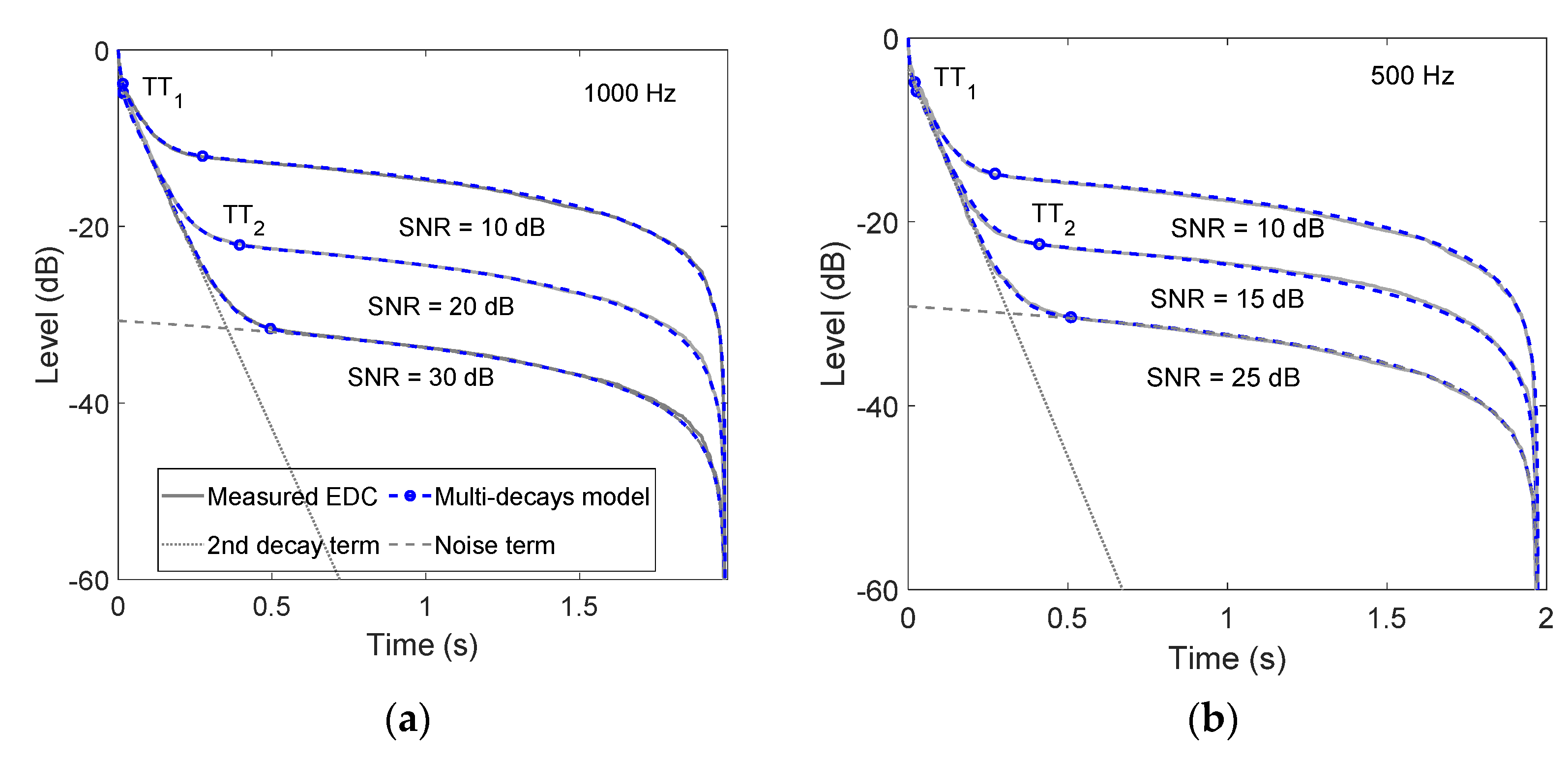
Figure 5 presents the EDCs resulting from the double-slopes decays model with the parameters generated after the proposed procedure, which agree well with the reference EDCs of the measured RIRs at 1000 Hz and 500 Hz with three different resulting SNRs. The decay characteristics represented by these three curves are the same. The decay model curves consist of two exponential decay terms and one noise term. In those EDCs, a rapid decline occurs on the decay curve above . The model describes that part reasonably well, leading to minor shifts at . The ∆E1 presented in Table 1 is below 0.1 dB representing that the is essential for defining the start point of the decay rate . On the other hand, the ∆E2 is below 0.1 dB at , causing the relative error of the estimated DT is less than 0.6% at the 1000 Hz octave band and less than 1.1% at the 500 Hz octave band. The noise term 10log10(shows a tiny shift from the measured EDC near the end of the time, which has less influence on the .
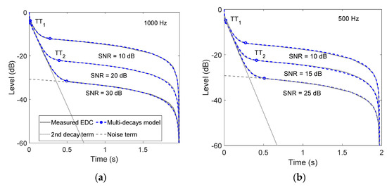
Figure 5.
Comparison of the normalized EDCs generated from the proposed procedure with the non-exponential decay model (Equation (7)) and the measured RIR with added pink noise (−60 dB to −40 dB) and filtered in the octave band at the 1 kHz (a) and 500 Hz (b) octave bands.
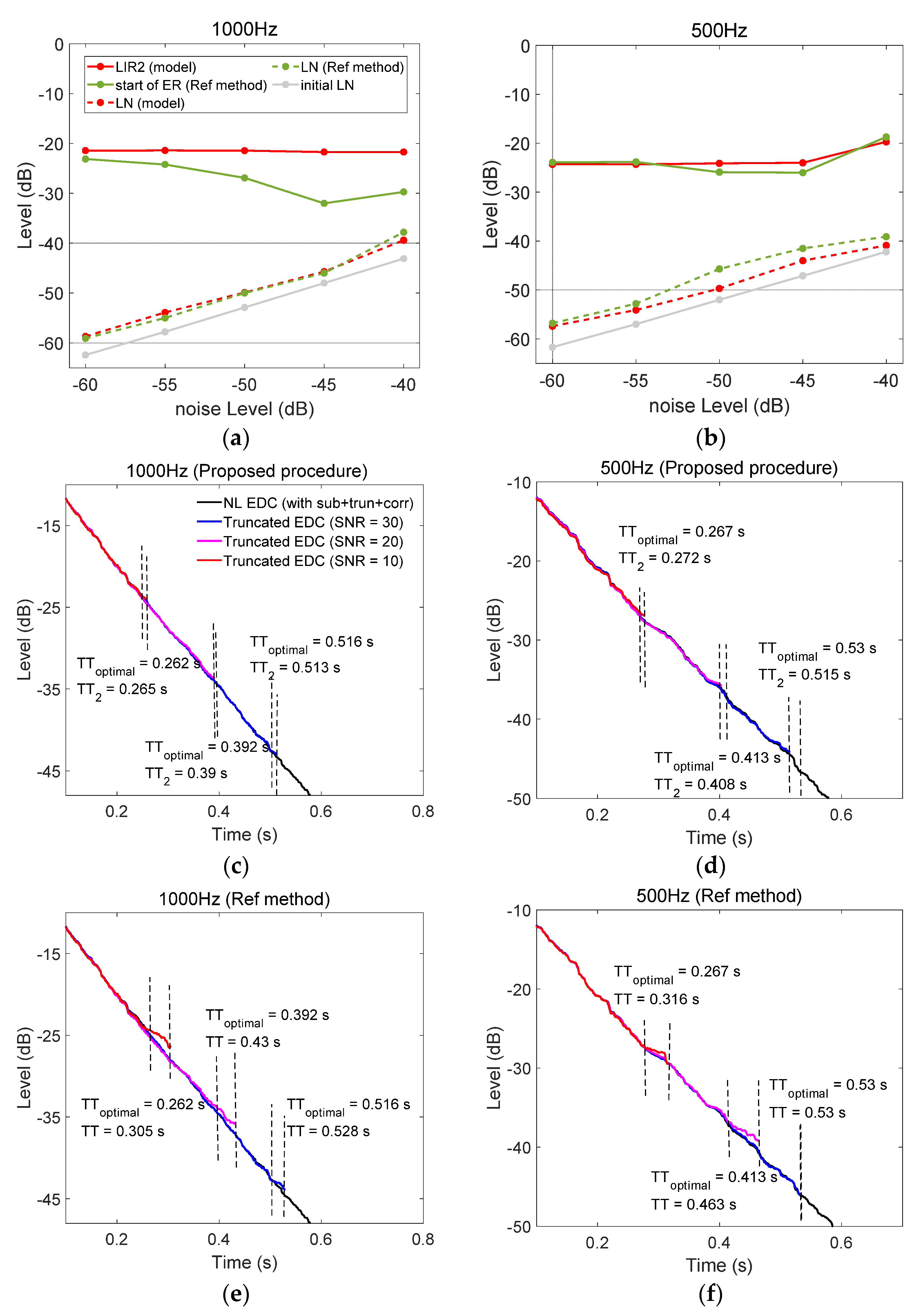
Because the DT estimated from the ER depends on the and the , the correct DTs and the small values of the ∆E1 and the ∆E2 proved that the proposed procedure yields accurate model parameters. Compared to the results presented in Figure 6a,b, the proposed procedure gives somehow stable values of the than those achieved from the reference method. Observing the model parameters, the value for different noise levels at 1000 Hz is approximately −21.7 dB. When the noise level is less than −40 dB, the values of the two methods are similar and it is approximately −24.3 dB at 500 Hz; a smaller LIR2 of about −20 dB is given at 500 Hz when the noise level is −40 dB.
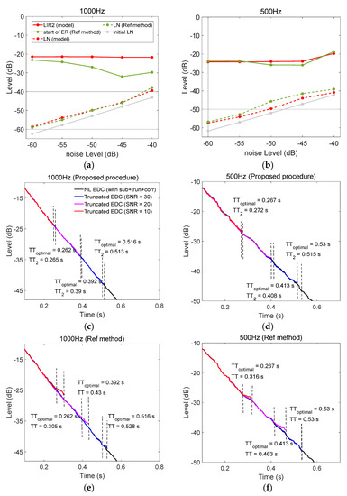
Figure 6.
Comparison of the results of the proposed procedure and the reference method with added pink noise (−60 dB to −40 dB) and band-pass filtering at the 1 kHz and 500 Hz: (a,b) The proposed procedure gives more stable parameters of LIR2 and LN. (c,d) Comparison of the truncated EDCs of the proposed procedure using the parameters in (a,b) from the reference NL EDC with the and (e,f) Comparison of the truncated EDCs of the reference procedure using the parameters in (a,b) from the reference NL EDC with the and .
Figure 6c,f presents the deviations of the truncated EDC of the proposed procedure and the reference method from the NL EDC. Figure 6e,f shows that in most cases, the reference method gives somewhat larger values of the than the of the proposed procedure. The truncated EDCs of the reference method have a certain deviation from the NL EDC between the detected and the optimal . The maximum deviation is approximately 2.4 dB, causing the relative error of the RT to be up to 8.4%. Section 4.1 illustrated that the deviation of the detected TT could be decreased by applying the correct safety margins.
Observing Figure 6c,d, the EDCs resulting from the proposed procedure show no truncation errors anymore. The truncated EDCs almost overlap the NL EDC above the detected . The error caused by the noise is reduced significantly when the noise level is −45 dB, causing a slight overestimation at 500 Hz. In this case, the maximum deviation is only 0.4 dB, resulting in the relative estimation error of RT being 2.1%. The slight shifts of the truncated EDCs from the NL EDC at the demonstrated that the procedure based on the double-slope decays model has good robustness to define an appropriate ER insensitivity to the noise fluctuation and the RIR irregularities.
5.2. TT Detection for Measured RIRs with Natural Ambient Noise
In the preceding sections, the proposed TT detection procedure was verified by its application on the measured RIRs with added noises that have double-slope decays. In this part, the proposed approach is applied to RIRs measured in rooms with real ambient noise. The reference RIRs having a high peak of the direct sound is measured with noise levels of −66.6 dB for room A and −56 dB for room B, and the noisy RIRs have noise levels of −50 dB and −46 dB, respectively. Figure 7 presents visual inspections of the EDCs fitting effects of the measured RIRs filtered in the octave bands generated from the model and the measured data. In the measured RIRs, the actual is generally unknown for noisy RIRs. Therefore, the analysis is to detect the using the proposed procedure, generating the truncated EDCs of the noisy RIRs filtered in the octave bands, and observing the deviations of these curves from the . The reference is obtained from the truncated EDCs of the reference RIRs using the reference method. The proposed procedure commonly used in practice is compared with the reference method introduced in Section 4.1. The is obtained from the truncated EDCs of the noisy RIRs by using the reference method. A detailed comparison of the RTs estimated at the and the between the truncated EDCs and the NL EDC proves that the process is effective in practical applications.
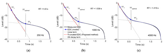
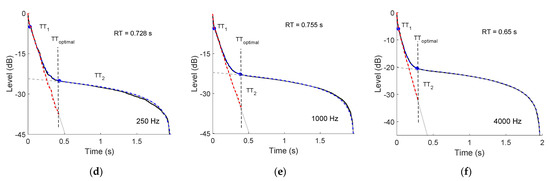
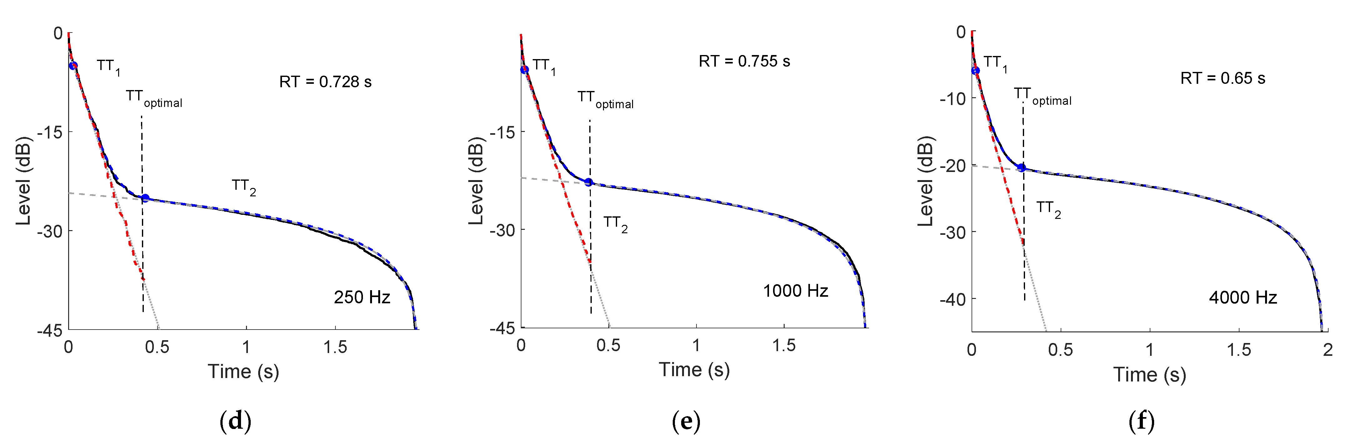
Figure 7.
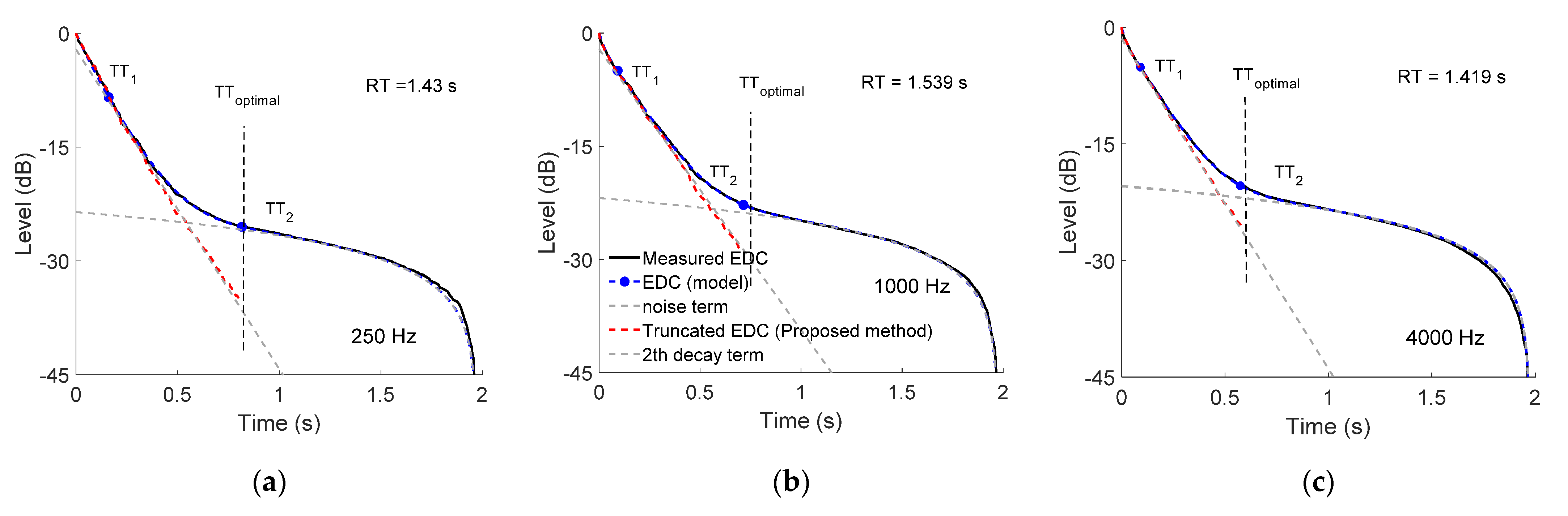
The normalized EDCs of the two measured RIRs having double-slope decays with ambient noise levels (−46 dB to −50 dB) filtered in the octave band at the 250 Hz, 1 kHz and 500 Hz, which generated from Equation (7), as well as the comparison of the corresponding to of the RIR with ambient noise levels (−56 dB to −66.6 dB).
Figure 7 presents the modeling of the EDCs generated for the measured RIRs filtered at 250 Hz, 1 kHz, and 4 kHz. The proposed procedure provides accurate parameters of the double-slope decays, and the ER of the start level and a noise level fully describe the EDCs of the measured data. The resulting logarithmic EDCs are almost identical to the measured EDCs. Table 2 presents the similar results of the DTs calculated from the RIRs with two different noise levels. The maximum relative difference of DT for room B was 0.26% at 1000 Hz. The maximum relative difference in the DT for room A was 2.19% at 125 Hz. The decay level differences of the EDCs between the proposed procedure and the measured EDC are relatively small above , with a maximum deviation of about 0.13 dB. Compared with RIRs with real ambient noise, the RIR with added pink noise shows slightly better fitting effects. The parameters in the model further define the ER of the noise compensation method to generate truncated EDCs (red dotted line) at the . Figure 7 shows that the second decay terms (gray dotted line) represent the decay slope of the EDC. The curves attach well with the truncated EDCs (red dotted lines).
Table 2.
Comparison of DTs between the measured RIRs with two noise levels.
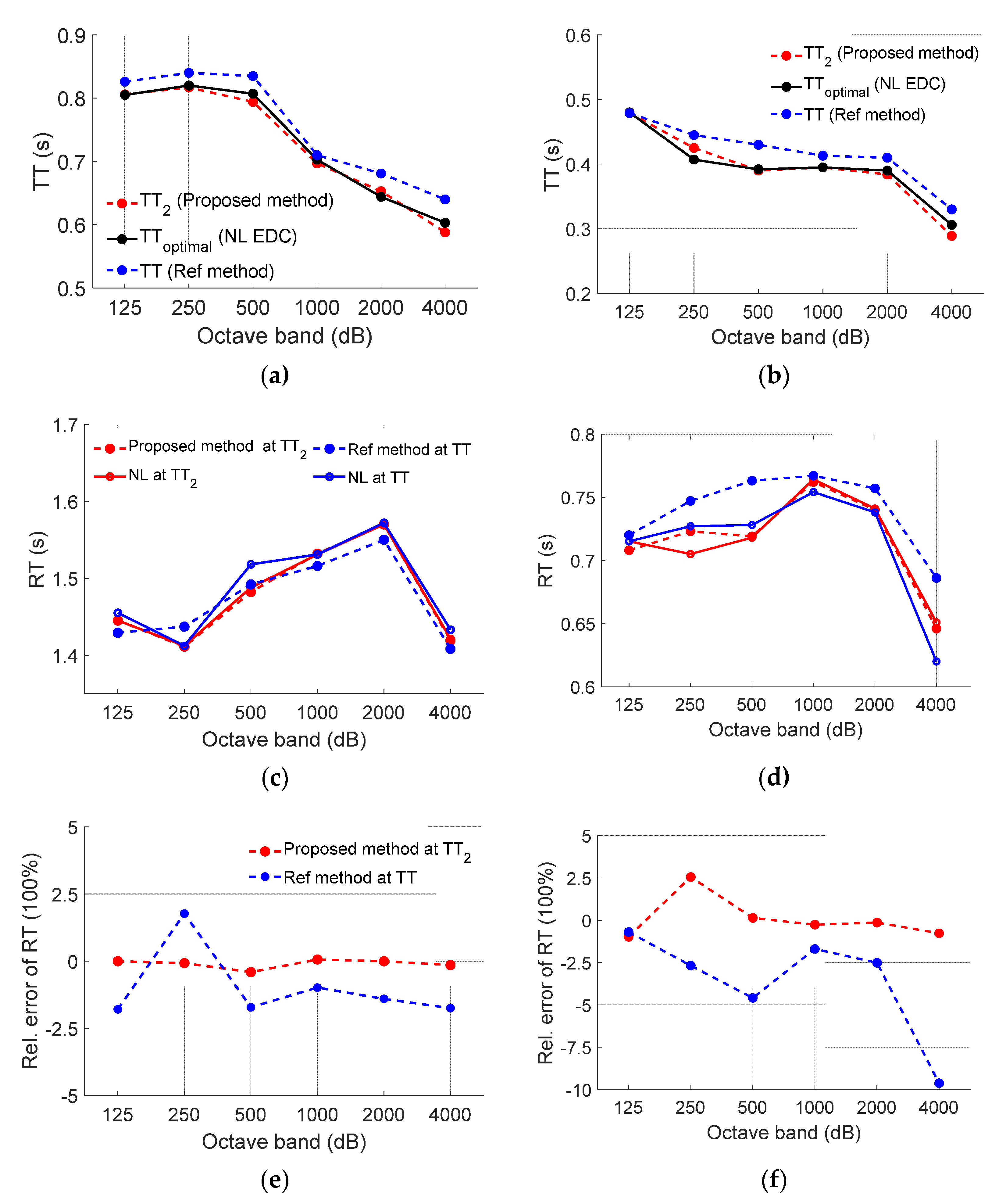
The and the RT of the reference method are taken as the reference results. As illustrated in Section 4.2, a certain deviation also appears at the truncated EDCs even if the RIR truncates at the actual TT. The deviations lead to the values in most octave bands shown in Figure 8a,b is larger than the . By comparing the RTs estimated from the truncated EDCs of the reference method at the to the RTs calculated from the NL EDC, the reference method leads to somewhat larger errors shown in Figure 8c,d. The relative errors of the estimated RTs are given in Figure 8e,f. The maximum relative errors of the RTs estimated at the were 9.62% for room A and 1.79% for room B. The deviations are approximately 2.9 dB and 0.4 dB.
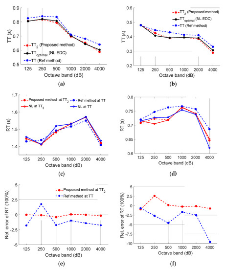
Figure 8.
Comparison of the proposed procedure and the compensation method for the RIR measured with ambient noise in two rooms and filtered in octave bands: (a,b) Comparison of the optimal TT of the NL EDC to the detected from the proposed method and the detected from the reference method. (c,d) Comparison of the corresponding RTs estimated at the and the located at the truncated EDCs and NL EDC. (e,f) Relative errors of the RTs.
The proposed method significantly reduces the truncation error, which leads to more stable results, yielding somewhat minor differences between the detected and the . The values of the are typically close to the , as shown in Figure 8a,b. The proposed method leads to similar maximum relative errors of the RTs estimated at the compared to the reference results, which were 2.55% for room A and 0.4% for room B. Compared to the , the maximum time difference of the is 75 ms while the value for is 17 ms. Furthermore, the deviation between the truncated EDC generated from the proposed method and the NL EDC at is relatively small, and it is less than 0.5 dB. However, the deviation of the between the truncated EDC of the reference method and the NL EDC is up to 1.8 dB. For the octave bands given in Figure 8e,f, the mean absolute values of the relative errors of RTs estimated at are 3.63% for room A and 1.56% for room B. The mean absolute values of the relative errors of RTs estimated at the are similar to that of the reference results. The mean absolute values are approximately 0.81% and 0.11%, respectively. Compared to the reference method, the proposed method provides a slightly better iterative procedure than the reference method since the proposed procedure enables the close to the optimal TT.
6. Conclusions
This study examines the possibility of combining a non-exponential decay model with the iterative procedure, which can fully automatically generate the close to the optimum. The model is represented by the parameters of double-slope decays, two decay levels for each decay term, and a stationary noise term. The parameter directly defines the start of the ER, and it can be calculated by the decay slope , and the LN. The parameter LN represents the end level of the ER. The proposed procedure decreases the influence of the RIR random fluctuations and the non-exponential decay behavior on the iterative procedure in the ER determination. This process automatically estimates the ER by iteratively minimizing the difference between the EDC of the model and the EDC generated from the RIR. The iterative procedure leads to convergence to the minimum value after several iterations after estimation of initial parameters by an LS optimization.
The process generates accurate parameters for the model, which can fully describe the EDCs of measured RIRs with double-slope decays and provide a more precise result of TT. The differences between the decay levels of the EDCs of the model Equation (6) and the reference RIR are minimized to a value less than 0.1 dB. In this case, the difference of the detected is approximately 0.009 s, resulting in the relative error of the corresponding RT being approximately 0.5%. The validity of the detected from the measured RIR with different noise levels was confirmed through analysis and comparison with the often-applied noise compensation method. The proposed procedure could be applied in a loop to exclude the influence of the curvature near the noise level and the high initial peaks of the RIR on the decay rate estimation, thus providing reliable model parameters of LN and . The truncated EDC resulting from the parameters show almost no truncation error anymore or a slight deviation at the , which is less than 0.5 dB in most cases. Compared with the reference noise compensation method, the proposed method provides a somewhat better iterative process for defining a TT that is more immune to the characteristic of the RIR.
Author Contributions
C.-M.L. gave academic guidance to this research work and revised the manuscript. M.C. designed the core methodology of this study, programmed the algorithms, carried out the experiments, and drafted the manuscript. Both authors have read and agreed to the published version of the manuscript.
Funding
This research received no external funding.
Institutional Review Board Statement
Not applicable.
Informed Consent Statement
Not applicable.
Data Availability Statement
Not applicable.
Conflicts of Interest
The authors declare no conflict of interest.
References
- ISO 140; Acoustics—Measurement of Sound Insulation in Buildings and of Building Elements. ISO: Geneva, Switzerland, 1998.
- ISO 354; Acoustics—Measurement of Sound Absorption in a Reverberation Room. ISO: Geneva, Switzerland, 2003.
- ISO 17497-1; Acoustics—Sound-Scattering Properties of Surfaces—Part 1: Measurement of the Random-Incidence Scattering Coefficient in a Reverberation Room. ISO: Geneva, Switzerland, 2006.
- Sant’Ana, D.Q.; Zannin, P.H.T. Acoustic evaluation of a contemporary church based on in situ measurements of reverberation time, definition, and computer-predicted speech transmission index. Build. Environ. 2011, 46, 511–517. [Google Scholar] [CrossRef]
- Cabrera, D.; Xuan, J.Y.; Guski, M. Calculating Reverberation Time from Impulse Responses: A Comparison of Software Implementations. Acoust. Aust. 2016, 44, 369–378. [Google Scholar] [CrossRef]
- Schroeder, M.R. New method of measuring reverberation time. J. Acoust. Soc. Am. 1965, 37, 409–412. [Google Scholar] [CrossRef]
- Morgan, D.R. A parametric error analysis of the backward integration method for reverberation time estimation. J. Acoust. Soc. Am. 1997, 101, 2686–2693. [Google Scholar] [CrossRef]
- Janković, M.; Ćirić, D.G.; Pantić, A. Automated estimation of the truncation of room impulse response by applying a nonlinear decay model. J. Acoust. Soc. Am. 2016, 139, 1047–1057. [Google Scholar] [CrossRef] [PubMed]
- ISO 3382–1:2009; Acoustics—Measurement of Room Acoustic Parameters—Part 1: Performance Spaces. ISO: Geneva, Switzerland, 2009.
- Lundeby, A.; Vigran, T.E.; Bietz, H.; Vorländer, M. Uncertainties of Measurements in Room Acoustics. Appl. Acoust. 1995, 81, 344–355. [Google Scholar]
- Chu, W.T. Comparison of Reverberation Measurements Using Schröder’s Impulse Method and Decay–Curve Averaging Method. J. Acoust. Soc. Am. 1998, 63, 1444–1450. [Google Scholar] [CrossRef] [Green Version]
- Christensen, C.L.; Koutsouris, G.; Rindel, J.H. The ISO 3382 parameters: Can we simulate them? Can we measure them? In Proceedings of the International Symposium on Room Acoustics, Toronto, ON, Canada, 9–11 June 2013; p. 10. [Google Scholar]
- Ćirić, D.G. Determination of truncation point of room impulse response. In Proceedings of the Forum Acusticum, Seville, Spain, 16–20 September 2002. [Google Scholar]
- Guski, M.; Vorländer, M. Comparison of noise compensation methods for room acoustic impulse response evaluations. Acta Acust. Acust. 2014, 100, 320–327. [Google Scholar] [CrossRef]
- Ćirić, D.G.; Makivirta, A.M. Optimal Determination of the Truncation Point of Room Impulse Responses. Building Acoust. 2005, 12, 15–30. [Google Scholar] [CrossRef]
- Ðorðe, M.D.; Ćirić, D.G.; Bratislav, B.P. De-Noising of a Room Impulse Response by Applying Wavelets. Acta Acust. United Acust. 2018, 104, 452–463. [Google Scholar]
- Ćirić, D.G.; Janković, M. Correction of room impulse response truncation based on a nonlinear decay model. Appl. Acoust. 2018, 132, 210–222. [Google Scholar] [CrossRef]
- Xiang, N. Architectural Acoustics Handbook; J. Ross Publishing: Plantation, FL, USA, 2017. [Google Scholar]
- Kuttruff, H. Coupled Rooms. Room Acoustics; E&FN Spon: London, UK, 2000; pp. 142–145. [Google Scholar]
- Xiang, N.; Goggans, P.M. Evaluation of decay times in coupled spaces: Bayesian parameter estimation. J. Acoust. Soc. Am. 2001, 110, 1415–1424. [Google Scholar] [CrossRef] [PubMed]
- Xiang, N.; Goggans, P.M.; Jasa, T.; Robinson, P. Bayesian characterization of multiple-slope sound energy decays in coupled-volume systems. J. Acoust. Soc. Am. 2011, 129, 741–752. [Google Scholar] [CrossRef] [PubMed] [Green Version]
- Chen, M.; Lee, C.M. De-Noising Process in Room Impulse Response with Generalized Spectral Subtraction. Appl. Sci. 2021, 11, 6858. [Google Scholar] [CrossRef]
- Matti, K.; Poju, A.; Aki, M. Estimation of Modal Decay Parameters from Noisy Response Measurements. J. Audio Eng. Soc. 2002, 11, 867–877. [Google Scholar]
- Jeong, D.; Joo, H. Prediction of reverberance in rooms with simulated non-single exponential sound decays. Appl. Acoust. 2017, 125, 136–146. [Google Scholar] [CrossRef]
- Hak, C.C.J.M.; Hak, J.P.M.; Wenmaekers, R.H.C. INR as an Estimator for the Decay Range of Room Acoustic Impulse Responses; AES Convention: Amsterdam, The Netherlands, 2008. [Google Scholar]
- Hak, C.C.J.M.; Wenmaekers, R.H.C.; Luxemburg, L.C.J.V. Measuring room impulse responses: Impact of the decay range on derived room acoustic parameters. Acta Acust. United Acust. 2012, 98, 907–915. [Google Scholar] [CrossRef] [Green Version]
- Xiang, N.; Sessler, G.M. Advanced Room-Acoustics Decay Analysis, in Acoustics, Information, and Communication; Xiang, N., Sessler, G., Eds.; Chapter 3; Springer: Cham, Switzerland; Heidelberg, Germany; New York, NY, USA; Dordrecht, The Netherlands; London, UK, 2015. [Google Scholar] [CrossRef]
- Xiang, N. Evaluation of reverberation times using a nonlinear regression approach. J. Acoust. Soc. Am. 1995, 98, 2112–2121. [Google Scholar] [CrossRef]
Publisher’s Note: MDPI stays neutral with regard to jurisdictional claims in published maps and institutional affiliations. |
© 2022 by the authors. Licensee MDPI, Basel, Switzerland. This article is an open access article distributed under the terms and conditions of the Creative Commons Attribution (CC BY) license (https://creativecommons.org/licenses/by/4.0/).