Article

Experimental Validation of the Model of Reverberation Time Prediction in a Room

by
Artur Nowoświat
* and
Marcelina Olechowska
Faculty of Civil Engineering, Silesian University of Technology, 44-100 Gliwice, Poland
*
Author to whom correspondence should be addressed.
Buildings 2022, 12(3), 347; https://doi.org/10.3390/buildings12030347
Submission received: 17 February 2022 / Revised: 6 March 2022 / Accepted: 10 March 2022 / Published: 13 March 2022
(This article belongs to the Special Issue Advances in Architectural Acoustics)

Abstract

:
It is well known that the uncertainty of input data has a great influence on the accuracy of room acoustics simulations. The aforementioned accuracy is significantly influenced by the selection of the acoustic properties of room-delimiting materials. Moreover, simulation errors are attributed to the fact that rooms can be very irregular and sound diffusion can be uneven, and thus sound absorption can be unevenly distributed over the surfaces. Therefore, a very important element is the validation of the simulation model of interior acoustics, even when we use ready-made software dedicated to interior acoustics for the simulation. In the article, the reverberation room model simulated in the ODEON program was subjected to validation. The program is based on a hybrid method combining the ray and virtual source methods. For the validation, appropriate measurements of the reverberation time in that room were carried out. The validation was undertaken using the criterion of correct validation, consisting of comparing the value of the comparison error and the value of the validation uncertainty.

1. Introduction

The acoustics of a room depends on the geometry, sound absorption or diffusivity of the acoustic field [1,2,3]. The acoustic properties of rooms are expressed by many different parameters, whose significance has been recognized by many researchers [4,5,6]. The most important parameter describing the interior acoustics is the reverberation time, which has a significant impact on other parameters used in this description [7,8]. Modern methods of design and acoustic adaptation of interiors are based on numerical methods [9]. Room acoustics can be simulated in two ways. The first one consists in solving the wave equation with the known solutions for rectangular rooms. For any room geometry, we apply the finite element method (FEM) [10,11], the finite-difference time-domain method (FDTD) [12,13] and the boundary element method (BEM) [14]. In the mid-low frequency range, especially when wave phenomena are strongly visible, wave methods are considered more accurate than geometric methods [15,16]. The BEM frequency domain is based on integral equations. This method is acknowledged because it is a convenient numerical tool for unlimited acoustic problems as its integral equation inherently satisfies the Sommerfeld radiation condition [17]. The fast multipole method (FMM) enables BEM to handle large acoustic models at high frequencies. This allows one to efficiently solve large limited problems, such as those of room acoustics [18]. In addition, FDTD, as a classic simulation method in the time domain, has good potential in a wide range of acoustic applications, including room acoustic simulations [19]. Yet, it is not certain that, given the complexity of the algorithms and numerical uncertainties, wave methods provide the best results. These techniques are expensive in terms of computation, especially in the range of medium and high frequencies, and they require knowledge of boundary surfaces of rooms, which is very often unavailable to the researcher (i.e., complex surface impedance). The second method, based on geometrical acoustics (GA) [20], is adopted for the frequency range above the Schroeder frequency in the room. The limitation of the GA method involves the fact it can be applied for medium and high frequencies for which the wavelength is small in relation to the dimensions of the room. Despite this, the geometric method is more computationally efficient compared to wave methods. Moreover, the problem of boundary conditions in the geometric method is reduced to the real coefficient of sound absorption by the material of the partitions delimiting the room. There are two main ways to model geometric acoustics: the ray-tracing method [21] and the image-source method [22]. In the simulation of room acoustics, diffuse reflection plays a very important role [23,24]. The modeling of room acoustics is approximated by hybrid approaches or the radiosity technique (the random-walk method) [25]. Various ways of implementing the GA algorithm can be distinguished, taking into account such aspects as: scattering coefficients [24], the choice of a transition point between two computation methods in hybrid algorithms [26] and the technique used to compute the diffuse reflections [27]. As a consequence, different algorithms provide different results when simulating the same room with identical input data [28,29]. The uncertainty of the final results of room acoustics modeling results from the uncertainty of many input parameters of the model, which should be identified and, if possible, reduced [9]. Computer simulations can be performed with ready-made software, e.g., ODEON [30,31]. Such simulation requires a three-dimensional room model that reflects the construction of the wall, floor and ceiling structures. For such a model, both sound absorption and reflection coefficients should be assigned to individual materials. At the design stage of new rooms, it is usually not difficult, because in simulations materials are used whose parameters are known from measurements or catalogs provided by manufacturers. However, at the stage of acoustic adaptation, the problem becomes significant, as most often the exact sound absorption or sound reflection coefficients of the materials present in the room are not known. That is why the validation of the numerical model is so important. In this article, such a validation was performed using laboratory measurements in a reverberation room. A model of such a reverberation room is presented, along with the measurement methodology and a validation method. The choice of this room was deliberate, because the purpose of this article is both to demonstrate the importance of validation and to test the “new” method of validation in interior acoustics. Only in laboratory conditions do we know both the acoustic absorption of the room and the behavior of the acoustic wave under various conditions of air humidity or air temperature.

2. Method

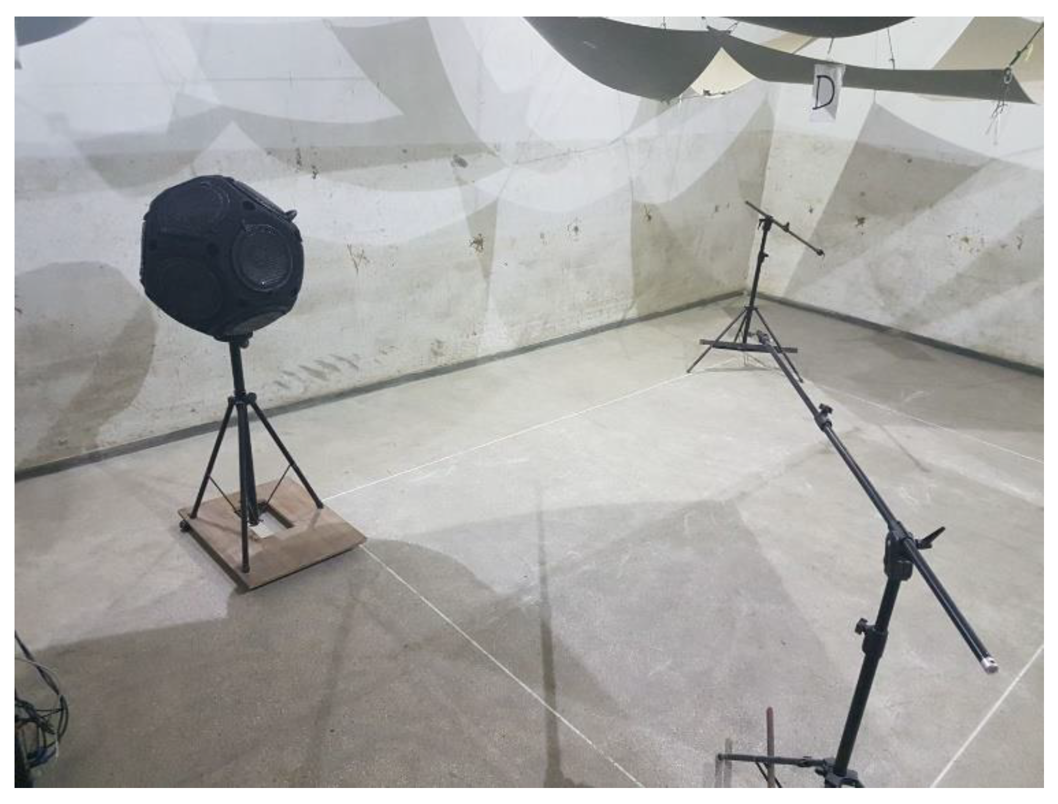
2.1. Measurement of Reverberation Time in a Reverberation Room

The measurements were taken in the reverberation room located in the acoustics laboratory at the Faculty of Civil Engineering of the Silesian University of Technology (Figure 1).
The volume of the reverberation room is 192.7 m3 [32] and its shape meets the requirements of the standard [33]:
l max < 1.9 V 1 3 ,
where:
  • lmax—the length of the longest straight line which fits within the boundary of the room (e.g., in a rectangular room it is the major diagonal), in meters,
  • V—the volume of the room, in cubic meters.
In the case of the described tests, the following was determined: l max = 9.12   m , 1.9 V 1 3 = 10.97   m . In order to ensure a diffused acoustic field, fixed, suspended diffusing elements were used. The microphones used for the measurement had omnidirectional characteristics, while the sound source had omnidirectional radiation characteristics. The measurements were made at two positions of the sound source. Six microphone settings were used for each source position. Six measurement repetitions were performed for each setting of the microphones. All combinations resulted in 12 spatially independent, measured sound decay curves. A total of 12 × 6 = 72 measurements were made. One of these systems is shown in Figure 2.
According to the standard [33], the positions of the microphones during the measurements were at least 1.5 m apart and at least 2 m from the sound source [34]. The measurements were made by the intermittent noise method. The transmission path consisted of a white and pink noise generator with an amplifier and a loudspeaker with spherical radiation characteristics. The receiving part consisted of an acoustic analyzer, microphones, pre-amplifier, acoustic calibrator and a computer with installed software.

2.2. Modeling

The ODEON software is a platform designed to simulate room acoustics. It applies a hybrid method using the algorithms of the ray method, image source method and energy method. For better understanding, the geometrical methods used in ODEON are presented.

2.2.1. Ray Method

In the ray method, a continuous acoustic wave is assumed to be a discrete set of sound rays that propagate at the speed of sound. These waves are emitted by the source and carry an equal part of the energy that is lost in subsequent reflections. The loss of this energy is proportional to the sound absorption coefficient of the boundary surface. When a wave hits a surface, it is reflected, which means that the new direction of wave propagation follows Snell’s law, which is known from geometric optics [35,36]. As the probability of hitting a specific point is close to zero, the receiving point is replaced with spatial elements, e.g., cones [37] or pyramids [38]. The energy drop due to the distance of the receiving point from the sound source is taken into account by the decrease in the number of rays reaching the point as the distance from the source increases. Thus, there is a risk of collecting false reflections and not catching the existing reflections. The ray may also hit the area A representing the receiving point after time t. This happens if the wave front represented by the ray is not larger than A/2. For this reason, the minimum number of rays N is estimated as:
N 8 π c 2 A t 2 ,
where c is the speed of sound in the room in m/s.
As a result, all energy-related data are averaged in the observation area, leading to the impulse response of the room in the time domain.

2.2.2. The Image Source Method

The image source method is considered to be a good approximation since the wavelength is short compared to the dimensions of the room. This means that it is suitable for simulating large spaces and high frequencies.
In this method, the geometrically determined mirror reflection of the acoustic wave is replaced by the reflection of the real sound source on the reflecting surface. On the extension of the direction of the ray reflected behind this plane, the virtual source is placed. The power of this source is equal to the power of the real source minus the energy losses resulting from the acoustic absorption of the partitions delimiting the room. On each reflecting surface real sources are distributed, which are the first order apparent sources. By mapping multiple reflections from all interior surfaces, higher order sources are generated. For subsequent reflections, the number of possible sources of images is [39]:
N s o u r c e s = 1 + n n 2 ( ( n 1 ) i 1 ) ( n 1 ) i ,
where:
  • n—the number of surfaces delimiting the room,
  • i—order of reflections of the sound wave.
Figure 3 shows the mirroring process, where S represents the source and I represents the mirror source. N denotes the normal to the surface, and ν is a vector from the source S to any point that lies on the surface, most commonly at any corner point. Thus, we can write [40]:
I = S 2 N | ν | cos α ,
In this method we set the termination condition, which can be set as the maximum order of reflections or maximum distance. Accordingly, the first order IS can be generated by mirroring the source S on all planes of the room. Then, for the second order reflections, all generated IS from the previous step must be mirrored on the surfaces of the room again. This process is repeated until the termination condition is met.

2.2.3. Hybrid Methods

The disadvantages of the ray method and the image source method have led to the development of hybrid models that combine the best features of these two methods [38,41]. The hybrid model uses the visibility test, which consists of tracing the rays from the source and recording the surfaces on which the rays fall. This method allows the elimination of the occurrence of rays representing the same sequences of sound waves reflections from the walls.

2.2.4. Computer Simulation Using ODEON

In the ODEON program, in the calculation algorithm, the “secondary sources” method was applied. After passing from the early reflections, the rays are treated as energy carriers and not as an element examining the geometry of the room. Each time a ray hits the surface, a secondary source is generated at the hit location. The energy generated in this secondary source is the total energy of the primary source divided by the number of rays and multiplied by the reflection coefficient of the surface on which it previously fell before reaching this secondary source. Each secondary source is a new sound source. Thus, the intensity of the new source is proportional to the cosine of the angle between the normal surface and the vector that starts at the secondary source point and ends at the new reception point. The reflection intensity at the reception point also decreases, in line with the inverse square law, at the beginning of the intensity vector in the starting point, which is the secondary source. Figure 4 shows schematically how the computational model behaves. Two adjacent rays are traced until the fifth reflection. From among all possible directions of reflection, one of them is chosen (randomly according to Lambert’s law). The next two reflections are specular and both rays find secondary sources S1 and S12. The rays of these sources generate one reflection. Rindel [39] determined that the optimal number of reflections is between 500 and 1000.
In the ODEON simulations, the scattering method was set to Lambert, and all directions of late reflections were calculated using the scattering coefficients. The sound source and receivers were placed at the same locations as during the measurements.
In the ODEON program, the geometry of the reverberation room and the positions of microphones and the sound source were mapped. The measurements and simulations were performed at a temperature of 15.5 °C and a relative humidity in the room of 30%. At the outset, the acoustic parameters of building partitions were selected, corresponding to a plastered and painted wall.

2.2.5. Validation

The following definition was adopted:
Definition 1.
Through the validation, the correctness of the model was assessed and adopted in relation to the results of the experimental tests.
In order to validate the model, the method proposed by Stern [42] was adapted.
Using Condition (5), the criterion of correct validation was described.
| E | < U V ,
where:
  • E—value of comparison error,
  • UV—validation uncertainty.
The validation error value was determined as follows:
E = δ E δ S ,
where:
  • δE—experimental error,
  • δS—simulation error.
δ S = δ S M A + δ S P D + δ S N ,
where:
  • δSMA—error resulting from the assumption of the model,
  • δSPD—error resulting from the use of input data.
  • δSN—error resulting from numerical simulation.
Based on the analysis of Formula (7) and taking into account the succeeding results of Stern et al. [43], it was concluded that the simulation error is very difficult to estimate for ready-made software such as ODEON. Therefore, a simpler method of its calculation has been proposed, expressed by the formula:
δ S = | S M | ,
where:
  • S—simulation result,
  • M—measurement result.
The value of validation uncertainty was defined as:
U V 2 = U E 2 + U S P E 2 + U S 2 ,
where:
  • UE—experimental uncertainty,
  • USPE—experimental uncertainty in the use of input data,
  • US—simulation uncertainty.

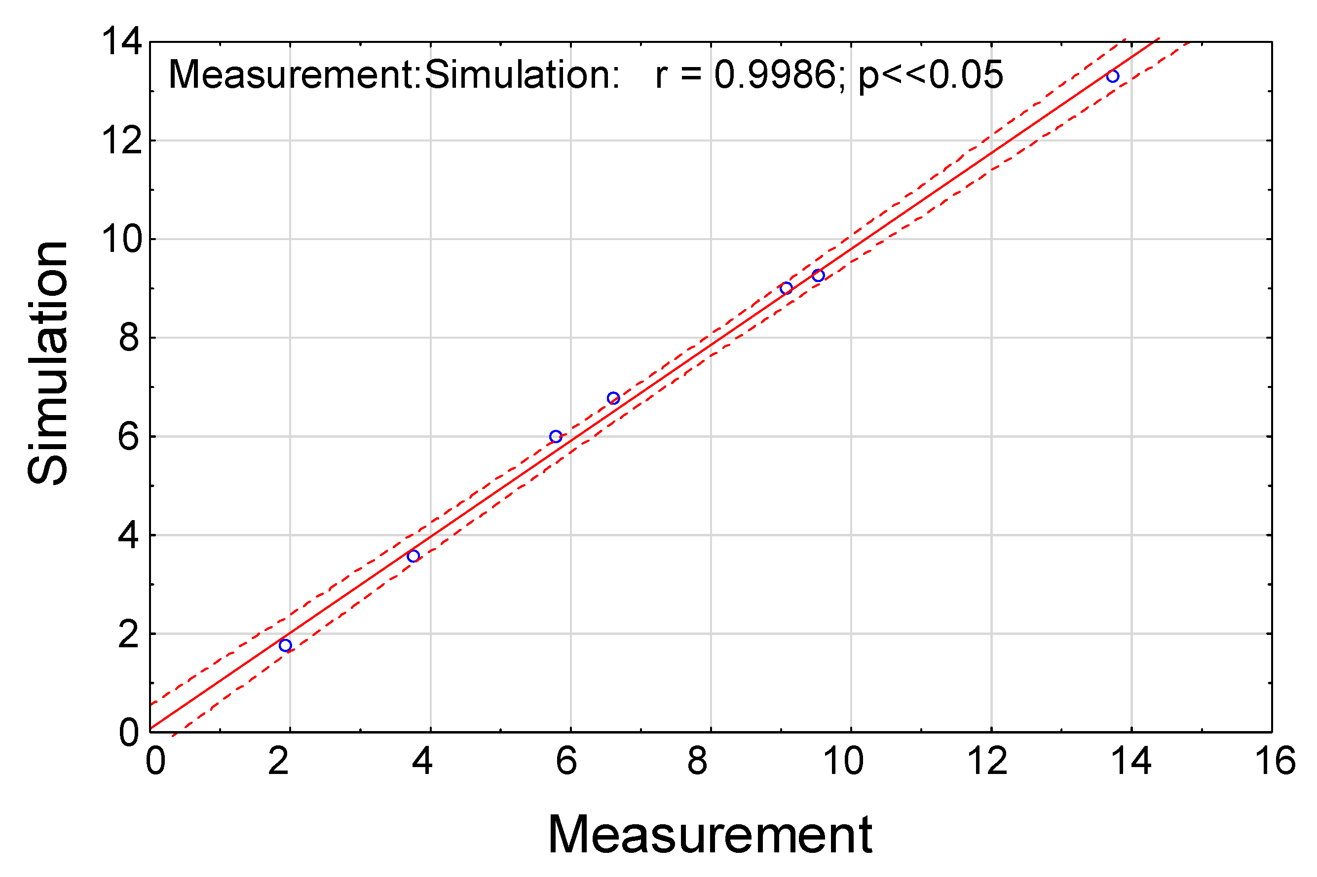
3. Results and Discussion

The acoustic absorption of the room was corrected in such a way as to ensure the conditions of good validation described by Formula (5).
Finally, the sound absorption coefficients of the walls as presented in Table 1 were adopted and compared with the tabular values for concrete.
In the first research step, the δS differences were determined using Dependence (8), and the results are presented in Table 2.
The mean relative error of the approximation of the reverberation times for the frequencies in the range of 63–4000 Hz is 4%. However, the relative error for the average reverberation time in the frequency range of 500, 1000 and 2000 Hz is 0.9%
The experimental error δE was adopted as an estimate of the mean standard deviation of the mean value, in line with the formula:
δ E = 1 n ( n 1 ) i = 1 n ( T ¯ T i ) 2 ,
where:
  • n—number of measurement samples,
  • Tii-th measurement of reverberation time,
  • T ¯ —arithmetic mean of all reverberation time measurements.
The statistical error in Equation (10) decreases with the rise in the number of samples, since under the law of large numbers, it tends to the constant value of the standard deviation of the random variable. The error resulting from the δS numerical simulation was accepted as the difference between the measured reverberation time and the simulated time. Without knowing the estimation error of the hybrid method, it would be difficult to estimate this error in a different way. However, taking into account that δS adopted in the described manner is the maximum error of the simulation, it should be stated that such an approach will at best overestimate this result. The results of the error values are summarized in Table 3.
The experimental uncertainty EU was adopted as the expanded uncertainty at the confidence level of 95%, which was expressed by the formula:
U E = U 95 ( T ¯ ) = k ( n ) δ E ,
where:
  • k(n)—extension value taking into account the student’s t distribution,
  • T ¯ —arithmetic mean of all reverberation time measurements.
In the present case k ( n ) = 1.96 .
Table 4 shows the uncertainty of the validation.
As can be seen from Table 3 and Table 4, Condition (5) is fulfilled for all frequency bands.
The fulfillment of the condition of good validation is confirmed by the presentation of the measurement and simulation results in one graph, as shown in Figure 5.
We have demonstrated that the condition of good validation has been met, and we confirm this condition graphically in Figure 5. However, we must add that the “proximity” of the measurement and simulation results is not enough to say that the simulation reflects the measurement result. If the measurement and simulation results fluctuated around each other, or if they were a product of randomness, we might not notice it. Therefore, in order to demonstrate, first, the high convergence of the results and, second, the statistical significance of the results, a correlation analysis was performed. The results of the analysis are presented in Figure 6.
As it can be observed, the correlation is at the level of r = 0.9986, which indicates a very high convergence of the results, and the test probability p << 0.05 indicates the statistical significance of the results. Thus, we conclude that the results are not accidental. However, the correlation alone is not enough to claim the similarity of results. The simulation and measurement results are identical when the regression line reflects the equation y = x. Therefore, the equation of the line shown in Figure 6 was determined:
S = 0.9729 M + 0.0754 ,
where:
  • S—simulation result,
  • M—measurement result.
As can be seen, the slope of the line is close to one and the shift along the vertical axis is very small.

4. Conclusions

The main goal was the demonstration of the validation of a numerical model. It was demonstrated that such a validation is also indispensable when using a ready-made computer program. Such a need arises mainly from the fact that errors occur when assigning certain values of sound absorption or sound diffusion to the partitions delimiting the room. For the purpose of validation, a method was proposed that consisted of comparing the value of the comparison error with the validation uncertainty. To ensure control over the model, the research was carried out in laboratory conditions in a reverberation room. It was found that the proposed method of validation was successful and it can be successfully used in the modeling of more complex rooms. In addition, the work describes the methods of acoustic geometry, which can be used when analyzing interior acoustics.
The following main conclusions can be drawn from the work:
  • the condition of the correct validation of Equation (5) known from the validation of proprietary numerical models works well during the modeling in ready-made software platforms when the input parameters are subject to high uncertainty;
  • the simulation error proposed by the authors with Formula (8) can be successfully used to validate numerical models in ready-made computer programs, when the input parameters are subject to high uncertainty;
  • the confirmation of the measurement reflected through simulation may be undertaken through regression analysis, where the regression equation y = x is interpreted as a very good (functional) representation.

Author Contributions

Conceptualization, A.N.; methodology, A.N.; software, M.O.; validation, A.N.; formal analysis, A.N.; investigation, A.N.; data curation, A.N. and M.O.; writing—original draft preparation, A.N.; writing—review and editing, A.N.; visualization, A.N. All authors have read and agreed to the published version of the manuscript.

Funding

This research received no external funding.

Institutional Review Board Statement

Not applicable.

Informed Consent Statement

Not applicable.

Data Availability Statement

The authors have all the data.

Conflicts of Interest

The authors declare no conflict of interest.

References

  1. Prędka, E.; Brański, A. Analysis of the room Acoustic with impedance boundary conditions in the full range of acoustic frequencies. Arch. Acoust. 2020, 45, 85–92. [Google Scholar]
  2. Nowoświat, A.; Olechowska, M.; Ślusarek, J. Prediction of reverberation time using the residual minimization method. Appl. Acoust. 2016, 106, 42–50. [Google Scholar] [CrossRef]
  3. Pilch, A.; Kamisiński, T. The effect of geometrical and material modification of sound diffusers on their acoustic parameters. Arch. Acoust. 2011, 36, 955–966. [Google Scholar] [CrossRef] [Green Version]
  4. Cerdá, S.; Gimènez, A.; Romero, J.; Cibrián, R.; Miralles, J.L. Room acoustical parameters: A factor analysis approach. Appl. Acoust. 2009, 70, 97–109. [Google Scholar] [CrossRef]
  5. Visentin, C.; Prodi, N.; Valau, V.; Picaut, J. A numerical and experimental validation of the room acoustics diffusion theory inside long rooms. In Proceedings of the 21st International Congress on Acoustics, Montreal, QC, Canada, 2–7 June 2013. [Google Scholar]
  6. Escobar, V.G.; Morillas, J.M. Analysis of intelligibility and reverberation time recommendations in educational rooms. Appl. Acoust. 2015, 96, 1–10. [Google Scholar] [CrossRef]
  7. Galbrun, L.; Kitapci, K. Accuracy of speech transmission index predictions based on the reverberation time and signal-to-noise ration. Appl. Acoust. 2014, 81, 1–14. [Google Scholar] [CrossRef]
  8. Meissner, M. Acoustics of small rectangular rooms. Analytical and numerical determination of reverberation parameters. Appl. Acoust. 2017, 120, 111–119. [Google Scholar] [CrossRef]
  9. Pilch, A. Optimization-based method for the calibration of geometrical acoustic models. Appl. Acoust. 2020, 170, 107495. [Google Scholar] [CrossRef]
  10. Magoules, F. (Ed.) Computional Methods for Acoustics Problems; Saxe-Coburg Publications: Stirling, UK, 2009. [Google Scholar]
  11. Atalla, N.; Sgard, F. Finite Element and Boundary Methods in Structural Acoustics and Vibration; CRC Press: Boca Raton, FL, USA, 2015. [Google Scholar]
  12. Bilbao, S.; Ahrens, J.; Hamilton, B. Incorporating sources directivity in wave-based virtual acoustics: Time-domain models and fitting to measured data. J. Acoust. Soc. Am. 2019, 146, 2692–2703. [Google Scholar] [CrossRef]
  13. Sakuma, T.; Sakamoto, S.; Otsuru, T. Computional Simulation in Architectural and Environmental Acoustics; Springer: Tokyo, Japan, 2014. [Google Scholar]
  14. Hargreaves, J.A.; Rendell, L.R.; Lam, Y.W. A framework for auralization of boundary element method simulations including source and receiver directivity. J. Acoust. Soc. Am. 2019, 145, 2625–2637. [Google Scholar] [CrossRef] [Green Version]
  15. Thydal, T.; Pind, F.; Jeong, C.H.; Emgsig-Karup, A.P. Experimental validation and uncertainty quantification in wave-based computational room acoustics. Appl. Acoust. 2021, 178, 107939. [Google Scholar] [CrossRef]
  16. Li, Y.; Meyer, J.; Lokki, T.; Cuenca, J.; Atak, O.; Desmet, W. Benchmarking of finite-difference time-domain method and fast multipole boundary element method for room acoustics. Appl. Acoust. 2022, 191, 108662. [Google Scholar] [CrossRef]
  17. Kirkup, S. The boundary element method in acoustics: A survey. Appl. Sci. 2019, 9, 1642. [Google Scholar] [CrossRef] [Green Version]
  18. Gumerov, N.A.; Duraiswami, R. Fast multipole accelerated boundary element methods for room acoustics. J. Acoust. Soc. Am. 2021, 150, 1707–1720. [Google Scholar] [CrossRef] [PubMed]
  19. Pelzer, S.; Aspöck, L.; Schröder, D.; Vorlönder, M. Integrating real-time room acoustics simulation into a CAD modeling software to enhance the architectural design process. Buildings 2014, 4, 113–138. [Google Scholar] [CrossRef]
  20. Savioja, L.; Svensson, U.P. Overwiew of geometrical room acoustic modeling techniques. J. Acoust. Soc. Am. 2015, 138, 708–730. [Google Scholar] [CrossRef] [Green Version]
  21. Winkler-Skalna, A.; Nowoświat, A. Use n-perturbation interval ray tracing method in predicting acoustic field distribution. Appl. Math. Model. 2021, 93, 426–442. [Google Scholar] [CrossRef]
  22. Panahi, E.; Younesian, D. Acoustic performance enhancement in a railway passenger carriage using hybrid ray-tracing and image-source method. Appl. Acoust. 2020, 170, 107527. [Google Scholar] [CrossRef]
  23. D’Antonio, P.; Cox, T.J. Diffusor application in rooms. Appl. Acoust. 2000, 60, 113–142. [Google Scholar] [CrossRef]
  24. Cox, T.J.; D’Antonio, P.; Vorlaender, M. A tutorial on scattering and diffusion coefficients for room acoustic surfaces. Acta Acoust. Acust. 2006, 92, 1–15. [Google Scholar]
  25. Tenenbaum, R.A.; Camilo, T.S.; Torres, J.C.B.; Gerges, S.N.Y. Hybrid method for numerical simulation of room acoustics: Part 1-theoretical and numerical aspects. J. Braz. Soc. Mech. Sci. Eng. 2007, 29, 211–221. [Google Scholar] [CrossRef] [Green Version]
  26. Stephenson, U. Analytical derivation of a formula for the reduction of computation time by the voxel crossing technique used in room acoustical simulation. Appl. Acoust. 2006, 67, 959–981. [Google Scholar] [CrossRef]
  27. Noriega-Linares, J.E.; Navarr, J.M. On the relations of room acoustic diffusion over binaural loudness. In Proceedings of the Euro Regio, Porto, Portugal, 13–15 June 2016. [Google Scholar]
  28. Vorländer, M. Computer simulations in room acoustics: Concept and uncertainties. J. Acoust. Soc. Am. 2013, 133, 1203–1213. [Google Scholar] [CrossRef] [PubMed]
  29. Berndäo, E.; Santos, E.S.O.; Melo, V.S.G.; Tenenbaum, R.A.; Meareze, P.H. On the performance investigation of distinct algorithms for room acoustics simulation. Appl. Acoust. 2022, 187, 108484. [Google Scholar] [CrossRef]
  30. Passero, C.R.M.; Zannin, P.H.T. Statistical comparison of reverberation times measured by the integrated impulse response and interrupted noise method, computionally simulated with ODEON software, and calculated by Sabine, Eyring and Arau-Puchades’ formulas. Appl. Acoust. 2010, 71, 1204–1210. [Google Scholar] [CrossRef]
  31. Nowoświat, A.; Olechowska, M.; Marchacz, M. The effect of acoustical remedies changing the reverberation time for different frequencies in a dome used for worship: A case study. Appl. Acoust. 2020, 160, 107143. [Google Scholar] [CrossRef]
  32. Nowoświat, A.; Bochen, J.; Dulak, L.; Żuchowski, R. Study on sound absotption of road acoustic screens under simulated weathering. Arch. Acoust. 2018, 43, 323–337. [Google Scholar]
  33. ISO 354: 2003; Acoustics—Measurement of Sound Absorption in a Reverberation Room. ISO: Geneva, Switzerland, 2003.
  34. Nowoświat, A.; Bochen, J.; Dulak, L.; Żuchowski, R. Investigation studies involving sound absorbing parameters of roadside screen panels subjected to aging in simulated conditions. Appl. Acoust. 2016, 111, 8–15. [Google Scholar] [CrossRef]
  35. Hohenwarter, D.; Jelinek, F. Snell’s law of refrectaction and sound rays for a moving medium. J. Acoust. Soc. Am. 1999, 105, 1387. [Google Scholar] [CrossRef]
  36. Zeng, X.; Christensen, C.L.; Rindel, J.H. Practical methods to define scattering coefficients in a room acoustics computer model. Appl. Acoust. 2006, 67, 771–786. [Google Scholar] [CrossRef]
  37. Vian, J.P.; van Maercke, D. Calculation of the room impulse response using a Ray-Tracking Method. In Proceedings of the ICA Symposium on Acoustics and Theatre Planning for the Performing Arts, Vancouver, BC, Canada, 4–6 August 1986. [Google Scholar]
  38. Vorländer, M. Simulation of the transient and steady-state sound propagation in rooms using a new combined ray-tracing/image source algorithm. J. Acoust. Soc. Am. 1989, 86, 172–178. [Google Scholar] [CrossRef]
  39. Rindel, J.H. The use of computer modeling in room acoustics. J. Vibroeng. 2000, 3, 219–224. [Google Scholar]
  40. Gkanos, K.; Pind, F.; Sørensen, H.H.B.; Jeong, C.H. Comparison of aparallel implementation strategies for the image source method for real-time virtual acoustics. Appl. Acoust. 2021, 178, 108000. [Google Scholar] [CrossRef]
  41. Naylor, G.M. ODEON—Another hybrid room acoustical model. Appl. Acoust. 1993, 38, 131–143. [Google Scholar] [CrossRef]
  42. Stern, F.; Wilson, R.; Coleman, H.; Paterson, E.G. Comprehensive approach to verification and validation of CFD simulations—Part 1: Methodology and procedures. J. Fluids Eng. 2001, 123, 793–802. [Google Scholar] [CrossRef]
  43. Stern, F.; Wilson, R.; Shao, J. Quantitative V&V of CFD simulations and certification of CFD codes. Int. J. Numer. Methods Fluids 2006, 50, 1335–1355. [Google Scholar]
Figure 1. Reverberation room: (a) cross-section of the reverberation room, (b) reverberation room projection [31].
Buildings 12 00347 g001
Figure 2. Microphone system—the source during the reverberation time of the reverberation room.
Buildings 12 00347 g002
Figure 3. Mirroring process of source S to the surface, creating the imaged source I.
Buildings 12 00347 g003
Figure 4. Principle of a hybrid model.
Buildings 12 00347 g004
Figure 5. The results of the reverberation room measurement and simulation.
Buildings 12 00347 g005
Figure 6. Scatterplot with correlation analysis.
Buildings 12 00347 g006
Table 1. Adopted sound absorption coefficients of room delimiting partitions (column 2) and sound absorption coefficients of concrete (column 3). Computer simulation and the measurement of reverberation time in the reverberation chamber.
Frequency [Hz]Adopted Sound Absorption CoefficientsSound Absorption Coefficients of Concrete
630.0110.01
1250.0160.01
2500.0150.02
5000.020.02
10000.020.02
20000.0260.02
40000.030.05
Table 2. Computer simulation and reverberation time measurement in the reverberation chamber.
Frequency [Hz]Measurement [s]SimulationValidation Error (8)
6313.7513.290.46
1259.089.000.08
2509.539.260.27
5006.616.760.15
10005.85.990.19
20003.763.570.19
40001.941.760.18
average 500, 1000, 20005.395.440.05
Table 3. Validation parameters of the reverberation time T. Value of error.
Frequency [Hz]Parameters of Error [%]Value of Error [%]
δEδS | E |
635.743.342.4
1253.010.882.13
2501.922.830.91
5001.382.270.89
10000.983.282.3
20000.645.054.41
40000.599.288.69
Table 4. Validation parameters of reverberation time T. Error value.
Frequency [Hz]Uncertainty of Measurement
and Simulation [%]
Uncertainty [%]
UEUSUV
6311.263.3411.74
1255.900.885.96
2503.762.834.71
5002.702.273.53
10001.923.283.80
20001.255.055.20
40001.159.289.35
Publisher’s Note: MDPI stays neutral with regard to jurisdictional claims in published maps and institutional affiliations.

