Abstract
Regarding the effect of the initial geometric defect (IGD) on the static stability of single-layer reticulated shells, its distribution pattern and magnitude are the main concerns to researchers. However, the suitable selection of the initial geometric defect magnitude (IGDM) is still a controversial topic. Therefore, it is intended to study the determination of the proper IGDM based on the structure force state (SFS) and the defect coefficient. In order to find out a qualified IGDM, more than 5200 numerical cases are carried out for four types of commonly used single-layer reticulated shells with the span ranging from 40 to 70 m and the rise–span ratio from 1/4 to 1/7, within the random defect mode method, by taking both geometric and material nonlinearity into account. The results show that it is more feasible to set the L/500 as IGDM when evaluating the stability of the single-layer reticulated shell. In addition, an updated criterion to identify the SFS at the stability critical state (SCS) is developed.
1. Introduction
Highlights:
- An accurate calculation method for the stable critical load of the single-layer reticulated shell is proposed.
- Put forward the calculation formula to evaluate the structural force state at stable critical state.
- An updated criterion to identify the structural force state at the stability critical state is developed.
- The initial geometric defect magnitude is determined by the structural force state and the defect coefficient.
Due to the light weight, excellent mechanical properties and economic benefits, single-layer reticulated shells are widely used in long-span space structures [1,2]. In our previous study, the static stability of single-layer reticulated spherical shells with Kiewitt–Sunflower type was discussed [3], and the damage constitutive model for circular steel tube of reticulated shells was proposed [4,5]. However, because of the initial eccentricity of member, the initial bending of member [6,7], the installation deviation of the reticulated shell node [8], etc., the phenomenon that IGD occurs in single-layer reticulated shells is nearly inevitable. In the early documented work, it is demonstrated that the single-layer reticulated shell is quite sensitive to IGD [9,10,11,12]. For instance, even a small IGD may lead to a substantial reduction in bearing capacity of the structure [13,14,15,16]. SFS regard as one of the reflections of structure stability; the relationship between SFS and IGDM is required for further investigation. Zhu [17] discussed the non-linear buckling load of aluminum alloy reticulated shells with gusset joints, and the result showed that the non-linear buckling load is not highly associated with the bending strain energy ratio and the total strain energy. Shan [18] examined the effect of joint stiffness on the dynamic response of single-layer reticulated shells jointed with bolt–column join, and the joint with large stiffness displayed deep plastic development. In order to exhibit the SFS in essence and ensure the structure safety, it is essential to consider the IGD in the stability analysis of the single-layer reticulated shells.
The influence of IGD on the stability of single-layer latticed shells are primarily charactered from two aspects: the distribution and the magnitude of IGD. With respect to various numerical methods to calculate IGD distribution, the consistent imperfection mode method [19] and random defect modal method [20] are the most popular. In consistent imperfection mode method, the lowest buckling mode is used as the IGD distribution mode, and the stability critical load (SCL) of the structure can be obtained through one direct calculation. However, the SCL obtained by this approach may not be reliable. Within the random defect mode method, the IGD can be allocated stochastically on the reticulated shell structure. Using this strategy, the obtained SCL is more accurate [21,22], though this approach is more expensive. With respect to IGDM, it was adopted as a certain value in early work [23,24,25]. Until recent decades, it was suggested by the current standard [26] that IGDM should be related to the span of the structure and could be assigned as L/300 (L is the structural span). Moreover, He et al. [16] investigated the elastic and elastic–plastic stability of the single-layer inverted catenary cylindrical reticulated shell, then proposed that it is appropriate to assign IGDM as an amplitude of 1/300 of the structural span in terms of the stability research on latticed shells. A similar conclusion was presented by Liu et al. [27] Meanwhile, Cui [28] evaluated the critical load capacity for the global instability of a spherical latticed shell, the IGDM of L/300 exhibited the ability to prevent the rapid decrease in critical load factor for a range of values of maximum IGD. Xiong [29] carried out an elasto-plastic stability analysis of the K6 shell with six different IGDMs, and the result indicated that when the IGDM was larger than L/300, the ultimate buckling load of K6 shells tended to be stable. However, according to the standard [26] and refs. [16,27], the lowest buckling mode is employed as the IGD distribution mode. Therefore, the obtained SCL of the structure is usually not the most critical, which leads to inaccurate analysis results. Guo [30] carried out a stability analysis of a single-layer latticed shell and three type of suspen-dome, then assumed that the installation deviation arranging from L/500 to L/300 can be regarded as the maximum allowable defect value of the reticulated shell. Chen et al. [12] conducted an experimental measurement of IGD of a real reticulated shell and insisted that the designed value of L/300 for IGD appears to be somewhat conservative. Su [31] proposed a new type of joint with the angled slotted-in steel plates, and the numerical result illustrated that the amplitude of IGD larger than L/1000 led to a great loss of its ultimate bucking capacity. Shen and Chen [32] pointed out that if the IGDM is too large, the structure may become a distorted structure. As mentioned above, a further discussion on the identification of suitable IGDM is required.
This paper intends to select a more reasonable IGDM which is suitable for reticulated shells with a different type, span, and rise–span ratio. Based on the comprehensive consideration of the SFS, the influence of IGD on the structural stability and structural defect coefficient, we intend to suggest L/500 as a more feasible value for IGDM in the stability investigation of single-layer reticulated shells in this work. This paper is organized as follows: in Section 2, the governing equation and constitutive model are described. Meanwhile, the calculation procedure of the SCL and analysis method of a single-layer latticed shell is introduced. In Section 3, the numerical analysis is carried out. In Section 4, the stress of the single-layer reticulated shell is analyzed, and the force state of the members and the structure is defined. Then, an updated criterion to identify the SFS at the SCS is proposed, and it is applied to determine the suitable IGDM. Furthermore, the IGDM is characterized using the defect coefficient. The conclusions are drawn in Section 5, and the recommendations for future research and engineering practice are put forward in Section 6.
2. Material and Methods
2.1. The Governing Equation and Constitutive Model
2.1.1. The Governing Equation
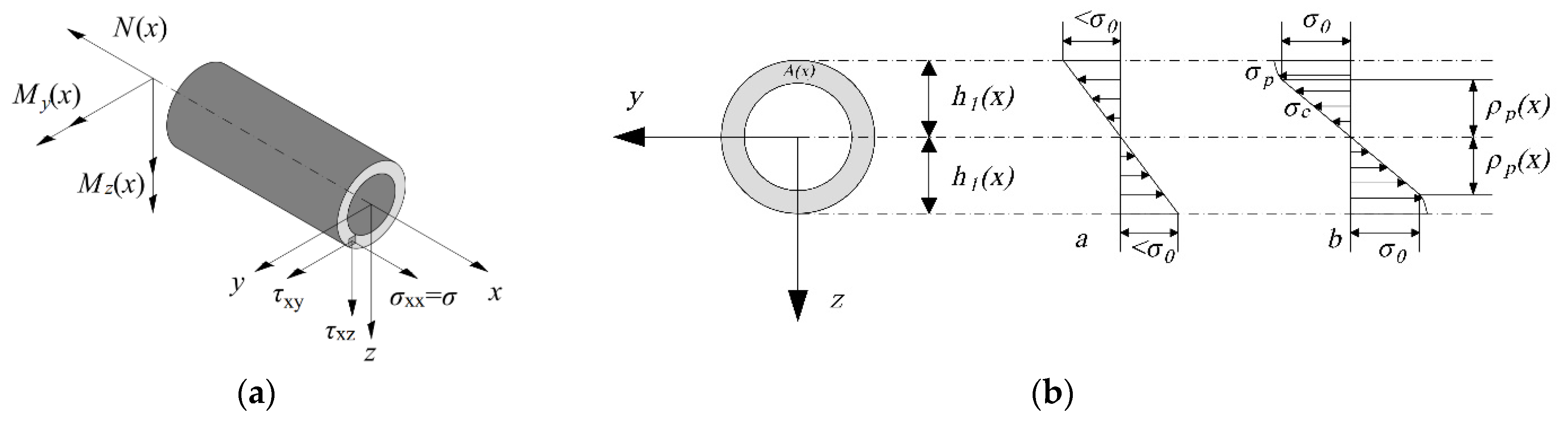
Motivated by the investigation on elastic–plastic bending of beams conducted by Štok and Halilovič [33], we assume that a straight circular steel tube with an area of cross section A(x) is mainly subjected to the bending moment My(x), Mz(x) and uniaxial force N(x), as shown in Figure 1a. As the tube studied in this work is slender (ratio l/D > 5, where l is the length of the tube and D is outer diameter for cross section), the shear stress is too small compared with the normal stress such that it can be ignored (i.e., τxy(x, y, z) = τxz(x, y, z) = 0). Then the governing equations of stress state distributed on the cross section can be identified according to the Bernoulli–Navier hypothesis on planarity and respective perpendicularity for cross section [34], which reads:

Figure 1.
Elastic and elastic–plastic stress distribution in a circular steel tube bending problem. (a): A straight circular steel tube subjected to the bending moment My(x), Mz(x), and uniaxial force N(x). (b): The stress distribution along the y and z directions.
Here, normal stress σ = σxx(x, y, z) is the sum of the stress caused by uniaxial force N(x), bending moments My(x) and Mz(x), respectively. The stress distribution along the y and z directions, for instance, is presented in Figure 1b, and it can be observed that before the stress achieves the yield stress σyield, the mechanical behavior is linear elastic, and it becomes nonlinear when the material comes to the plastic phase. Thus, the elastic–plastic response along the y direction can be expressed by the following:
where denotes the moment of inertia with respect to the y axis, δe indicates the elastic zone with the z direction and d is the inner diameter. σp is the plastic stress to be determined by our proposed constitutive model in the following section.
2.1.2. The Constitutive Model
According to the research over past decades, people have generally used the conventional Prandtl–Reuss material model, wherein the elastic–perfectly plastic stress–strain relations are derived on the basis of the von Mises yield criterion and its associated flow rule [35]. The Prandtl–Reuss model is the simplest ideal elasticity model. The material yield function adopts the Mises yield function, and its expression is
where J2 is the second stress tensor invariant, and k is the hardening coefficient. Then, the partial derivative of the yield function Φ with respect to the deviatoric stress tensor is written as
Furthermore, the variation of strain reads such that
where G indicates the shear modulus, K represents the bulk modulus, dλ is the plastic factor, and is the average of principal stress. Then, the variation of stress is denoted as
where we have
Thus, dλ, and can be written as follows:
2.2. Methodology
The analysis process on the static stability of the reticulated shell using the stochastic defect mode method is illustrated in Figure 2. The simulation is carried out based on the software ANSYS. It can be seen in Figure 2 that the finite element model of structure is established firstly. Then a reasonable initial geometric defect distribution pattern and magnitude are applied, and the appropriate numerical iterative calculation coefficients are set. The main factors to determine the convergence numerical method are the quality of grids, the reference arc length radius factor and the load steps. Since the grids are fixed once the finite element model is generated, if the numerical iteration is not convergent, the calculation coefficients involving the reference arc length radius factor and the load steps need to be adjusted until the solution satisfies the criterion. Finally, output the load-displacement result.
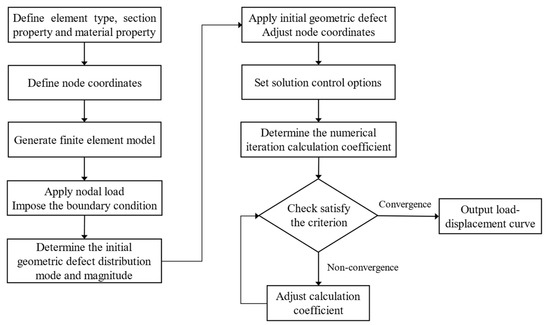
Figure 2.
The schematic diagram of static stability analysis for reticulated shell using stochastic defect mode method.
2.2.1. Analysis Model
For the analysis method, the complicated point is how to propose the hypothesis to impose the IGDM using the random defect mode method. In this work, two basic assumptions are adopted in the following:
- The installation deviation of each node in three directions of the coordinate axis conforms to the normal probability density function within the two-fold mean variance range, that is, the random variable of the installation deviation of each node is δX/2 (δ is the maximum allowable installation deviation, namely, the maximum calculated value of the initial geometric defect), and the random variable X obeys the standard normal distribution. The range of the error random variable is [−δ, δ];
- The random variable of each node installation error for the structure is mutually independent.
Based on the above assumptions, the installation deviation of each node of the structure is one multidimensional independent random variable, and each space sample point corresponds to one initial defect distribution pattern of the structure. Therefore, n samples can be taken out for nonlinear stability analysis, and the corresponding n SCL can be obtained.
In order to obtain the reasonable IGDM, it is essential to determine the SCL under the each IGDM. The calculation steps of the SCL of the reticulated shell within the random defect mode method are as follows:
- The installation deviation with random variable RW/2 is introduced for each node of calculation model (R is the maximum allowable installation deviation, and W is a random variable, which obeys the standard normal distribution). For each nonlinear buckling analysis of the model, a SCL can be obtained.
- After repeated calculation for n times, n sample space for SCL is generated.
- The SCL sample space follows the standard normal distribution, and hence the SCL of each model is determined by the “3σ” principle [36].
The SCL sample space capacity is set as n = 100.
2.2.2. Calculation Model
The difficulty of the calculation model is in computing the structural nonlinear stability during the development from the stable state to unstable state. It is required to study the equilibrium routine for the whole computation process. In this work, the arc-length method [37,38,39] is used to track the equilibrium path. The method is briefly introduced as follows. The linear finite element increment equation based on the energy variation principle can be expressed as
and employing the incremental displacement strategy proposed by Batoz and Dhatt [40], we can rewrite the Equation (16) by following
in which
where Kt is the structural tangential stiffness matrix at time t, ΔU(i) is the iteration displacement increment at current time step, F is the load vector, and is the proportional coefficient of load at the i-th iteration. There are N + 1 unknown ΔU(i) and Δλ(i) but only N linear equations above. Therefore, a constraint equation is demanded. For different types of arc-length methods, the constraint equations are different. Here, two kinds of constraint equations are presented, which read as follows:
- (1)
- Spherical arc-length method
- (2)
- Cylindrical arc-length methodwhere Δl is the increment of the arc length at each iteration.
The arc-length method uses an arc-length increment to determine the loading step, and the calculation is proceeded along the arc direction of the curve so that it is more adaptable than other methods. Regarding two arc-length methods referred above, the load increment method is used at the first calculation, and the structure displacement vector UΔt is obtained after iteration until it is convergent. Starting from the second step of the calculation, UΔt is substituted into Equations (21) or (22) to calculate the arc-length increment . The arc-length increment needs to be calculated before each computation, which yields the following:
where Δl is the arc length increment of the current computation step, N1 is the assumed optimal number of iterations at each step, and N2 is the number of iterations in the previous calculation step. Although the arc-length method is quite adaptable, it still has some limitations to some extent. It is suggested that adopting the iterative strategy flexibly and combining multiple methods reasonably is a good way to achieve an optimal balanced-path tracking.
2.2.3. Numerical Model
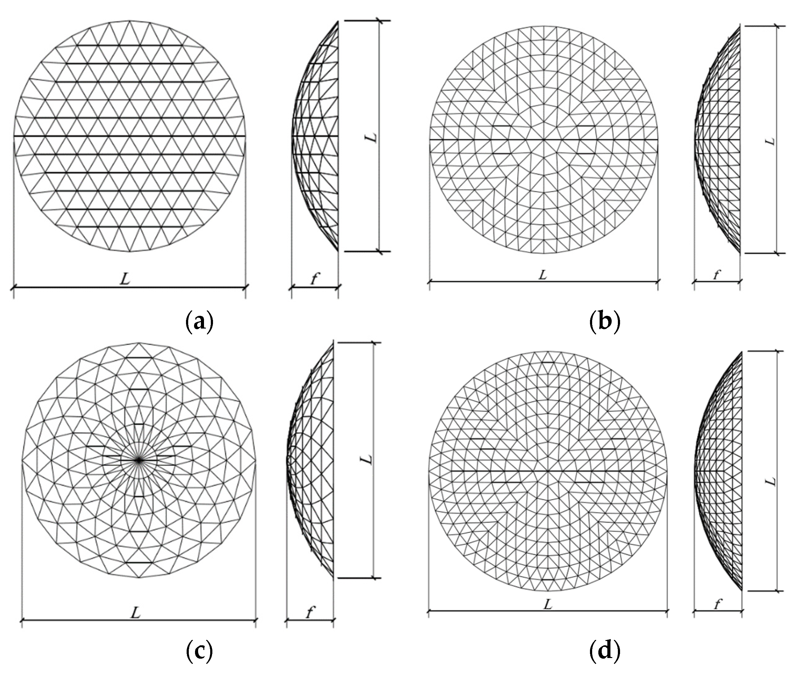
In the present paper, for the four types of commonly used, single-layer reticulated shells (as shown in Figure 3) are investigated through geometric and material nonlinear analysis within the random defect mode method, with the magnitude of δ = L/1000, L/900, L/800, L/700, L/600, L/500, L/400, L/300, L/200, and L/100 (δ is the IGDM). Parameters of single-layer reticulated shells are shown in Table 1. Steel with the elastic modulus E = 2.06 × 10⁶ MPa, the Poisson ratio ν = 0.3 and the yield strength fy = 240 MPa were determined as the material properties of calculation models. The roof static load is 0.8 kN/m2, and the roof live load, which is considered the whole span arrangement, is 0.5 kN/m2.
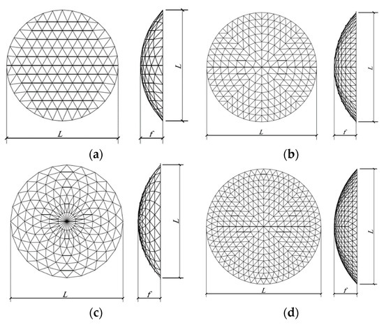
Figure 3.
The single-layer reticulated shell models. (a) Geodesic; (b) Kiewitt; (c) Sunflower; (d) Kiewitt 8-Sunflower.

Table 1.
Parameters of single-layer reticulated shells.
3. Results
In this paper, 4000 cases of elastic–plastic stability analysis were conducted. The numerical results of SCL were based on 100 cases and are presented in Table 2.
Table 2.
Maximum SCL under different IGDMs.
It is documented in the literature [32] that when the IGDM reaches L/300, the SCL falls to the minimum value. Then, with the increase in IGDM, the SCL performs an increase trend. Therefore, it is suggested in ref. [32] that the L/300 be regarded as the IGDM of the reticulated shell. Nevertheless, as it can be seen in Table 2, for all the models, with the increase in IGDM, the SCL always falls down, even until the end of calculation (δ = L/100). It is clear that the obtained result in our work is different from that in ref. [32]. The reasons can be attributed to two points by the following. (1) The random imperfections modal method is adopted in our work, while the consistent mode imperfection method is employed in ref. [32]. (2) Only the geometric nonlinearity of the structure is considered in ref. [32], whereas this paper takes into account the geometric and material nonlinearity. According to previous research, due to the large span of the reticulated shell, the plastic response of the member quite affects the mechanical behavior of the structure. He et al. [16] shows that the elastic–plastic ultimate strength of the structure could be computed by taking into account a plastic influence coefficient of 0.60 on the basis of the elastic result. Liu et al. [27] demonstrated that the ultimate bearing capacity of the latticed shell that considers the influence of material nonlinearity can be determined by multiplying the result of the ultimate bearing capacity of the latticed shell that does not consider the material nonlinearity by a reduction factor of 0.742. Hence, in order to find out a qualified IGDM, the double nonlinearity of the structure is used to analyze the single-layer reticulated shell structure within the random defect mode method in this manuscript.
4. Discussion
4.1. Stress Analysis
It is well known that the latticed shell structure is developed from a thin shell structure. In the early stability analysis of the latticed shell structure, the “method of simulated shell” is used to transform the reticulated shell structure into a continuous shell structure, and then some approximate nonlinear methods are used to solve the SCL of the reticulated shell structure. Although the finite element method is widely used, the analysis method of the thin shell theory can clearly understand the force characteristics of the reticulated shell structure. The internal forces generated by external forces in the reticulated shell structure are divided into “film internal force” and “bending internal force”, which correspond to the “no-moment theory” and “moment theory” of the thin shell structure, respectively. It can be seen from the force analysis of the reticulated shell by adopting the bending moment theory and the non-bending moment theory that the film internal force mainly drives the axial stress, while the bending internal force mainly triggers the bending stress and shear stress (including the torsional shear stress and transverse shear stress). In the stability analysis of the single-layer reticulated shell, the increase in IGDM not only reduces the SCL of structure, but also changes the SFS at SCS. Although the accepted reticulated shell structure in actual engineering inevitably has initial geometric defects, it is controlled in a small range, and hence the SFS is still dominated by the film internal force at SCS. If excessive IGD is applied in the stability analysis of latticed shell, the SFS may not conform to its actual working state, and the structure stability cannot be truly reflected. Therefore, this section puts forward the calculation formula to judge the SFS at SCS.
4.1.1. Analysis of the Member Force State
The identification of the SFS at SCS needs to be based on the analysis of the member force state. In order to study the member force state at SCS, the ratio of normal stress produced by the bending moment and axial force (RBA) is defined as
where , and are the RBA, maximum bending stress and axial stress of the i-th member, respectively. It should be pointed out that since the torsional and transverse shear stress of the member are rather smaller than the axial and bending stress during stability analysis of reticulated shell, the RBA can be used to represent the member force state directly. In this manuscript, the member with RBA less than 0.50 is defined as the member in which the force caused by axial stress dominates (MAS); otherwise, it is the member with the force led by both axial stress and bending stress (MAB).
4.1.2. Analysis of the SFS
Based on the classification of the member force state, the SFS at SCS can be examined subsequently. As discussed above, the member of the latticed shell structure is either MAS or MAB. This paper defined the following variables to represent the percentage of MAS and MAB among all the effective members, which read
where , and j are the average of the RBA of the MAS, sum of the RBA of the MAS, and number of the MAS, respectively, represents the percentage of MAS to effective member, , and k are the mean value of the RBA of the MAB, sum of the RBA of the MAB and number of the MAB, respectively, denotes the percentage of MAB to the effective member, and m is the number of effective members. As the bending stress and axial stress of the outermost ring member connected with the fixed hinge support are small, the value of RBA appears abnormal. Moreover, the outermost ring rod connected with the fixed hinge support has little influence on the overall buckling behavior of the structure. Therefore, when calculating the percentages of two kinds of members, the ring members at the support are not taken into account, which means the number of effective members. Meanwhile, m is computed by the difference between the number of all members and the number of outermost ring members.
The random defect mode method requires multiple calculations, and each calculation can produce a percentage of MAS and RBA of MAS. Therefore, the average of multiple calculations is applied by the following definitions:
where indicates the average of the MAS with RBA, represents the average percentage of MAS to effective member, expresses the average of the MAB with RBA, and denotes the average of percentage of MAB to effective member. Hence, the SFS is determined by the average of percentage of MAS to effective member and the average of RBA.
4.2. Selection of IGDM Based on the SFS
4.2.1. Determination Criteria for SFS
This section uses the same calculation model (four types of commonly used single-layer reticulated shells) as those in Section 2.2.2 to analyze the SFS under the SCS. The SFS under different IGDMs are shown in Table 3.
Table 3.
The SFS under different IGDMs.
It is clear in Table 3 that when the IGDM is less than L/500, with the increase in the IGDM, the decrease in the MAS with percentage and the increase in the MAS with RBA are slow. While after the IGDM is greater than L/500, with the increase in the IGDM, the drop of the MAS with percentage and the rise in the MAS with RBA are sharp. It indicates that with the rise in the IGDM, the SFS at SCS changes from the film internal force to the bending internal force. In this paper, the dual-control principle is proposed to judge the SFS at the SCS. To be specific, when the average of the percentage of MAS to the effective member is larger than 0.70, and meanwhile, in these members, the average of RBA is not larger than 0.25, and the SFS is dominated by the film internal force. As it is mentioned in Section 4.1, the SFS of the reticulated shell can be interpreted to be dominated by either the internal film force or bending moment, depending on the percentage of the MAS member (namely, the value of θN in Equation (30)). When considering the allowed IGDM for the reticulated shell in practical engineering, it is safe to control the SFS of the structure to perform as an internal film force. As it is illustrated in Table 3, before the IGDM δ reaches the L/500, the θN for all the four types of reticulated shell structures (Geodesic, Kiewitt 8, Sunflower, and K8-Sunflower) decreases steadily and the value of it remains beyond 70%. After that, the value of θN drops remarkably with the rise in IGDM δ, and its value falls beneath 50%, and to 20% finally. This means that the SFS of the shell structure changes to be dominated by the bending moment.
4.2.2. Determination of the IGDM
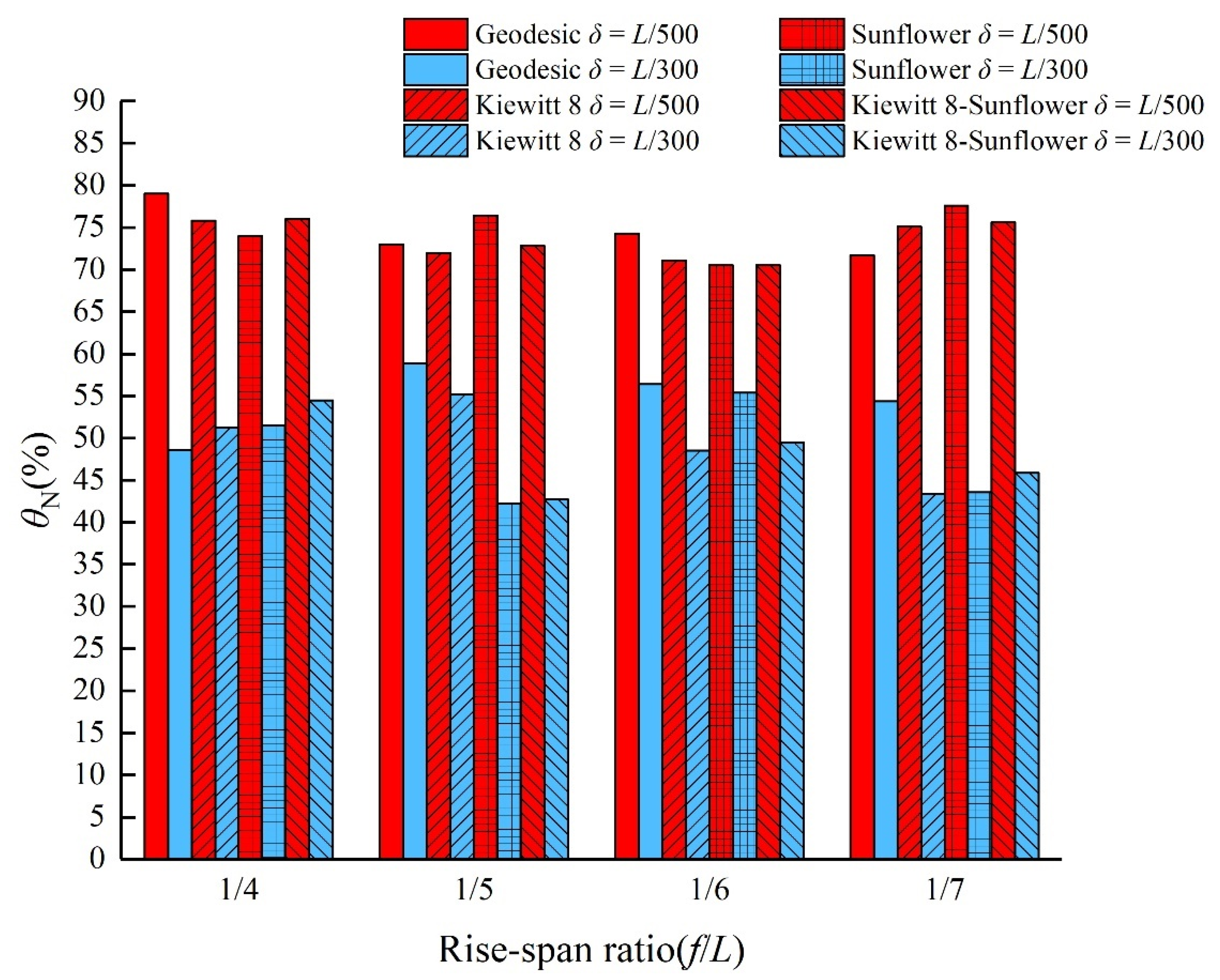
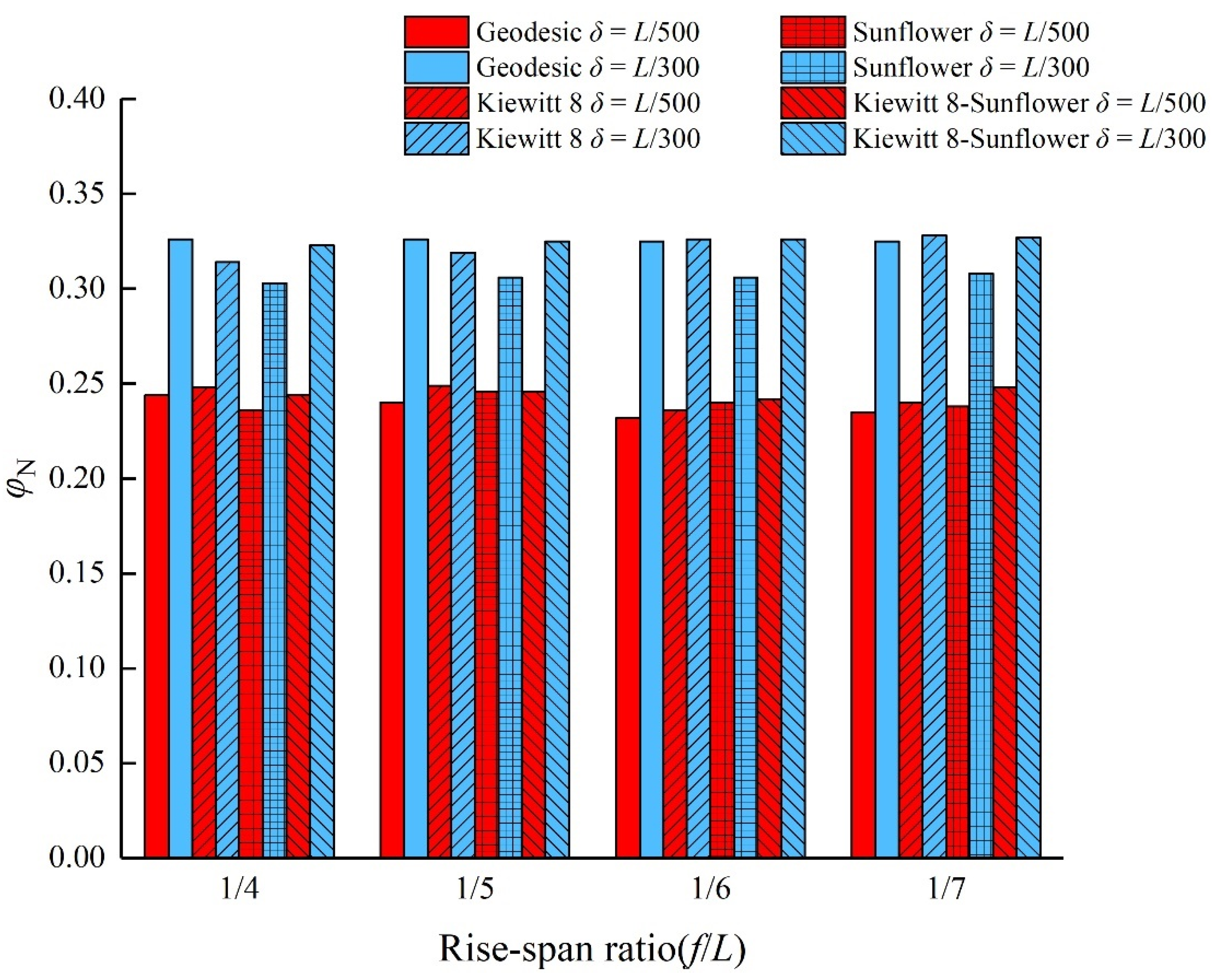
In this section, the value of IGDM is allocated as L/500 and L/300, respectively, which aims to figure out the effect of IGDM on the SFS at the critical situation. Four types of single-layer reticulated shells (Geodesic L = 40 m, Kiewitt 8 L = 50 m, Sunflower L = 60 m and Kiewitt 8-Sunflower L = 70 m) with a rise–span ratio (f/L = 1/4, 1/5, 1/6 and 1/7) are investigated within the random defect mode method and the 100 samples (n = 100). The SFS under the IGDM with L/500 and L/300 are reported in Table 4. The average of the percentage of MAS and the average of RBA of MAS are presented in Figure 4 and Figure 5, respectively.
Table 4.
The SFS under the IGDM with L/500 and L/300.
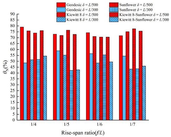
Figure 4.
The average of percentage of MAS with L/300 and L/500.

Figure 5.
The average of RBA of MAS with L/300 and L/500.
For each model, when the IGDM is L/500, the average of the percentage of MAS is over 70%, and the average of RBA is less than 0.25. It demonstrates that the film internal force is the main SFS. For each model, when the IGDM rises to L/300, the average of the percentage of MAS is less than 50%, and the average of RBA is greater than 0.30. It denotes that the SFS at SCS changes from the film internal force to the bending internal force (from Figure 4 and Figure 5). Therefore, it can be concluded that it is more reasonable to take the IGDM as L/500 in the stability analysis of the single-layer reticulated shell.
4.3. Selection of the IGDM Based on the Defect Coefficient
4.3.1. Choosing of the Defect Coefficient
To some extent, the IGD determines the SCL of the structure. In order to quantify this effect, this paper introduced a defect factor βδ to represent the decreasing amplitude of SCL on the latticed shell structure, which is expressed as follows:
where δ is the IGDM, and and are the SCL of imperfected and perfect structures, respectively. In this paper, the defect coefficient βδ is utilized to help to identify the IGDM. As we can see in Figure 6, for each structure, βδ can clearly reflect the influence of IGD on the SCL. It was suggested by Shen and Chen [32] and Fan et al. [9] that 50% of the SCL of the perfect lattice shell should be defined as the SCL of the defected latticed shell. It was proposed in ref. [16] that the ultimate bearing capacity of the structure with considering the geometric imperfection influence can be obtained through the perfect structure results multiplied by the reduction coefficient of 0.46. Therefore, it is appropriate to take the defect coefficient around 0.50. Note that the defect coefficient βδ defined in Equation 33 relies on the IGDM δ. As it is referred in Section 4.1 and Section 4.2.2, the primary factor to identify IGDM is to guarantee that the SFS of the shell mainly behaves as the internal film force, which is determined by the key parameter defined in Equation (30). Recall the definition of ; we find that it derives from the coefficient (RBA) in Equation (24). Look at the expression of in Equation (24); we recognize that it involves the performance of bending stress and axial stress , which is dependent on the material property. Hence, we assume that our defect model can be extended to different materials.
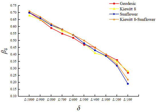
Figure 6.
The relationship between defect factor (βδ) and IGDM (δ).
As it is plotted in Figure 6, when the IGDM is L/1000, the defect coefficient βδ is about 70% for four kinds of reticulated shell structures, which means that the stability critical load (SCL) drops around 30%. With the increase in IGDM, the values of βδ decrease gradually with the nearly linear trend until the IGDM arrives L/300. Afterwards, the βδ falls sharply to a small magnitude finally (around 17% for the lowest value). This is because, as we mentioned in Section 4.2, as long as the IGDM is over L/300, the SFS transfer from the state is dominated by the internal film force to the situation controlled by the bending moment, which indicates that the shell structure is not so stable anymore, leading to the tremendous reduction in SCL. Therefore, in a word, it is assumed that the defect coefficient βδ is sensitive to IGDM δ in this work.
4.3.2. Identification of the IGDM
The same calculation model as those in Section 4.2.2 was used to figure out the feasible IGDM under the defect coefficient. The defect coefficient under the IGDM with L/300 and L/500 is shown in Table 5; when the IGDM is L/500, the defect coefficient of each model is around 0.48. As the IGDM increases to L/300, nearly all defect coefficients of the calculation model are less than 0.40. Thus, the selected IGDM is equal to L/500, which is more reasonable for the single-layer reticulated shell; meanwhile, it demonstrates that 0.50 as the defect coefficient is reasonable.
Table 5.
Defect coefficient under the IGDM with L/300 and L/500.
5. Conclusions
Based on four types of commonly used single-layer reticulated shells (Geodesic, Kiewitt 8, Sunflower, and Kiewitt 8-Sunflower), more than 5200 numerical cases of the elastic–plastic load-displacement of single-layer reticulated shells were investigated within the random defect mode method. Afterwards, an updated criterion to identify the structure force state at the stability critical state (SCS) was developed, and the reasonable initial geometric defect magnitude (IGDM) in the stability analysis of the single-layer reticulated shell was discussed. The main conclusions can be drawn as follows:
- Increasing the initial geometric defect magnitude (IGDM) within a rational range always leads to a fall down of the stability critical load (SCL), and it does not perform a smooth or increase trend as did the earlier research [32].
- It is feasible to select 0.50 as the defect coefficient, which is better to describe the influence of the initial geometric defect (IGD) on the structural stability.
- The structure force state at the stability critical state (SCS) could be estimated by the ratio of normal stress produced by the bending moment and axial force. Briefly speaking, when the average of percentage of the member in which the force caused by the axial stress dominates (MAS) and is larger than 0.70 and meanwhile in these members, the average of the ratio of normal stress produced by the bending moment and axial force (RBA) is less than 0.25, the structural force state is dominated by the film internal force.
- When the initial geometric defect magnitude (IGDM) is adopted as L/300, the structure force state (SFS) is not the film internal force, and hence in this case, the initial geometric defect (IGD) on the structural stability is overestimated. Therefore, considering the structure force state (SFS) and the influence of the initial geometric defect (IGD) on the structural stability, it is more proper to select L/500 as the initial geometric defect magnitude (IGDM).
6. Recommendation for Future Research and Engineering Practice
Future research in static stability analysis for reticulated shells is required to consider the influence of more parameters, including the initial geometric defect of the bar member, the semi-rigid connection, etc.
It is more reasonable to appropriately relax the requirement of the construction acceptance in the maximum coefficient of the initial geometric defect. The defect coefficient with 0.50 is recommended.
Author Contributions
Conceptualization, S.H. and P.Y.; methodology, S.H.; software, X.H. and W.Y.; validation, S.H., X.H. and W.Y.; formal analysis, S.H.; investigation, X.H. and W.Y.; resources, S.H.; data curation, X.H. and W.Y.; writing—original draft preparation, S.H.; writing—review and editing, P.Y.; visualization, X.H.; supervision, P.Y.; project administration, P.Y.; funding acquisition, S.H. and P.Y. All authors have read and agreed to the published version of the manuscript.
Funding
This study was funded by Guangxi Nature Science Foundation (2018JJB160052), Application of Key Technology in Building Construction of Prefabricated Steel Structure (BB30300105), Research Grant for 100 Talents of Guangxi Plan, Guangxi Key Research and Development Program (AB22036007), Guangxi Ba-Gui Scholars Program (2019A33), Guangxi Major Research Program (AB19259013).
Data Availability Statement
Some or all data, models, or code generated or used during the study are proprietary or confidential in nature and may only be provided with restrictions.
Conflicts of Interest
The authors declare that they have no conflict of interest.
Nomenclature
| IGD (Δ) | Initial Geometric Defect | R | Maximum allowable installation deviation |
| IGDM (δ) | Initial Geometric Defect Magnitude | W | Random variable |
| SFS | Structure Force State | Kt | Structural tangential stiffness matrix at time t |
| SCS | Stability Critical State | ΔU(i) | Iteration displacement increment at current time step |
| SCL | Stability Critical Load | F | Load vector |
| RBA (αi) | Ratio of normal stress produced by Bending moment and Axial force | Proportional coefficient of load at the i-th iteration | |
| MAS | Member in which the force caused by Axial Stress dominates | Δl | Increment of arc length at each iteration |
| MAB | Member with the force led by both Axial stress and Bending stress | N1 | Assumed optimal number of iterations at each step |
| L | Structural span | N2 | Number of iterations in the previous calculation step |
| A | Area of cross section of straight circular steel tube | E | Elastic modulus |
| My | Bending moment with y direction | ν | Poisson ratio |
| Mz | Bending moment with z direction | fy | Yield strength |
| N | Uniaxial force | f | Structural rise |
| l | Length of the tube | βδ | SCL ratio of the imperfect model to the perfect model |
| D | Outer diameter for cross section | σMi | Maximum bending stress |
| τxy | Shear stress with y direction | σNi | Axial stress of the i-th member |
| τxz | Shear stress with z direction | γN | Average of the RBA of the MAS |
| σxx | Normal stress | Sum of the RBA of the MAS | |
| σyield | Yield stress | j | Number of the MAS |
| Iy | Moment of inertia with respect to the y axis | ηN | Percentage of MAS to effective member |
| δe | Elastic zone with z direction | Mean value of the RBA of the MAB | |
| d | Inner diameter | Sum of the RBA of the MAB | |
| σp | Plastic stress | k | Number of the MAB |
| J2 | Second stress tensor invariant | Percentage of MAB to effective member | |
| k | Hardening coefficient | m | Number of effective members |
| Φ | Mises yield function | φN | Average of the MAS with RBA |
| Sij | Deviatoric stress tensor | θN | Average percentage of MAS to effective member |
| G | Shear modulus | Average of the MAB with RBA | |
| K | Bulk modulus | Average of percentage of MAB to effective member | |
| dλ | Plastic factor | Fδ | SCL of imperfected structure |
| σm | Average of principal stress | F0 | SCL of perfect structure |
| δσij | Variation of stress |
References
- Ma, J.; Fan, F.; Zhang, L.; Wu, C.; Zhi, X. Failure modes and failure mechanisms of single-layer reticulated domes subjected to interior blasts. Thin Wall Struct. 2018, 132, 208–216. [Google Scholar] [CrossRef]
- Fan, F.; Wang, D.; Zhi, X.; Shen, S. Failure modes of reticulated domes subjected to impact and the judgment. Thin Wall Struct. 2010, 48, 143–149. [Google Scholar] [CrossRef]
- Yu, P.; Yun, W.; Bordas, S.; He, S.; Zhou, Y. Static Stability Analysis of Single-Layer Reticulated Spherical Shell with Kiewitt-Sunflower Type. Int. J. Steel Struct. 2021, 21, 1859–1877. [Google Scholar] [CrossRef]
- He, S.; Wang, H.; Bordas, S.P.A.; Yu, P. A Developed Damage Constitutive Model for Circular Steel Tubes of Reticulated Shells. Int. J. Struct. Stab. Dyn. 2020, 20, 2050106. [Google Scholar] [CrossRef]
- He, S.; Nie, Y.; Bordas, S.P.A.; Yu, P. Damage-Plastic Constitutive Model of Thin-Walled Circular Steel Tubes for Space Structures. J. Eng. Mech. 2020, 146, 4020131. [Google Scholar] [CrossRef]
- Fan, F.; Yan, J.; Cao, Z. Elasto-plastic stability of single-layer reticulated domes with initial curvature of members. Thin Wall Struct. 2012, 60, 239–246. [Google Scholar] [CrossRef]
- Fan, F.; Yan, J.; Cao, Z. Stability of reticulated shells considering member buckling. J. Constr. Steel Res. 2012, 77, 32–42. [Google Scholar] [CrossRef]
- Zhao, Z.W.; Liu, H.Q.; Liang, B.; Yan, R.Z. Influence of random geometrical imperfection on the stability of single-layer reticulated domes with semi-rigid. Adv. Steel Constr. 2019, 15, 93–99. [Google Scholar] [CrossRef]
- Fan, F.; Cao, Z.; Shen, S. Elasto-plastic stability of single-layer reticulated shells. Thin Wall Struct. 2010, 48, 827–836. [Google Scholar] [CrossRef]
- Elishakoff, I. Uncertain buckling: Its past, present and future. Int. J. Solids Struct. 2000, 37, 6869–6889. [Google Scholar] [CrossRef]
- Bruno, L.; Sassone, M.; Venuti, F. Effects of the Equivalent Geometric Nodal Imperfections on the stability of single layer grid shells. Eng. Struct. 2016, 112, 184–199. [Google Scholar] [CrossRef] [Green Version]
- Chen, G.; Zhang, H.; Rasmussen, K.J.R.; Fan, F. Modeling geometric imperfections for reticulated shell structures using random field theory. Eng. Struct. 2016, 126, 481–489. [Google Scholar] [CrossRef]
- Kashani, M.; Croll, J.G.A. Lower bounds for overall buckling of spherical space domes. J. Eng. Mech. 1994, 120, 949–970. [Google Scholar] [CrossRef]
- Gioncu, V. Buckling of Reticulated Shells: State-of-the-Art. Int. J. Space Struct. 1995, 10, 1–46. [Google Scholar] [CrossRef]
- Kato, S.; Mutoh, I.; Shomura, M. Collapse of semi-rigidly jointed reticulated domes with initial geometric imperfections. J. Constr. Steel Res. 1998, 48, 145–168. [Google Scholar] [CrossRef]
- He, Y.; Zhou, X.; Liu, D. Research on stability of single-layer inverted catenary cylindrical reticulated shells. Thin Wall Struct. 2014, 82, 233–244. [Google Scholar] [CrossRef]
- Zhu, S.; Ohsaki, M.; Guo, X.; Zeng, Q. Shape optimization for non-linear buckling load of aluminum alloy reticulated shells with gusset joints. Thin Wall Struct. 2020, 154, 106830. [Google Scholar] [CrossRef]
- Shan, Z.; Ma, H.; Yu, Z.; Fan, F. Dynamic failure mechanism of single-layer reticulated (SLR) shells with bolt-column (BC) joint. J. Constr. Steel Res. 2020, 169, 106042. [Google Scholar] [CrossRef]
- Chen, X.; Shen, S.Z. Complete Load-Deflection Response and Initial Imperfection Analysis of Single-Layer Lattice Dome. Int. J. Space Struct. 1993, 8, 271–278. [Google Scholar] [CrossRef]
- Yamada, S.; Takeuchi, A.; Tada, Y.; Tsutsumi, K. Imperfection-sensitive overall buckling of single-layer lattice domes. J. Eng. Mech. 2001, 127, 382–386. [Google Scholar] [CrossRef]
- Zhao, J.; Zhang, Y.; Lin, Y. Study on mid-height horizontal bracing forces considering random initial geometric imperfections. J. Constr. Steel Res. 2014, 92, 55–66. [Google Scholar] [CrossRef]
- Liu, H.; Zhang, W.; Yuan, H. Structural stability analysis of single-layer reticulated shells with stochastic imperfections. Eng. Struct. 2016, 124, 473–479. [Google Scholar] [CrossRef]
- See, T.; McConnel, R.E. Large displacement elastic buckling of space structures. J. Struct. Eng. 1986, 112, 1052–1069. [Google Scholar] [CrossRef]
- Borri, C.; Spinelli, P. Buckling and post-buckling behaviour of single layer reticulated shells affected by random Buckling and post-buckling behaviour of single layer reticulated shells affected by random imperfections. Comput. Struct. 1988, 4, 937–943. [Google Scholar] [CrossRef]
- Morris, N.F. Effect of imperfections on lattice shells. J. Struct. Eng. 1991, 117, 1796–1814. [Google Scholar] [CrossRef]
- Ministry of Housing and Urban-Rural Development of the People’s Republic of China. Technical Specification for Space Frame Structure. (JGJ7–2010); China Architecture Industry Press: Beijing, China, 2010. [Google Scholar]
- Liu, H.; Ding, Y.; Chen, Z. Static stability behavior of aluminum alloy single-layer spherical latticed shell structure with Temcor joints. Thin Wall Struct. 2017, 120, 355–365. [Google Scholar] [CrossRef]
- Cui, X.Z.; Li, Y.G.; Hong, H.P. Effect of spatially correlated initial geometric imperfection on reliability of spherical latticed shell considering global instability. Struct. Saf. 2020, 82, 101895. [Google Scholar] [CrossRef]
- Xiong, Z.; Guo, X.; Luo, Y.; Zhu, S. Elasto-plastic stability of single-layer reticulated shells with aluminium alloy gusset joints. Thin Wall Struct. 2017, 115, 163–175. [Google Scholar] [CrossRef]
- Guo, J.M. Research on distribution and magnitude of initial geometrical imperfection affecting stability of suspen-dome. Adv. Steel Constr. 2011, 7, 344–358. [Google Scholar]
- Shu, Z.; Li, Z.; He, M.; Chen, F.; Hu, C.; Liang, F. Bolted joints for small and medium reticulated timber domes: Experimental study, numerical simulation, and design strength estimation. Arch. Civ. Mech. Eng. 2020, 20, 1–24. [Google Scholar] [CrossRef]
- Shen, S.Z.; Chen, X. Stability of Lattice Shell Structures; Science Press of China: Beijing, China, 1999. [Google Scholar]
- Štok, B.; Halilovič, M. Analytical solutions in elasto-plastic bending of beams with rectangular cross section. Appl. Math. Model. 2009, 33, 1749–1760. [Google Scholar] [CrossRef]
- Dai, H.H.; Huo, Y. Asymptotically approximate model equations for nonlinear dispersive waves in incompressible elastic rods. Acta Mech. 2002, 157, 97–112. [Google Scholar] [CrossRef]
- Chen, W.-F.; Han, D.-J. Plasticity for Structural Engineers; Springer Science & Business Media: Berlin, Germany, 2012. [Google Scholar]
- Rice, J.A. Mathematical Statistics and Data Analysis; Cengage Learning: Boston, MA, USA, 2006. [Google Scholar]
- Crisfield, M.A. A faster modified newton-raphson iteration. Comput. Methods Appl. Mech. Eng. 1979, 20, 267–278. [Google Scholar] [CrossRef]
- Crisfield, M.A. An arc-length method including line searches and accelerations. Int. J. Numer. Methods Eng. 1983, 19, 1269–1289. [Google Scholar] [CrossRef]
- Riks, E. An incremental approach to the solution of snapping and buckling problems. Int. J. Solids Struct. 1979, 15, 529–551. [Google Scholar] [CrossRef]
- Batoz, J.; Dhatt, G. Incremental displacement algorithms for nonlinear problems. Int. J. Numer. Methods Eng. 1979, 14, 1262–1267. [Google Scholar] [CrossRef]


Publisher’s Note: MDPI stays neutral with regard to jurisdictional claims in published maps and institutional affiliations. |
© 2022 by the authors. Licensee MDPI, Basel, Switzerland. This article is an open access article distributed under the terms and conditions of the Creative Commons Attribution (CC BY) license (https://creativecommons.org/licenses/by/4.0/).