Article

Prediction of Compaction and Strength Properties of Amended Soil Using Machine Learning

by
Woubishet Zewdu Taffese
1,* and
Kassahun Admassu Abegaz
2
1
Department of Civil Engineering, Aalto University, 02150 Espoo, Finland
2
Department of Construction Engineering and Management, Institute of Technology, University of Gondar, Gondar P.O. Box 385, Ethiopia
*
Author to whom correspondence should be addressed.
Buildings 2022, 12(5), 613; https://doi.org/10.3390/buildings12050613
Submission received: 7 April 2022 / Revised: 23 April 2022 / Accepted: 2 May 2022 / Published: 6 May 2022
(This article belongs to the Section Construction Management, and Computers & Digitization)

Abstract

:
In the current work, a systematic approach is exercised to monitor amended soil reliability for a housing development program to holistically understand the targeted material mixture and the building input derived, focusing on the three governing parameters: (i) optimum moisture content (OMC), (ii) maximum dry density (MDD), and (iii) unconfined compressive strength (UCS). It is in essence the selection of machine learning algorithms that could optimally show the true relation of these factors in the best possible way. Thus, among the machine learning approaches, the optimizable ensemble and artificial neural networks were focused on. The data sources were those compiled from wide-ranging literature sources distributed over the five continents and twelve countries of origin. After a rigorous manipulation, synthesis, and results analyses, it was found that the selected algorithms performed well to better approximate OMC and UCS, whereas that of the MDD result falls short of the established threshold of the set limits referring to the MSE statistical performance evaluation metrics.

1. Introduction

Chemical soil stabilization is the most common method, which involves adding chemical stabilizers (mainly cement and/or supplementary cementitious materials) to soils in order to improve their strength and durability properties [1,2,3]. This form of stabilization usually results in cost reductions when performing civil engineering works such as foundation and stabilized soil block production. Compaction is also another essential method for improving the engineering features of earth-based construction for controlling shrinkage and lowering permeability, resulting in a more stable structure [3]. For any soil type in earthworks, the OMC of the soil being compacted at which the MDD is obtained must be measured in order to obtain effective compaction in stabilization. Soil strength enhancing method, like compaction, is also critical to the design, construction, and long-term sustainability of earth-based structures.
It is prudent to develop models for predicting OMC, MDD, and UCS from the properties of natural soils and chemical stabilizers. This is due to the need to avoid extensive and time-consuming laboratory testing for the appropriate selection of a chemical stabilizer on every new project [4,5]. Indeed, because of the numerous and unclear physical processes involved in the formation of natural soils and stabilizers, their properties exhibit a wide range of responses to environmental impacts. Due to the intricacy of the natural soil behavior, as well as its spatial variability and the inclusion of stabilizers, developing physics-based prediction models for OMC, MDD, and UCS is complex. Unlike a physics-based system that follows explicit rules to complete a task, such a complex problem necessitates the use of systems that can learn from experience. Therefore, using machine learning algorithms is the best option as they are able to learn from data and solve complex problems without making assumptions.
Several machine learning algorithms have recently been used to predict OMC, MDD, and UCS of stabilized and natural soils. For instance, Ref. [6] proposed an artificial neural network (ANN) to predict MDD and OMC of stabilized soil. The architecture of the adopted ANN models was a multilayer perceptron (MLP), consisting of layers composed of neurons and their connections. The performance evaluation of the models demonstrated that they yield satisfactory results. Additionally, Ref. [7] tried to predict MDD and UCS of cement stabilized soils using three types of ANN methods and a support vector machine (SVM). The adopted ANN models are differential evolution, Bayesian regularization, and Levenberg–Marquardt. After considering the performance metrics, the authors concluded that the SVM is superior to the ANN-based models. Ref. [8] utilized adaptive neuro fuzzy inference system (ANFIS) and nonlinear regression (NLR) to predict the UCS of stabilized soil. The author compared the accuracy of an ANFIS-based UCS prediction model to that of nonlinear regression and concludes that the former is superior. The ANN and ANFIS methods have also been used to estimate the UCS of compacted soils [9]. The authors evaluated the effectiveness of the two models and discovered that the ANN is less superior to the ANFIS. Machine learning models were developed by [10] to predict the UCS and MDD of soils stabilized by cement. The adopted machine learning algorithms were multivariate adaptive regression splines and functional networks, and their performance was compared to four models presented in [7], namely SVM and ANN (Bayesian regularization, differential evolution, and Levenberg–Marquardt). Based on statistical performance measurements, the authors claimed that the algorithms used outperform ANN and SVM-based models. According to [11], ANN can be used to accurately predict UCS fiber reinforced cement stabilized fly ash mixes. The authors also evaluated by comparing its performance to that of the traditional multiple linear regression model and concluded that it is inferior to the ANN. ANN was used by [2] to predict the MDD and OMC of clayey soils stabilized by lime. According to the authors, the developed ANN model can accurately predict both properties of the stabilized soils [12] and also utilized ANN to build a model predicting soil UCS. The study concluded that ANN could predict UCS with high accuracy.
The preceding works, which attempted to predict OMC, MDD, and UCS of stabilized soils by applying machine learning methods, are exhilarating. However, most of the adopted algorithms are single ones which may not make the optimal prediction for a given dataset. Among all single algorithms, ANN is the most employed one, but ANN failed to examine its prediction performance with different types of backpropagation algorithms. The utilization of ensemble methods, which is a machine learning technique that combines several base models, is the best alternative approach to produce an optimal predictive model. Hence, the contributions of this work are as follows: (i) the development of OMC, MDD, and UCS prediction models through the use of ensemble methods and artificial neural networks with three types of backpropagation algorithms, (ii) the use of a diverse set of stabilized soils from various countries of the world, and (iii) the implementation of all-embracing data preprocessing and hyperparameters optimization to improve model performance.

2. Materials and Methods

Machine learning models based on an optimizable ensemble technique (OEM) and artificial neural networks (ANNs) are developed in this study to estimate OMC, MDD, and UCS of stabilized soils utilizing a diverse set of stabilized soils collected from around the world. The utilized materials, experimental data, and the developed models are thoroughly discussed.

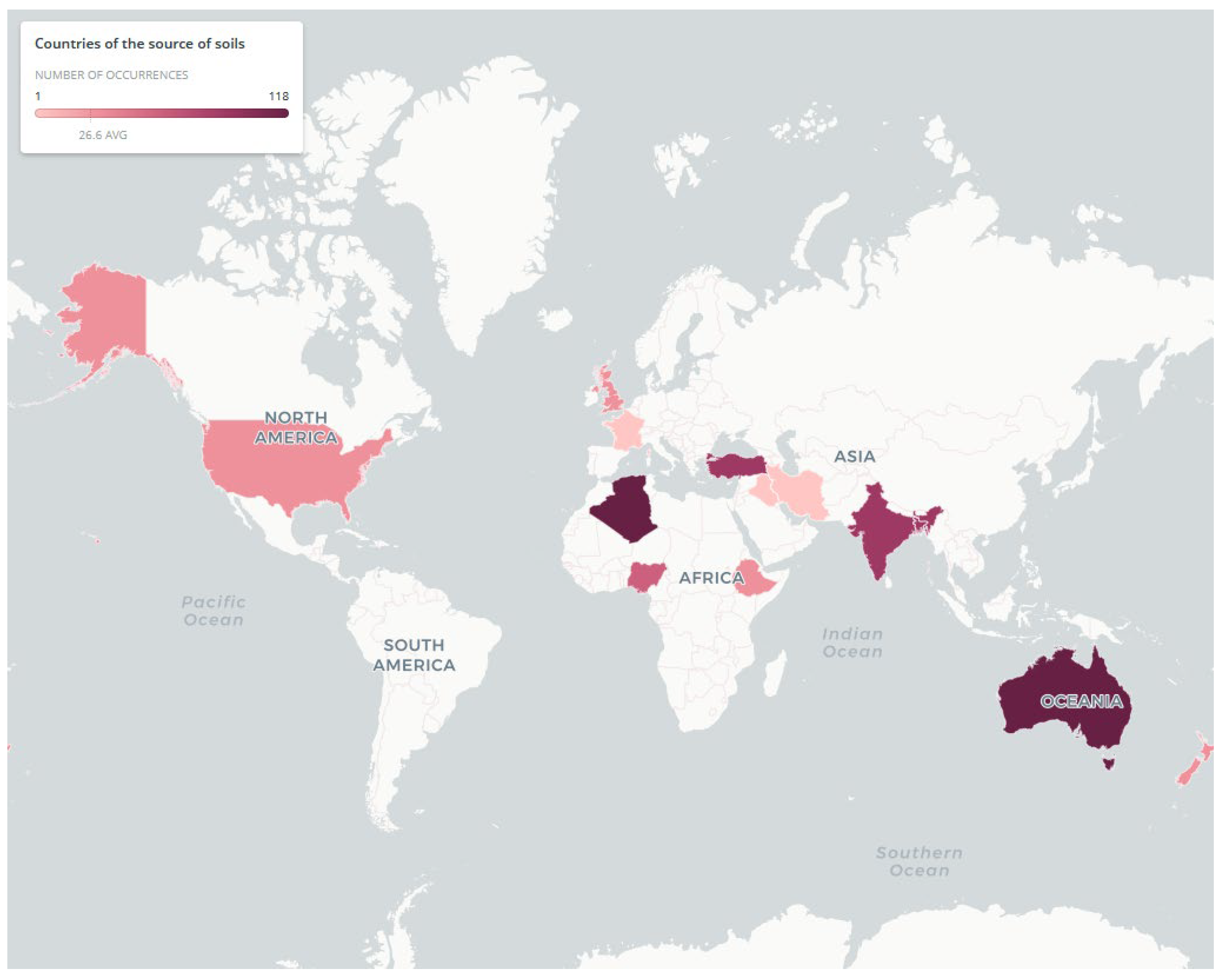
2.1. Experimental Data

Experimental data of stabilized as well as natural soils were obtained from the published literature to build a database for the construction of OMC, MDD, and UCS prediction models. Peer-reviewed literature accessed from Web of Science and Scopus databases were mainly utilized. Data comprised of 408 instances and 13 features containing information on the proportion of stabilizers (pozzolans, cement, lime, fly ash, and hydrated lime) and soils, values of Atterberg limits (liquid limit (LL), plastic limit (PL), and plasticity index (PI)) and compaction properties (OMC and MDD), classification of types of soils, and UCS of soils at various ages were gathered. The data set includes a variety of soils from 12 nations in Africa, Asia, Europe, North America, and Oceania. Figure 1 presents the distribution of the experiments in each continent/country wise. Countries represented by a dark red color contributed a large number of experimental data, whereas countries designated by a light pink color consist of few numbers of the cases. Among all countries, the highest number of experiments considered in this study are those obtained from Australia, which are 118 cases.

2.2. Machine Learning

In this work, two types of machine learning algorithms are adopted. These are the optimizable ensemble method and the artificial neural networks. In fact, examining other types of machine learning algorithms are also crucial since the relative predictive power of any algorithm is primarily determined by the specifics of the problems under consideration. It is impossible to identify the powerful algorithms that could excel for a given problem without experimentation. As the primary goal of this work is to investigate the applicability of machine learning on a variety of stabilized soils, the OEM was chosen because it typically produces more accurate results than a single model. The ANN algorithms are used for comparison with the OEM as the ANN are the most commonly used for such cases.
The application of machine learning algorithms, including those adopted, in the field of civil engineering is not novel. These domains have many practical applications, for instance [13,14,15,16,17,18,19,20,21]. The following subsections provide basic principles of the optimizable ensemble methods and the artificial neural networks.

2.2.1. Optimizable Ensemble Method

The basic premise of any ensemble technique is to create a powerful predictive model by combining numerous base models that individually address the same problem [22]. Although there are other ensemble methods in literature, bagging and boosting regression trees are the two examples of ensemble models. These techniques have been shown to be effective in tackling difficult regression problems for a wide range of datasets [23,24].

Bagging Regression Tree

The base models in a bagging regression tree are constructed using numerous randomly selected bootstrapped samples from the original dataset. This process is repeated until a significant portion of the training datasets have been created and the same samples can be collected multiple times. Each created bootstrapped training dataset contains on average N ( 1 1 e )   0.63 N observations, where N is the number of instances in the original dataset. Instances which are left out are called out-of-bag observations and are used to evaluate the performance of the models.
The final output of the bagging regression tree model is the average of the expected outputs of the multiple base models, reducing variance and improving stability [22,25]. The model of a bagging regression tree fits the training dataset D = { ( x 1 , y 1 ) , ( x 2 , y 2 ) , , ( x N , y N ) } , resulting in the tree’s prediction f ^ ( x )   for an input vector x . The base models generate prediction f ^ * t ( x )   for each bootstrap sample D * t ,   t = 1 , 2 , ,   T . Bagging averages this prediction over a set of bootstrap samples, as expressed by Equation (1).
f ^ b a g ( x ) = 1 T t = 1 T f ^ * t ( x ) .

Boosting Regression Tree

Boosting is a type of bagging that utilizes a large number of base models and focuses on scenarios that are difficult to perform successfully [23,25]. Boosting regression trees, in contrast to bagging, serially generate basic tree models that improve from one to the next and then merge them to enhance the model’s performance. It starts from a null model with r i = y i residuals for all i in the training dataset D = { ( x i , y i ) , i = 1 ,   , N } , where y . Then, instead of the outcome y, it fits a decision tree to the residuals of the model. The algorithm updates the residuals in a sequential manner by including the freshly formed decision tree in the fitted function. By adjusting the algorithm’s parameter d (number of splits), each of these trees can be made smaller to some extent. In regions where performance is poor, the   f ^   is gradually improved by fitting small trees to the residuals. The learning process is further slowed down by the shrinkage parameter, λ (learning rate). The number of iterations required to achieve a given training error raises for a small value of λ . Equation (2) presents the output of the boosted model.
f ^ L S b o o s t ( x ) = f ^ ( x ) = t = 1 t λ f ^ t ( x ) .

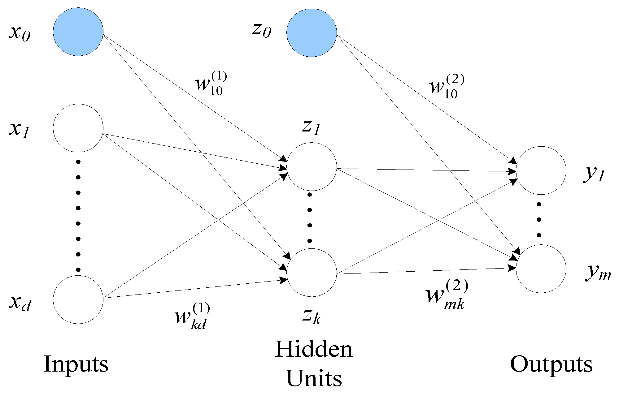
2.2.2. Artificial Neural Networks

Artificial neural networks are computational networks that are based on biological neural networks and consist of partially or fully coupled basic processing units known as artificial neurons. Each neuron analyses inputs on a local level, similar to how the brain learns [26]. Because the connections inside the network may be systematically modified based on inputs and outputs, ANNs is perfect for supervised learning. The multilayer feedforward architecture, in combination with the backpropagation training technique, is widely used to tackle difficult nonlinear regression problems [27,28], which is used in this study. A multilayer feedforward neural network with a single hidden layer is shown in Figure 2. The input and output layers are the first and last layers, respectively. A hidden layer is an intermediate layer that helps to do the necessary computations before passing the input data to the output layer. This network can be thought of as a nonlinear parametric function that connects a set of   x i   inputs to a set of y m outputs. The weighted inputs are first combined into linear combinations. This includes the network’s additional external inputs, known as bias, which are illustrated by the blue neurons in Figure 2. Biases have little effect on the network’s performance, but they do boost the network’s flexibility in adapting to the inputs. After linear combinations, an activation function (.), as shown in Equation (3), is used to transform them to new values [26,28]. The outputs of the first-hidden layer neurons are then multiplied by the layer’s interconnection weights that connect them to neurons in the next layer, as shown in Equation (4). If there are numerous hidden neurons in the network, this activity will continue until the output neurons compute the output values.
z j = φ ( i w j i ( 1 ) x i ) ,
y m = j w m j ( 2 ) z j ,
where w j i ( 1 ) and w m j ( 2 ) are the network’s weights, which are first set to random values and then adjusted as the network is being trained using the backpropagation process.

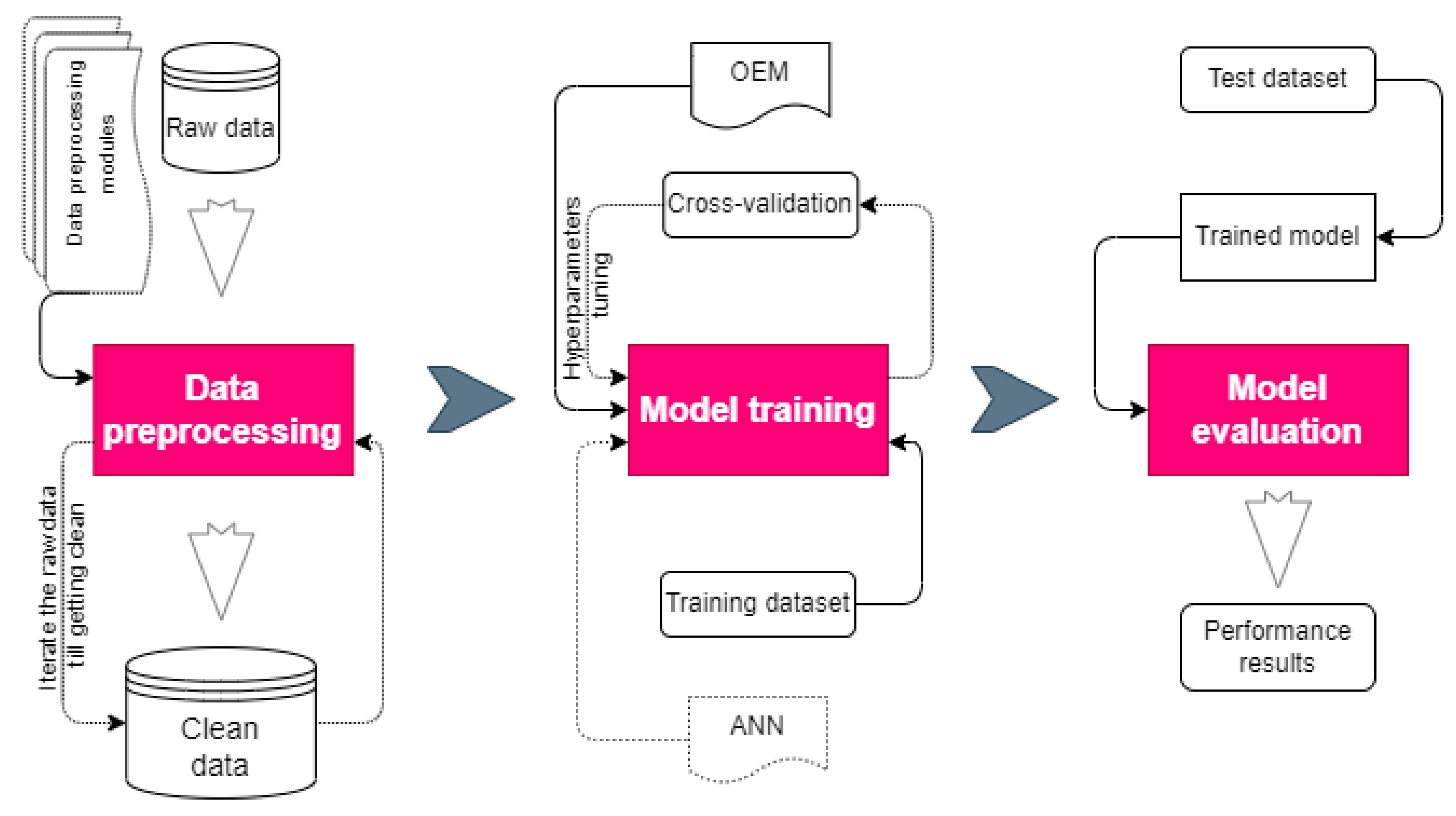
2.3. Model Development

The model development process for predicting OMC, MDD, and UCS is presented in this section. The primary task of the process is to retrieve the collected experimental data containing information on the mixing ratio of natural soils and stabilizers, soil classification, Atterberg limits, curing ages, physical and mechanical properties of the stabilized soils. After retrieving data, the preprocessing of the data follows. Under data processing, several activities are carried out, including outlier detecting and treating, data encoding, data normalization, feature engineering, and data partitioning. The next most important step is model training (fitting the data using machine learning algorithms of optimizable ensemble methods and ANN). The process of model training will be iterated until the best cross-validation results are obtained by optimizing the hyperparameters. The models’ performance is then assessed using a test dataset that is previously unseen by the model. Figure 3 shows the pipeline of the prediction models OMC, MDD, and UCS.

2.3.1. Data Preprocessing

Data preprocessing is one of the most important phases in any machine learning-based model development process. Before performing the vital data preprocessing tasks, the distribution of each feature was analyzed. Features for which there are insufficient representative instances were omitted from the dataset. These are pozzolans, fly ash, hydrated lime, and curing age. The collected data also includes unconfined compressive strength tests conducted at different ages. With the exception of UCS at 28 days of age, other age groups account for 1% to 15% of the total dataset. As a result, only unconfined compressive strength tests conducted at the age of 28 days are counted. The description of the selected features is disclosed in Table 1. The required data preprocessing activities carried out in this work are presented in the following subsections.

2.3.2. Detecting and Treating Outliers

Outlier detection is an important activity in any data-driven model development process as the model performance is dependent on the quality of the data. Outliers are relatively extreme observations that are very dissimilar to the rest of the population. A box plot is one of the methods used to identify outliers from numeric features through their interquartile range (IQR). Figure 4 is the box plot of the features that represents the Atterberg limits (LL, PL, and PI). A box plot describing the physical and mechanical properties of the natural and stabilized soils (OMC, MDD, and UCS) is revealed in Figure 5. In the box plots, the median of the considered attributes is represented by a line within the box that encompasses the middle 50% (25–75th percentiles) of their values. The whiskers go all the way down to the smallest and all the way up to the greatest feature values. Outliers are defined as values that are more than 1.5 box lengths above the whiskers and are denoted by a diamond sign. It can be noticed from Figure 4 and Figure 5 that all features, except MDD, comprise outliers (value 1.5 IQRs greater than the third quartile). All the outliers are dropped from the dataset.

2.3.3. Data Encoding

Not all machine learning algorithms can handle a variety of data types (continuous and nominal). OEM, for example, can handle both continuous and nominal data types without issue, but ANN cannot handle nominal data types. Because ANN is used in this study, all non-numeric variables must be encoded as numerical variables. To do this, the ordinal encoding technique was applied. It is one of the common approaches that assigned each unique category value with an integer value.

2.3.4. Data Normalization

Normalizing input and target features before feeding them to artificial neural networks is a standard practice. It aligns the features on a similar scale, which is critical if they are on different scales. The formula described in Equation (5) is used to normalize all of the input and target features.
y = ( y m a x y m i n ) ( x x m i n ) ( x m a x x m i n ) + y m i n ,
where; y is the feature’s normalized value; y m a x is the maximum value of the normalization range, (+1); y m i n is the minimum value of the normalization range, (−1); x is the original input or target features; x m a x is the maximum value for feature   x ; and x m i n is the minimum value for feature   x . If x m a x = x m i n or if either x m a x or x m i n is non-finite, y = x and no change occurs. After normalization, the values of the input and target values fall into the range [−1, 1].

2.3.5. Feature Engineering

Feature engineering is also a critical component of the data preprocessing phase of the machine learning model construction process, as it has a significant impact on the model’s performance. A machine learning algorithm cannot predict data for which it does not have any prior information. Feature engineering is usually conducted by experts who have the appropriate domain knowledge, and the majority of the essential feature engineering tasks were already completed during the compilation of information from previously released publications. For instance, some studies use different measuring units or soil classification methods. All data were translated into the appropriate unit and format.
Descriptive statistics of the numeric features of the preprocessed data which are going to be used to train the model are illustrated in Table 2. It can be noticed that the finally selected data comprise 162 observations. The stabilized soils included in this database had unconfined compressive strengths ranging from 55.31 to 4900 kN/m2, all tested at their 28th days. The values of OMC and MDD range from 5.40–28.00% and 1440–2210 kg/m3, respectively.
Cement and/or lime are used to stabilize all soils. Despite the fact that there are several cement and lime types, they are not specifically indicated in the literature from which the data were taken. The dataset employs five different types of soil (which are classified in accordance with Unified Soil Classification System (USCS)), and their proportion is depicted in Figure 6a. These are low plasticity clay (CL), high plasticity clay (CH), silt (ML), high plasticity silt (MH), and clayey silt (CL-ML). CL and ML soil types account for 58.6% and 25.9% of the total, respectively. CH, CL-ML, and MH account for the remaining 15.5%. The proportion of the utilized stabilizers in the dataset is presented in Figure 6b. Soils stabilized by cement have the greatest portion of 42%, followed by cement and lime of 32.1% and lime of 21.6% stabilizers.

2.3.6. Data Partitioning

Typically, data is divided into training and test sets. The training set is used to train the model, while the test set is used to assess the fitted or built model’s prediction performance on data it has never seen before. In the case of the optimizable ensemble approach, the data were divided into two parts: 80% for training and 20% for testing. The K-fold cross-validation procedure was used because the data were limited. With this method, the training dataset is randomly divided into K subgroups of almost equal size. A validation dataset is used for each K subset to examine the performance of the model, while the training dataset is used for the remaining (K − 1) subsets. A total of K models are fitted, and K validation statistics are acquired. The K-fold performance ratings are then averaged to determine the model’s overall performance. In this work, a 10-fold cross-validation technique was used. The data for ANN was split into three subsets: training, validation, and test. The training dataset was used to compute the gradient and adjust the network’s weights and biases. The validation dataset is applied to stop the model training when the generalization process stops increasing. Of the total data, 70% was the training dataset, 15% was the validation dataset, and 15% was the testing dataset.

2.4. Model Training

2.4.1. Optimizable Ensemble Methods

Regression trees are fitted using bootstrap samples and then aggregated for the purpose of building bagged regression trees. In addition, boosting regression trees are created as a result of iteratively fitting multiple regression trees when the model training at each step is determined by the previously fitted model. Each new model concentrates on the most difficult situations, resulting in a strong learner. Three models for predicting OMC, MDD, and UCS of natural and stabilized soils are built using the optimizable ensemble method. This means that both methods, bagging and boosting, will be tested and the one that gives the best results will be chosen as the final model. All seven features listed in Table 1 under the categories soil and stabilizers, soil classification, and Atterberg limits are used to predict OMC and MDD of soils. Two extra features (nine in total) were used in the UCS prediction model. Indeed, all the features may not be utilized as a predictor since the employed optimizable ensemble method can select the most significant features.
To improve the performance of any machine learning-based model, the hyperparameters must be fine-tuned. In this study, in conjunction with a 10-fold cross-validation, hyperparameter fine-tuning is conducted using Bayesian optimization, which determines the ideal combination of values of hyperparameters that minimizes the mean-square error (loss function). The following hyperparameters are considered, along with their search ranges: (i) Ensemble method—Bag and LSBoost; (ii) Number of learners—integers log-scaled in the range [10, 500]; (iii) Learning rate—real values log-scaled in the range [0.001, 1]; (iv) Minimum leaf size—integers log-scaled in the range [1, max (2, floor (n/2))], where n is the number of observations; and (v) Number of predictors to sample—integers in the range [1, max (2, p)], where p is the number of predictor variables.

2.4.2. Artificial Neural Networks

Three ANN-based models are also developed to predict the OMC, MDD, and UCS of natural and stabilized soils. The basic architecture of the developed ANN models is the same as the one illustrated in Figure 2. Each of the models has three fully connected layers: an input, a hidden, and an output layer. The network input features (predictors) connect the first fully connected layer of the ANN, and each successive layer connects to the preceding layer. Each fully connected layer adds a bias vector after multiplying the input by a weight matrix and then an activation function follows. The hyperbolic tangent transfer function was chosen as the activation function for each model’s hidden layers. This function provides outputs ranging from −1 to 1 as the neuron’s input changes from negative to positive infinity. The output layer of the network was given a linear transfer activation function for each model. It conveys the neuron’s output by passing the value supplied to it. The input layer does not have an activation function since it has to convey inputs to the hidden layer. The final fully connected layer of the developed three models produces the network’s output, which are the predicted response values of OMC, MDD, and UCS.
In this work, the inputs and targets of the OMC, MDD, and UCS datasets are mapped using three backpropagation algorithms: Levenberg–Marquardt, Bayesian Regularization, and Scaled Conjugate Gradient. Levenberg–Marquardt calculates each neuron’s error contribution after a batch of training data is processed [30]. To modify the weight of each neuron, the error computed at the output is transmitted back through the network layers. The Bayesian Regularization approach also uses Levenberg–Marquardt optimization to update the weight and bias values, although it can result in good generalization for small datasets at the cost of time [31]. Scaled Conjugate Gradient modifies weight and bias values in accordance with the scaled conjugate gradient method [32]. This approach searches in conjugate directions, which usually results in a faster convergence time. The optimal number of neurons in the hidden layer was also established based on the generalization error after running numerous trainings with three, five, and ten neurons.

2.5. Model Evaluation

After finding the best hyperparameters for each model, the performance is assessed by evaluating the mean-square error (MSE) and coefficient of determination ( R 2 ). The MSE is calculated by averaging the squared difference between the actual and predicted values. Both MSE and R 2 are widely used for evaluating the performance of the regression models. The difference between MSE and R 2 is that MSE gets pronounced based on the value of the data. Instead of the MSE, which records the residual error, R 2 , represents the fraction of variance of the response feature obtained by the regression model. Due to enhanced interpretability of the model’s performance, R 2 is also known as the standardized version of MSE. The formula for calculating MSE is shown in Equation (6) below. The value of R 2 can be calculated using the formula given in Equation (7). If R 2 = 1 , the model fits the data perfectly, yielding an MSE of 0.
M S E = 1 n i = 1 n ( y i y ^ i ) 2 ,
R 2 = 1 1 n i = 1 n ( y i y ^ i ) 2 1 n i = 1 n ( y i y ¯ ) 2 = 1 M S E V a r   ( y ) ,
where n is the number of instances,   y i   is the value of the actual target feature, y ^ i is the value of the predicted output feature, y ¯ is the mean of the actual target feature, and V a r is the variance of the target feature.

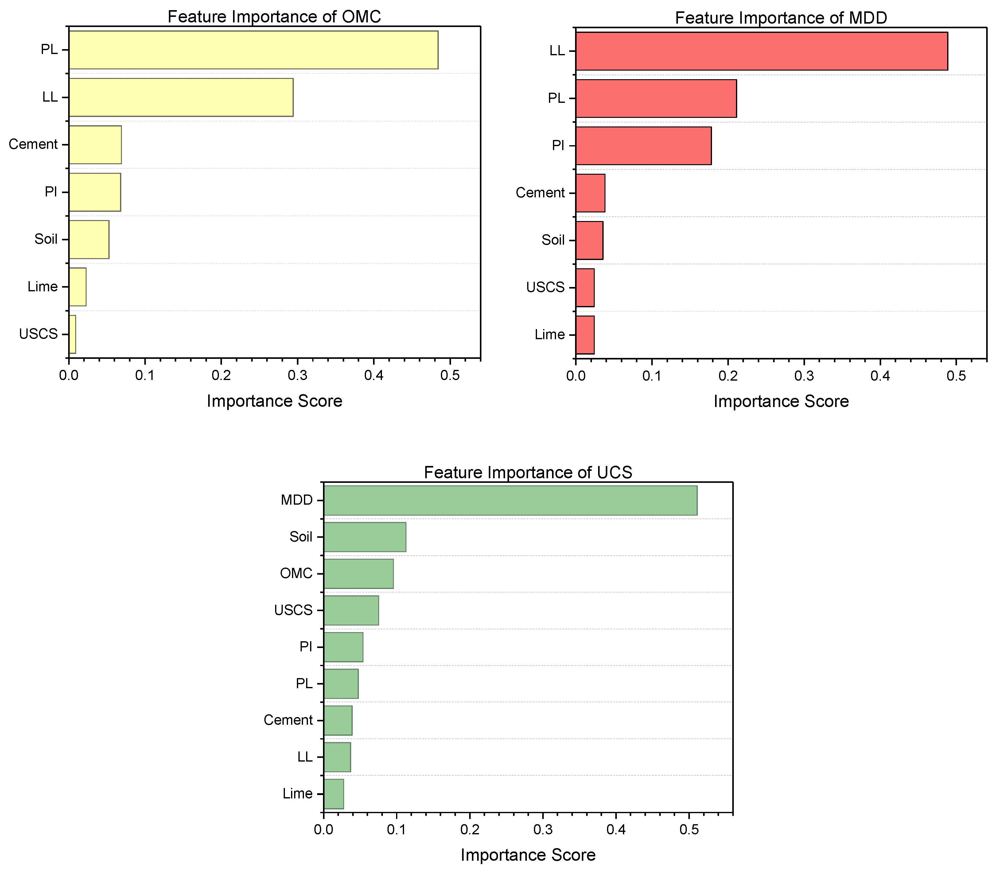
3. Results and Discussion

The performances of all the developed OMC, MDD, and UCS models are reported in this section. The training and test performance of all the models are presented in Table 3. The MSE is applied to measure the performance of the models. The lower the MSEs, the better the performance of the model. Indeed, the MSE comparison shall be done between models that predict the same features as the errors are computed using the actual values (not scaled) which are considerably varied. For example, the value of MDD and UCS is four digits whereas OMC is two digits, so it is obvious that the MSE of MDD and UCS will be much higher compared to OMC. As with any machine learning model, the validity of the created models should be validated using a test dataset that is obtained from the source data but differs from the training dataset. The goal is to see how well the model performs in real conditions.
Table 3 shows that the MSE of OEM-based OMC, MDD, and UCS models in the test dataset are 12.77, 34,410, and 370,860, respectively, while the corresponding models based on ANN are 8.84, 33,958, and 457,271. It can be noticed from the statistical errors that the performances of OEM and ANN-based MDD prediction models are quite comparable. The MSE of an ANN-based OMC prediction model is lower than the OEM version. However, in the case of UCS, the MSE of an OEM-based model is lower than the ANN one. Another statistical measure used to evaluate the effectiveness of all the models is the coefficient of determination, or R 2 . The R 2 value demonstrates how effective the developed OMC, MDD, and UCS models are in predicting and explaining the outcomes. It returns a score ranging from 0 to 1. Table 3 shows that the OMC and UCS models have a higher R 2 score than 0.50. Evidently, UCS models perform best ( O E M R 2 = 0.61 and A N N R 2 = 0.65), followed by OMC ( O E M R 2 = 0.56 and A N N R 2 = 0.65). Of all the models, the MDD models perform the least with ( O E M R 2 = 0.21 and A N N R 2 = 0.25). The cause for this could be the treatment of the outliers observed in the other features. As discussed in model development section, MDD was the only feature that did not comprise outliers. However, the drop of the outliers observed in the other features reduces the number of representative instances. Figure 7 reveals the distribution of MDD before and after outliers from other features were dropped. It can be seen from Figure 7 that the IQR (showing the middle 50% of scores) and the minimum 25% of the MDD after the outliers of the other features treated were dropped. It seems the reduction of the number of representative observations causes the MDD models to perform weakly. This corroborates that the inclusion of more and more data is essential to enhance the performance of the machine learning-based models, and it could eventually replace the time-consuming and expensive laboratory examination on both natural and stabilized soils.
Evaluation of the model’s performance using the aforementioned statistical metrics validates that the adopted algorithms predict compaction and strength properties of the soil with relatively low error on new data. In fact, these results are solely valid for the dataset that was used. If alternative data were used, the performance of each algorithm might differ. It is also worth noting that neither OEM nor ANN provide superior results in all models during training and test. There are cases where OEM provides better results than ANN, and vice versa. Assessing the performance of multiple machine learning algorithms for the prediction of OMC, MDD, and UCS is imperative to distinguish which algorithm performs best. This is because every machine learning algorithm’s relative prediction capacity is largely determined by the data and characteristics of the problems under consideration. It is impossible to distinguish the algorithms that excel at a given problem without experimenting with them.
Table 4 depicts the optimized hyperparameters of the OEM and ANN models. To optimize the performance of the OEM-based models, five hyperparameters were considered, as presented in the model training section. Hyperparameter tuning was performed using Bayesian optimization in combination with a 10-fold cross-validation technique to determine the ideal combination of values of hyperparameters that minimizes the mean-square error. Bagged regression trees produced the best results for OMC and MDD models. LSBoost provides a better result for UCS prediction with a minimum leaf size of 2 and a learning rate of 0.157. The number of predictors to sample and learners for each model is different.
In the case of ANN models, the Bayesian Regularization backpropagation algorithm provides optimal results for all models among the choices. The optimal number of neurons in the hidden layer was 5 for OMC and 10 for each MDD and UCS prediction models.
The adopted ensemble methods measured the relative importance of each feature in predicting OMC, MDD, and UCS, as shown in Figure 8. The feature importance score added up to one. It can be observed that the Atterberg limits (especially LL and PL) are the most influential predictors of OMC and MDD. These two features (LL and PL) do account for 78% and 70% of the predictive power of the OMC and MDD models, respectively. In the case of the UCS model, MDD is the most influential predictor than any feature. This feature alone accounted for 51% of the model’s predictive power, followed by soil (11%), and OMC (10%). Although Atterberg limits are very important features, they are not considered as potential predictors of UCS. This is because the MDD and OMC features already have their information encoded.
In the effort pursued to refine the earlier attempts on the topic considered to ascertain confidence through different approaches and methods, there is a need for further streamlining to attain a point of proven satisfaction. The reason behind this is the complexity of nature’s innateness, be it in depth and breadth or otherwise. The addition of amending material to the already yet non-graspable natural soil intricacy is just like destabilizing a system which is in a state of equilibrium exponentially. In this regard, the outcome of any scientific endeavor might end in moderating or exacerbating the problem at hand. This in turn invites a change of direction or to a more surgical approach to break the impasse. Thus, the search continues.

4. Conclusions

In this work, OMC, MDD, and UCS prediction models were developed by adopting an optimizable ensemble method and artificial neural networks. To build a database for model development, experimental data were collected from a variety of natural and stabilized soils from previously published studies. Seven features were used in the OMC and MDD models, describing the proportion of the soil and stabilizers, soil classification, and Atterberg limits. The USC prediction models use all the seven features used in the OMC and MDD prediction models, plus the OMC and MDD features, for a total of nine input features. All generated models performed well and demonstrated their ability to make predictions with low error. Neither OEM nor ANN provide superior results in all cases. There are instances where OEM provides better results than ANN, and vice versa. To that effect, possible scientific reasons for the anomalies are noted to be the starting points for future studies. Indeed, in the future, exploration of several machine learning algorithms is imperative to identify the one that predicts the OMC, MDD, and UCS in the best possible way. With more data, the performance of the models could be improved even further, and they could be used to calculate the optimal stabilizers ratio that results in the desired OMC, MDD, and UCS values. Consequently, the models can replace the laboratory examination of natural and stabilized soils, especially for developing countries, thus enabling the reduction of both time and resource consumption as well as cost. It could also lay a reliable foundation to draft earth-based construction material unifying standards to popularize mass housing projects the world over.

Supplementary Materials

The following supporting information can be downloaded at: https://www.mdpi.com/article/10.3390/buildings12050613/s1, Table S1: The dataset used to develop the OMC, MDD, and UCS prediction models.

Author Contributions

Conceptualization, W.Z.T. and K.A.A.; methodology, W.Z.T.; software, W.Z.T.; validation, W.Z.T.; formal analysis, W.Z.T.; investigation, W.Z.T. and K.A.A.; resources, W.Z.T. and K.A.A.; data curation, W.Z.T. and K.A.A.; writing—original draft preparation, W.Z.T. and K.A.A.; writing—review and editing, W.Z.T. and K.A.A.; visualization, W.Z.T.; project administration, K.A.A. All authors have read and agreed to the published version of the manuscript.

Funding

This research received no external funding.

Institutional Review Board Statement

Not applicable.

Informed Consent Statement

Not applicable.

Data Availability Statement

The data presented in this study are available in Supplementary Material here.

Conflicts of Interest

The authors declare no conflict of interest.

References

  1. Admassu, K. Hydration and carbonation reaction competition and the effect on the strength of under shed air dried amended compressed earth blocks (ACEBs). Zede J. 2021, 39, 19–29. [Google Scholar]
  2. Bahmed, I.T.; Harichane, K.; Ghrici, M.; Boukhatem, B.; Rebouh, R.; Gadouri, H. Prediction of geotechnical properties of clayey soils stabilised with lime using artificial neural networks (ANNs). Int. J. Geotech. Eng. 2019, 13, 191–203. [Google Scholar] [CrossRef]
  3. Alavi, A.H.; Gandomi, A.H.; Gandomi, M.; Sadat Hosseini, S.S. Prediction of maximum dry density and optimum moisture content of stabilised soil using RBF neural networks. IES J. Part A Civ. Struct. Eng. 2009, 2, 98–106. [Google Scholar] [CrossRef]
  4. Admassu, K. Engineered soil and the need for lime-natural pozzolan mixture percentage approximation. SINET Ethiop. J. Sci. 2018, 41, 70–79. [Google Scholar]
  5. Admassu, K. Method of amended soils for compressed block and mortar in earthen construction. Zede J. 2019, 37, 69–84. [Google Scholar]
  6. Alavi, A.H.; Gandomi, A.H.; Mollahassani, A.; Heshmati, A.A.; Rashed, A. Modeling of maximum dry density and optimum moisture content of stabilized soil using artificial neural networks. J. Plant Nutr. Soil Sci. 2010, 173, 368–379. [Google Scholar] [CrossRef]
  7. Das, S.K.; Samui, P.; Sabat, A.K. Application of Artificial Intelligence to Maximum Dry Density and Unconfined Compressive Strength of Cement Stabilized Soil. Geotech. Geol. Eng. 2011, 29, 329–342. [Google Scholar] [CrossRef]
  8. Saadat, M.; Bayat, M. Prediction of the unconfined compressive strength of stabilised soil by Adaptive Neuro Fuzzy Inference System (ANFIS) and Non-Linear Regression (NLR). Geomech. Geoengin. 2022, 17, 80–91. [Google Scholar] [CrossRef]
  9. Kalkan, E.; Akbulut, S.; Tortum, A.; Celik, S. Prediction of the unconfined compressive strength of compacted granular soils by using inference systems. Environ. Geol. 2009, 58, 1429–1440. [Google Scholar] [CrossRef]
  10. Suman, S.; Mahamaya, M.; Das, S.K. Prediction of Maximum Dry Density and Unconfined Compressive Strength of Cement Stabilised Soil Using Artificial Intelligence Techniques. Int. J. Geosynth. Gr. Eng. 2016, 2, 11. [Google Scholar] [CrossRef] [Green Version]
  11. Chore, H.S.; Magar, R.B. Prediction of unconfined compressive and brazilian tensile strength of fiber reinforced cement stabilized fly ash mixes using multiple linear regression and artificial neural network. Adv. Comput. Des. 2017, 2, 225–240. [Google Scholar] [CrossRef]
  12. Le, H.A.; Nguyen, T.A.; Nguyen, D.D.; Prakash, I. Prediction of soil unconfined compressive strength using artificial neural network model. Vietnam J. Earth Sci. 2020, 42, 255–264. [Google Scholar] [CrossRef]
  13. Fu, B.; Feng, D.-C. A machine learning-based time-dependent shear strength model for corroded reinforced concrete beams. J. Build. Eng. 2021, 36, 102118. [Google Scholar] [CrossRef]
  14. Fu, B.; Chen, S.-Z.; Liu, X.-R.; Feng, D.-C. A probabilistic bond strength model for corroded reinforced concrete based on weighted averaging of non-fine-tuned machine learning models. Constr. Build. Mater. 2022, 318, 125767. [Google Scholar] [CrossRef]
  15. Taffese, W.Z. Case-based reasoning and neural networks for real estate valuation. In Proceedings of the IASTED International Conference on Artificial Intelligence and Applications, AIA, Innsbruck, Austria, 12–14 February 2007; Devedzic, V., Ed.; ACTA Press: Innsbruck, Austria, 2007; pp. 84–89. [Google Scholar]
  16. Taffese, W.Z.; Sistonen, E.; Puttonen, J. Prediction of concrete carbonation depth using decision trees. In Proceedings of the 23rd European Symposium on Artificial Neural Networks, Computational Intelligence and Machine Learning, Bruges, Belgium, 22–23 April 2015; i6doc.com Publisher: Louvain-la-Neuve, Belgium, 2015. [Google Scholar]
  17. Kardani, N.; Zhou, A.; Nazem, M.; Shen, S.L. Improved prediction of slope stability using a hybrid stacking ensemble method based on finite element analysis and field data. J. Rock Mech. Geotech. Eng. 2021, 13, 188–201. [Google Scholar] [CrossRef]
  18. Ren, Q.; Ding, L.; Dai, X.; Jiang, Z.; De Schutter, G. Prediction of Compressive Strength of Concrete with Manufactured Sand by Ensemble Classification and Regression Tree Method. J. Mater. Civ. Eng. 2021, 33, 04021135. [Google Scholar] [CrossRef]
  19. Taffese, W.Z.; Sistonen, E. Significance of chloride penetration controlling parameters in concrete: Ensemble methods. Constr. Build. Mater. 2017, 139, 9–23. [Google Scholar] [CrossRef]
  20. Taffese, W.Z.; Nigussie, E.; Isoaho, J. Internet of things based durability monitoring and assessment of reinforced concrete structures. Procedia Comput. Sci. 2019, 155, 672–679. [Google Scholar] [CrossRef]
  21. Taffese, W.Z.; Abegaz, K.A. Artificial intelligence for prediction of physical and mechanical properties of stabilized soil for affordable housing. Appl. Sci. 2021, 11, 7503. [Google Scholar] [CrossRef]
  22. Alpaydin, E. Introduction to Machine Learning, 2nd ed.; MIT press: Cambridge, MA, USA, 2020; ISBN 978-0-262-01243-0. [Google Scholar]
  23. Cichosz, P. Data Mining Algorithms: Explained Using R; John Wiley & Sons, Ltd.: Hoboken, NJ, USA, 2015; ISBN 978-1-118-33258-0. [Google Scholar]
  24. Witten, I.H.; Frank, E.; Hall, M.A. Data mining: Practical Machine Learning Tools and Techniques; Morgan Kaufmann: Burlington, MA, USA, 2011; ISBN 978-0-12-374856-0. [Google Scholar]
  25. Berthold, M.R.; Borgelt, C.; Höppner, F.; Klawonn, F. Guide to Intelligent Data Analysis: How to Intelligently Make Sense of Real Data; Springer: London, UK, 2010; ISBN 978-1-84882-260-3. [Google Scholar]
  26. Haykin, S. Neural Networks and Learning Machines, 3rd ed.; Pearson Education, Inc.: Upper Saddle River, NJ, USA, 2009; ISBN 978-0-13-129376-2. [Google Scholar]
  27. Vinaykumar, K.; Ravi, V.; Mahil, C. Software cost estimation using soft computing approaches. In Handbook of Research on Machine Learning Applications and Trends: Algorithms, Methods, and Techniques; Olivas, E.S., Guerrero, J.D.M., Sober, M.M., Benedito, J.R.M., López, A.J.S., Eds.; IGI Global: Hershey, PA, USA, 2010; pp. 499–518. ISBN 978-160566-766-9. [Google Scholar]
  28. Wu, J.; Coggeshall, S. Foundations of Predictive Analytics; CRC Press: Boca Raton, FL, USA, 2012; ISBN 978-1-4398-6946-8. [Google Scholar]
  29. Taffese, W.Z. Data-Driven Method for Enhanced Corrosion Assessment of Reinforced Concrete Structures; University of Turku: Turku, Finland, 2020. [Google Scholar]
  30. Nguyen, G.H.; Bouzerdoum, A.; Phung, S.L. Efficient supervised learning with reduced training exemplars. In Proceedings of the IEEE International Joint Conference on Neural Networks, IJCNN 2008, Hong Kong, China, 1–8 June 2008; pp. 2981–2987. [Google Scholar]
  31. Al Bataineh, A.; Kaur, D. A Comparative Study of Different Curve Fitting Algorithms in Artificial Neural Network using Housing Dataset. In Proceedings of the IEEE National Aerospace Electronics Conference, NAECON, Dayton, OH, USA, 23–26 July 2018; pp. 174–178. [Google Scholar]
  32. Babani, L.; Jadhav, S.; Chaudhari, B. Scaled conjugate gradient based adaptive ANN control for SVM-DTC induction motor drive. In IFIP Advances in Information and Communication Technology; Iliadis, L., Maglogiannis, I., Eds.; Springer: Cham, Switzerland, 2016; pp. 384–395. [Google Scholar] [CrossRef] [Green Version]
Figure 1. Distribution of experimental data in multiple locations globally.
Buildings 12 00613 g001
Figure 2. A multilayer feedforward neural network with a single hidden layer [29].
Buildings 12 00613 g002
Figure 3. The pipeline of the prediction models OMC, MDD, and UCS.
Buildings 12 00613 g003
Figure 4. Box plot of LL, PL, and PI.
Buildings 12 00613 g004
Figure 5. Box plots of (a) OMC, (b) MDD, and (c) UCS.
Buildings 12 00613 g005
Figure 6. The proportion of soil types and stabilizers in the dataset. (a) soil types, (b) soil plus stabilizers.
Buildings 12 00613 g006
Figure 7. Distribution of MDD before and after outliers from other features were dropped.
Buildings 12 00613 g007
Figure 8. The feature importance score of the OMC, MDD, and UCS predictive models.
Buildings 12 00613 g008
Table 1. Description of the features employed in the dataset.
Feature CategoryNo.Feature Subcategory
Soil and stabilizers1Soil
2Cement
3Lime
Soil classification4USCSCH
CL
CL-ML
MH
ML
Atterberg limits5Liquid limit
6Plastic limit
7Plasticity index
Physical and mechanical properties8Optimum moisture content
9Maximum dry density
10Unconfined comprehensive strength
Table 2. Descriptive statistics of the dataset.
SoilCementLimeLLPLPIOMCMDDUCS
count162162162162162162162162162
mean93.893.722.4034.3720.2014.1811.831835.882466.12
std3.443.283.5410.155.978.844.60182.941070.11
min70.000.000.0018.0012.000.005.401440.0055.31
25%94.000.000.0027.0016.006.108.551700.001860.00
50%94.004.002.0032.0019.0015.0010.501835.002300.00
75%95.006.004.0040.0023.0020.0013.381970.003075.00
max100.0030.0030.0066.0039.0042.0028.002210.004900.00
Table 3. Statistical performance evaluation of the developed OEM and ANN-based models.
AlgorithmLearning MethodTraining ErrorTest Error
MSE R 2 MSE R 2
OEMOMC9.690.4812.770.56
MDD22,0540.2734,4100.21
UCS295,9000.75370,8600.61
ANNOMC5.700.738.840.55
MDD25,6700.1933,9580.25
UCS241,7300.79457,2710.65
Table 4. Hyperparameters that yielded the optimal results.
Optimizable Ensemble MethodsArtificial Neural Networks
Ensemble MethodMinimum Leaf SizeNo. of LearnersLearning RateNo. of Predictors to SampleAlgorithmsNo. of Hidden Neurons
OMCBag1475-7Bayesian Regularization5
MDDBag1402-5Bayesian Regularization10
UCSLSBoost24930.157086Bayesian Regularization10
Publisher’s Note: MDPI stays neutral with regard to jurisdictional claims in published maps and institutional affiliations.

